DeepFinder: An integration of feature-based and deep learning approach for DNA motif discovery

ABSTRACT

We propose an improved solution to the three-stage DNA motif prediction approach. The three-stage approach uses only a subset of input sequences for initial motif prediction, and the initial motifs obtained are employed for site detection in the remaining input subset of non-overlaps. The currently available solution is not robust because motifs obtained from the initial subset are represented as a position weight matrices, which results in high false positives. Our approach, called DeepFinder, employs deep learning neural networks with features associated with binding sites to construct a motif model. Furthermore, multiple prediction tools are used in the initial motif prediction process to obtain a higher number of positive hits. Our features are engineered from the context of binding sites, which are assumed to be enriched with specificity information of sites recognized by transcription factor proteins. DeepFinder is evaluated using several performance metrics on ten chromatin immunoprecipitation (ChIP) datasets. The results show marked improvement of our solution in comparison with the existing solution. This indicates the effectiveness and potential of our proposed DeepFinder for large-scale motif analysis.

KEYWORDS:

• Deep learning neural network
• motif discovery
• DNA sequence feature
• chromatin immunoprecipiation-sequencing analysis

Introduction

The ability to identify transcription factor binding sites or motifs in the genome is one of the keys to decipher gene regulation mechanisms. Motifs are recurring sequence patterns in a genome and are the binding sites of transcription factors crucial for the regulation of protein production in cells. Analysis of motifs is important for advancements of medical treatment and understanding of cell processes [1]. Both wet-lab and computational techniques have been widely employed for location identification and analysis of motifs.

Motif analyses with chromatin immunoprecipitation (ChIP) combined with massive parallel DNA sequencing (ChIP-seq) followed by computational prediction have enabled rapid genome-wide location prediction of thousands of high-confidence candidate motif locations. Genome-wide datasets have posed several challenges to the computational algorithm design because of increasing complexities of the sequence search space and the requirement of a large amount of memory space. Early methods for genome-wide motif discovery are based on comparative genomic [2] and motif profile search. The comparative genomic method is based on the principle that functional elements (e.g. motifs) evolved from the common ancestors are conserved, compared to their surrounding non-functional bases. Therefore, such conserved functional elements can be identified by performing conservation analysis between sequences of orthologous or paralogous species using pair-wise and multiple sequence alignment techniques. GenomeVISTA [3], LAGAN/MLAGAN [4], MUMmer [5], AVID [6] and MULAN [7] are examples of such tools. They are mostly based on the dynamic programming algorithm such as Smith–Waterman [8] for the local alignment and Needleman–Wunsch [9] for the global alignment. To speed up the alignment of genomes, heuristic techniques such as anchoring [6], threaded blockset [10] or greedy search [11] have been employed. Although comparative genomic methods enabled identification of conserved motifs, these methods missed many functional motifs that are not conserved [12]. The second group of methods uses a database of annotated motif profiles to detect associated sites in input datasets [13–16]. Motifs are typically represented as a position weight matrix (PWM) [17] or its variants [18]. MATCH [13] combines the matrix and core similarity score for scoring a sequence; MISCORE [14] computes the average mismatch score between a sequence and motif instances for scoring; the MAST [19] score of a sequence is simply the sum of the PWM's entries that matched the nucleotides in different positions of the sequence; FIMO computes the log-likelihood ratio score for each sequence and converts it into p-value for scoring purposes. The disadvantages of the motif profile search method are: first, it cannot effectively represent the specificities of DNA segments recognized by transcription factors (TF); second, a single representation cannot model the different ‘codes’ recognized by different TFs. For instance, some motifs have dependencies while others do not [20]. As a result, most PWM models give poor sensitivity and specificity in motif detection.

The advantages of the approach involving computational prediction of motif patterns are its cost effectiveness and its ability to hypothesize candidate binding sites before wet-lab verification is performed. The ultimate aim of motif prediction tools is to return a set of most potential putative binding site locations. Pre-genomic era tools were targeted mainly on small datasets from prokaryotic species, which cannot be scaled in terms of accuracy and speed [21]. Popular tools in that era can be categorized into multiple local alignment (AlignACE [22], MEME [23], BioProspector [24], MotifSampler [25]), pattern enumeration (MDSCAN [26], Weeder [27]) and heuristic search (GAME [28,29]). With the invention of the ChIP technology, genome-wide motif analysis has become feasible with many computational tools being proposed. Most of these tools employed heuristics and pattern enumerative approach to search for possible motif patterns for their efficiency. That is, instead of enumerating exhaustively all motif patterns of specified lengths, a heuristic algorithm initially selects statistical significance seed consensus motif patterns which for examples are short (3–8 bp in DREME [30]) or short patterns spaced by gaps [31]. Seeds are used to form longer patterns or initialize a search algorithm. Computational time, thus, is significantly reduced by starting the search using the resulting sub-optimal motif patterns. Although these tools are useful, most can only predict short motif patterns. A genetic algorithm-based tool has also been proposed [32], but search-based tools are not scalable.

A recently published article made an intriguing finding regarding the theoretical limit of the number of DNA sequences that should be used for computational DNA motif discovery [33]. The authors reported that increasing the number of input sequences does improve the motif prediction accuracy; however, after it reaches a certain quantity, the improvement is no longer significant. This finding contradicted many studies that assumed that better results can be expected when more input sequences are used for computational tools. This implies that a sufficient number of input sequences will be adequate to predict motifs in a dataset, and it is not necessary to use the whole set as input for computational tools.

The finding by Zia and Moses [33] was evidenced in an earlier study by Hu et al. [21], who reported that using more input sequences does not improve the prediction accuracy. They suggested that ‘one can input only partial input sequences to a motif discovery algorithm to obtain a motif model and then use this model to find motifs in the remaining sequences. In this manner, a significant reduction in the running time can be achieved without sacrificing the prediction accuracy.’ The accuracy of that method holds when: (a) The primary motif's appearances in the dataset are evenly distributed in the dataset of a sufficiently large size. (b) The primary motif model obtained from the partial input sequences can effectively detect associated binding sites in the remaining sequences. To the best of our knowledge, this finding has not been incorporated into the design of any tool. In fact, many newly proposed computational motif prediction tools [34] are designed to tackle large numbers of DNA sequences. Examples of such tools are AMD [31], RSAT peakmotifs [34] and DREME [30], which are based on consensus pattern enumeration; genetic algorithm based GADEM [35], and CompleteMotifs [36], which employs multiple motif discovery tools. Some authors have employed an ad-hoc motif discovery pipeline that works per the recommendation by Hu et al. [21]. We termed this strategy the three-stage approach.

In this study, DeepFinder, a motif discovery pipeline, is proposed to improve the current implementation of the three-stage method. The two novel features of this approach are: first, we employ an ensemble of motif discovery tools for initial prediction of candidate binding sites from a subset of input sequences; second, features associated with the most potential candidate binding sites are extracted for deep neural network learning. Using ten ChIP datasets for evaluation, our results have demonstrated that DeepFinder is able to improve the overall sensitivity and specificity rates in comparison to the three-stage approach.

Related works

The three-stage approach tackles the motif search in a large ChIP dataset by dividing the task into three consecutive steps [37,38]: (1) select a small subset of input dataset; (2) perform motif discovery in the subset using a computational tool and select the most potential candidate motifs; (3) use the candidate motif models to detect binding sites in the input subset not used in stage 1. The three-stage approach reduced the computational time significantly by avoiding the motif search in the whole sequence space. It conjectures that prominent motifs can be obtained using any subset of the input sequences of a reasonable size. The existing approach employed a single motif tool in stage 2 to predict candidate motifs. The obtained motifs are typically modeled using the PWM which are subsequently used for site detection in stage 3. Nevertheless, the existing solution is not robust. First, motif detection in the third stage relies on a good binding model that can represent a protein's specificities. Although PWM usually fits the binding affinity and specificity of a TF well, it is incapable of capturing motifs with positional dependencies. Second, in motif detection, setting the threshold value of a match is often difficult to ensure the balance of high sensitivity and specificity [39].

Supervised learning based on deep learning neural networks for enhancer motif prediction has become popular recently. DeepBind [40] employed convolutional neural networks (CNN) to identify the DNA- or RNA-binding regions. DeepBind's binding model showed excellent performance with an average area under curve (AUC) of 0.85, when it was trained on in vitro and tested on in vivo motif datasets, which outperformed the state-of-the-art methods using several performance metrics. DanQ [41] is a hybrid of convolutional and recurrent deep neural networks for learning enhancer-associated histone marks. It was claimed to outperform DeepSEA, another CNN-based model, using ChIP-Seq datasets for evaluation. However, DeepSEA's performance is still considered unsatisfactory with its precision-recall AUC being under 70%.

Materials and methods

Framework

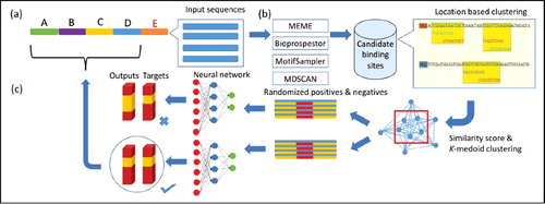
DeepFinder involves a three-stage approach that utilizes an ensemble of motif finders and machine-learning technique for motif prediction. Figure 1 illustrates the DeepFinder computational framework. It has three consecutive steps: (a) The dataset is partitioned into five non-overlapped subsets. (b) Four de novo motif discovery tools are applied on one of the partitioned subsets to predict putative motifs and the respective binding sites. The top three motifs returned from each tool are merged and divided using a clustering algorithm. Seventy-six features associated with candidate binding sites in merged clusters are extracted and used for stacked-autoencoder neural network learning. (c) Learned neural network is used to predict associated binding sites in input sequences not used in the initial motif prediction.

Figure 1. DeepFinder framework.

Candidate motif prediction and selection

A subset of input sequences is randomly selected from the input dataset motif prediction by four de-novo motif discovery tools: MEME [23], BioProspector [24], MDscan [26] and MotifSampler [25]. We employed toolbox of motif discovery (Tmod) [42], which implemented the four selected tools for candidate motif prediction. The top three motifs ranked by each tool's scoring function are selected for further processing. Putative site locations in the DNA sequences are located. Regions in DNA sequences where many overlapping putative sites are located are most likely to be legitimate binding regions. We called these regions binding segments (i.e. covered with at least one binding site or several overlapping binding sites in the vicinity). After identifying all binding segments, pairwise similarity between every possible pair is computed to generate a symmetry distance matrix (see the next subsection). Two clusters are generated by using the k-medoid clustering algorithm, implemented in Pycluster [43]. The cluster with a higher number of binding segments is fed as input to the deep learning neural network for building a binding model. We decided to generate two clusters because it is crucial to pursue more sequences in a cluster to avoid inadequate training data since there is no practical guideline on how many sequences are needed for model learning. Therefore, it is utterly important to keep the cluster number small in order to avoid missing any significant binding segments.

Motif similarity

We have modified the similarity function described by [44], to compute the similarity score of two binding segments x and y. Let A(x) = {x₁, x₂, …, x_n} be the set of binding sites clustered at binding segment x. The similarity score between two binding segments is computed from the average alignment of every pair of binding sites in the two segments. Suppose binding sites x_i ∈ A(x) and y_j ∈ A(y) have max(l(x_i),l(x_j)) – min(l(x_i), l(x_j)) + 1 possible alignment positions; l(x_i) is the length of x_i. Alignments of x_i and y_j are performed by starting at the left end position and then right shifting one base at a time, the shorter one on the longer ones. At a particular alignment position k, the alignment score is computed as $s_k \left(x_i,y_j\right)=\left|x_i\cap y_j\right|/\left|x_i\cup y_j\right|$, where |x_i ∩ y_j| is the number of matched nucleotides of the aligned two sites, |x_i ∪ y_j| is the total nucleotides in the alignment. Note that, 0  ≤ s_k(x_i, y_j) ≤ 1. Therefore, the similarity score between two binding sites x_i and y_j is defined as(1) $sim \left(x_i,y_j\right)=\sum _{1\le k\le m_{ij}}{s}_k\left(x_i,y_j\right) .$(1) The similarity score between two binding segments x and y is defined as(2) $sim \left(A\left(x\right),A\left(y\right)\right)= 1-\frac{{\sum }_{ij}sim(x_i,y_j)}{{\sum }_{ij}{m}_{ij}}.$(2) We use the scores obtained to populate our distance matrix, which is used by the k-medoid algorithm. As an illustrative example, suppose A(x) = {ATGCA, GCCG} and A(y) = {CGGA} are binding sites in each binding segment x and y, respectively. There are two pair-wise alignments between the two sets. The alignment pairs are (ATGCA, CGGA) and (GCCG, CGGA). The table below shows the alignment scores in different positions for the two pairs.

Table

		Position
x	y	1	2
ATGCA	CGGA	1/8	2/7
GCCG	CGGA	0

The following gives an example of how one of the alignment scores is obtained for the pair (ATGCA, CGGA). There is a total of max(l(ATGCA), l(CGGA)) – min(l(ATGCA), l(CGGA)) + 1 = 5−4 + 1 = 2 possible alignment positions as shown below.

Table

ATGCA	Score
CGGA-	1/8
-CGGA	2/7
Sum = 0.411

For alignment position 1, the score is 1/8 since there is a position (i.e. 3) where the nucleotide matched from the total nucleotides of 8. The matched nucleotide is counted as one for calculating |ATGCA ∪ CGGA−|. The alignment scores are summed to obtain 0.411 using Equation (1)(1) $sim \left(x_i,y_j\right)=\sum _{1\le k\le m_{ij}}{s}_k\left(x_i,y_j\right) .$(1) . The second pair is computed similarly which obtains sim(CGGA, GCCG) = 0. Finally, the similarity score between the two binding segments x and y is sim(A(x), A(y)) = 1− (0.411 + 0)/3 = 0.863.

Motif features

Several DNA sequence features are highly associated with binding sites. Osada et al. [20] reported that adjacent bases of motifs have high occurrence dependencies, which, when modeled, can significantly improve the motif prediction sensitivity and specificity rates. Furthermore, Yáñez-Cuna et al. [45] observed that enhancer regions have high occurrences of repeated dinucleotides CA, GA, CG or GC. For classifier learning, a feature vector comprising three distinct feature sets is generated from each DNA binding segment: (a) k-mer feature as a simple count of co-occurrences of bases that have strong dependencies, and k is set to 3, which gives 64 feature values; (b) the frequency counts of A, C, G, T; and (c) selected 2-mers count: CA, CG, GA and GC and the dinucleotide dependencies of CA, CG, GA and GC, where the dependency value of an arbitrary dinucleotide XY is computed as c(XY)/(c(XA) + c(XC) + c(XG) + c(XT)); c(⋅) is the frequency count in a binding segment. The feature value of a k-mer g is computed as f(g) = c(g)/c(*), where c(*) is the sum of counts from all possible k-mers. The frequency values are normalized using the min–max method.

Classifier learning

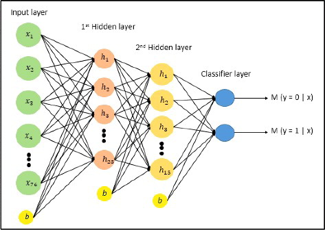
DeepFinder employs a stacked autoencoder [46] to construct binding models using the 76 engineered sequence features. The stacked autoencoder is well known for its feature discovery, especially in unlabeled data, and its capacity in part-whole decomposition. In addition, a single stacked autoencoder acquires greater expressive power compared with any deep learning neural network. An equal number of negative controls are added to the sequence segments of positive data to become the input dataset. The negative controls used are complementary intervals of the positive datasets retrieved from Galaxy Online [47]. The architecture of the stacked autoencoder used in this study is shown in Figure 2. It consists of two hidden layers, with 25 and 15 hidden neurons, respectively. The neural network was trained with a learning rate value between 0.5 to 1, mini-batch size of 100 and dropout value 0.5. We found that five fixed epochs were sufficient for the classifier to learn the features, since no significant improvement on the learning can be obtained when more epochs were used. Therefore, it is used for all the cross-validation experiments. The stacked autoencoder implemented by the DeepLearnToolbox [48] was employed in this study.

Figure 2. Stacked autoencoder neural network architecture. It consists of 76 input neurons in the input layer, 25 and 15 neurons in the first and second hidden layer, respectively. The output layer has two output neurons which represent motif and non-motif class; b is bias neuron.

Datasets and performance metrics

Ten DNA datasets were downloaded from UCSC Genome database (hg19, February 2009 (GRCh37/) [49]. These datasets are enhancer DNA sequences bound by various TFs, which allowed us to evaluate the robustness of DeepFinder.

Table 1 shows the number of binding sites annotated in the database for the selected TFs. For our evaluation purpose, only five thousand locations were randomly selected and each was extended in both directions by adding symmetric margins of 1000 bp along the genome. Twenty percent from the total binding sites is treated as input to the four de novo motif discovery tools for all the experiments.

Table 1. Statistics of ten datasets used in this study.

Transcription factor	Total sites
CREB	6822
GATA1	9248
P53	18 282
P300	13 189
SRF	24 889
STAT1	14 030
NFE2	19 635
MEF2	41 426
ELK1	10 781
HNF4	14 306

The accuracy of the classifier is assessed by the f-measure and false discovery rate (FDR). The f-measure f is given by the following formula:$f-measure =\frac{2pf}{p+r}$where p and r are the precision and recall rates, respectively [50]. FDR is defined by 1 – precision [51]. Precision and recall rates are computed using the following formulas:$p =\frac{TP}{TP+FP} , r =\frac{TP}{TP+FN}$where TP, FP and FN are counts of true positives (TP), false positives (FP) and false negatives (FN), respectively, from the cross-validation experiment.

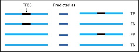
Figure 3 shows that TP is where the region (100 bp symmetric margins on both sides of TFBS) is correctly classified as a TF-binding region; FP is where the region is incorrectly classified as a TF-binding region; true negative (TN) is where the region is correctly identified as a non-TF binding region; and FN is where the region is incorrectly identified as a non-TF-binding region. Sensitivity, or true positive rate (TPR), and specificity (SPC), or true negative rate, are defined as follows:$TPR = TP/(TP+FN)$$SPC = TN/(TN+FP)$Lastly, the Matthew correlation coefficient (MCC) [52] is computed using the following formula:$\frac{TP\times TN-FP\times FN}{\sqrt{(TP+FP(FP+FN\left)\right(TN+FP\left)\right(TN+FN)}}$MCC produces a value in the range of [−1, 1], in which 1 indicates a perfect prediction, 0 means random prediction, and −1 represents a negative correlation.

Figure 3. Visual description of true positives (TP), false positives (FP), false negatives (FN) and true negatives (TN) on binding and non-binding regions in prediction. The black region indicates binding sites and the blue stretch indicates DNA region.

Hardware specifications

For the simulation, all the individual motif discovery tools in DeepFinder ran on Intel Core i5, 1.7 GHz CPU with 16 GB of memory.

Results and discussion

We investigated the performance of DeepFinder by comparing it with the original implementation of the three-stage approach. All tools used the datasets listed in Table 1 for the evaluation. For the three-stage approach, MAST [15] and FIMO [15] were used as site detection tools in stage 3, while MEME was used for initial motif prediction. The top three motifs obtained from 20% of the randomly selected input sequences were used to detect binding sites in the remaining input subset. The top motifs were chosen based on the ranking function used in MEME.

Tables 2 and 3 show the comparison results between DeepFinder, MAST and FIMO. The values in the tables are averaged scores from five-fold cross-validation. The comparison of these three models revealed that MAST consistently performed the worst in all of the evaluation metrics. FIMO is slightly better than DeepFinder in terms of precision and false discovery rate for ELK1, GATA1, P300 and SRF datasets. It is worth noticing that DeepFinder outperformed others for recall, f-measure and accuracy rates for all the datasets. For example, the recall rates for DeepFinder are >0.90 for all datasets, whereas those for FIMO averaged at 0.68 at best. However, MAST and FIMO, both have no true negatives because of the scanning upon positive controls; therefore, no specificity rates are shown.

Table 2. Comparison of average precision and the recall and f-measure rates of MAST, FIMO and DeepFinder (DF) using five-fold cross validation.

	Precision			Recall			f-measure
TF	MAST	FIMO	DF	MAST	FIMO	DF	MAST	FIMO	DF
CREB	0.60	0.99	1.00	0.03	0.45	0.97	0.06	0.62	0.99
ELK1	0.69	0.99	0.91	0.04	0.54	0.91	0.08	0.70	0.90
GATA1	0.68	0.99	0.95	0.04	0.53	0.94	0.08	0.69	0.95
HNF4	0.68	1.00	1.00	0.05	0.51	0.99	0.09	0.67	1.00
MEF2	0.80	1.00	1.00	0.01	0.20	0.98	0.03	0.33	0.99
NFE2	0.73	1.00	1.00	0.03	0.36	0.99	0.06	0.52	1.00
P53	0.71	0.99	1.00	0.05	0.49	0.99	0.09	0.66	0.99
P300	0.65	0.99	0.98	0.06	0.68	0.96	0.11	0.80	0.97
SRF	0.75	1.00	0.98	0.03	0.37	0.99	0.06	0.51	0.98
STAT1	0.67	1.00	1.00	0.04	0.44	0.99	0.07	0.61	0.99

Table 3. Comparison of false discovery rate (FDR), accuracy, and Matthews correlation coefficient (MCC) of MAST, FIMO, and DeepFinder (DF).

	FDR			Accuracy			MCC
TF	MAST	FIMO	DF	MAST	FIMO	DF	MAST	FIMO	DF
CREB	0.40	0.01	0.00	0.03	0.45	0.99	-0.62	-0.06	0.97
ELK1	0.31	0.01	0.09	0.04	0.54	0.89	-0.54	-0.05	0.81
GATA1	0.32	0.01	0.05	0.04	0.53	0.94	-0.55	-0.05	0.89
HNF4	0.32	0.00	0.00	0.05	0.51	1.00	-0.55	-0.04	0.99
MEF2	0.20	0.00	0.00	0.01	0.99	0.99	-0.44	-0.04	0.98
NFE2	0.27	0.00	0.00	0.03	0.36	1.00	-0.51	-0.03	0.99
P53	0.29	0.01	0.00	0.05	0.49	0.99	-0.53	-0.06	0.99
P300	0.35	0.01	0.02	0.06	0.67	0.97	-0.57	-0.05	0.94
SRF	0.25	0.00	0.02	0.03	0.37	0.98	-0.49	-0.03	0.96
STAT1	0.33	0.00	0.00	0.03	0.44	0.99	-0.56	-0.04	0.99

Table 3 illustrates the MCC values of the three tools. It is observed that the MCC values of DeepFinder are >0.8, which indicates a positive correlation between the predicted and the actual classes. In contrast, the MCC values of MAST and FIMO are negative for all the datasets, which indicates a poor correlation between the predicted and actual classes. In particular, FIMO MCC values are mostly near to 0, implying very poor prediction.

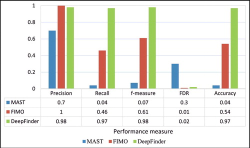
Figure 4 depicts the average f-measure, precision, recall and accuracy rates for all datasets produced by DeepFinder. It is clearly shown that ELK1 and GATA1 datasets have lower performance than that of the other datasets. Figure 5 shows the overall performance of the three tools for the three performance metrics, precision rate, recall rate and FDR. It can be observed that DeepFinder outperformed MAST and FIMO in overall results for the ten datasets. For example, the average rate obtained by DeepFinder for the ten datasets was 0.97, whereas those obtained by MAST and FIMO were 0.04 and 0.46, respectively. Likewise, DeepFinder outperformed considerably in terms of average accuracy rate of 0.97 in comparison with only 0.04 and 0.54 by MAST and FIMO, respectively. FIMO performed marginally better than DeepFinder in terms of precision rate and FDR. MAST consistently performed the worst in all the datasets and performance metrics.

Figure 4. Average f-measure, precision, recall and accuracy rates obtained by DeepFinder on the ten datasets using five-fold cross-validation.

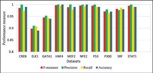
Figure 5. Average precision, recall, f-measure, false discovery rate (FDR) and accuracy for MAST, FIMO and DeepFinder for the ten datasets.

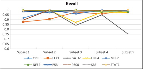
The precision and recall rates obtained by DeepFinder by using five different subsets of each dataset are presented in Figures 6 and 7. SRF dataset has rather inconsistent precision and recall rates when different subsets are used. For example, it is observed that there is a sharp decrease in the precision and recall rates when subset 2 and 5 were used. In general, the performance was quite robust when different input subsets were used for initial motif prediction. This result supported our assumption that the same set of motif features occur quite consistently across different subsets of input sequences.

Figure 6. Comparisons of precision rates for five different data subsets used in prediction.

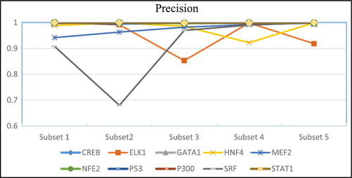
Figure 7. Comparisons of recall rates for five different data subsets used in prediction.

DeepFinder showed promising results in our evaluation using the ten datasets listed in Table 1. It demonstrates that using supervised learning with sequence content feature improves the performance of the three-stage approach. DeepFinder has better predictive power, compared to those of MAST and FIMO, particularly for TFs that bind within the enhancer regions. The improved performance is due to better representation of features associated with binding sites and the ability of supervised neural network to effectively learn the features. The 76 features were selected based on scientific evidence in the literature to represent the specificity of transcription factor proteins. Better representation improves the robustness of the motif model to noises in the final site detection stage. In addition, the multi-layer structure of the neural network coupled with supervised learning can effectively learn the input-output mapping. The strength of the neural network is in its ability to learn different abstractions of features through different configurations of the number of hidden layers and hidden neurons in each layer [53]. Our results suggest that a motif model obtained from supervised learning has better discriminative power compared with the PWM. The use of multiple tools for initial prediction in the first stage increases the chances of obtaining true binding sites. The poor performance of MAST and FIMO is inherited from the performance level of MEME as well as the binding model used. It is known that the PWM binding model is poor in capturing sequence specificities of various TFs [14,54]. It is seen in Table 2 that FIMO achieved a slightly higher precision rate in three of the ten datasets (i.e. ELK1, GATA1, SRF) compared with DeepFinder. Upon checking the consensus motif patterns of those datasets, it is observed that they are highly conserved, while for the CREB and the p53, which have less conserved motif patterns, DeepFinder performed better than FIMO. Although this explanation is far from conclusive with the limited datasets evaluated, it is safe to infer that one of DeepFinder's strengths lies in better modelling the specificity of less conserved motifs.

Conclusions

We have proposed the DeepFinder framework, a simple yet effective ensemble method that utilizes positive information in the motifs returned by multiple motif discovery tools for motif identification purposes. Overall, our solution produced highly improved results in comparison with the original implementation of the three-stage approach. Our solution, which incorporated sequence content feature and deep learning, demonstrates promising potential for modeling TF specificities. The various sequence features used are effective in representing the salient characteristics of binding sites in comparison with PWM. In addition, our results also suggest an effective implementation of the three-stage approach for tackling large input datasets. Using DeepFinder has several advantages. First, stacked autoencoder employed in DeepFinder can accurately predict regulatory sequences without any prior knowledge about transcription factor binding sites (e.g. lengths of possible motifs and pre-fixed motif model) by using only sequence content information for model construction. Second, DeepFinder is flexible to capitalize novel feature information related to binding sites in the future. The new features can be easily used as inputs to the DeepFinder for more effective motif modeling. Third, deep learning neural networks is known to learn better when more data are available. While large data are not a requirement for DeepFinder, we can expect it to perform better when larger subsets are used. However, PWM is restricted by the number of free parameters that are pre-defined in the model. This implies that more data would not necessarily increase the amount of information it can represent. For the future studies, one of the pertinent issues is the representation of DNA sequences for other types of deep learning neural networks such as CNN. CNN is powerful because it can learn the different abstraction of features in DNA sequences without the need of handcrafted features. However, it requires DNA sequences to be represented as vectors or in the matrix form (i.e. as an image) for effective learning. The currently available solution mainly focuses on one-hot encoding, which we feel is not a ‘natural’ representation of DNA sequences. We are currently conducting exploratory research for more meaningful representation of DNA sequences as ‘images.’ In addition, a more effective method is needed to merge and filter large number of candidate motifs from multiple motif prediction tools.

Acknowledgements

YS is supported by the Malaysian MyBrain15 MyPhD Scholarship. ON is supported by the Fundamental Research Grant Scheme FRGS/1/2014/SG03/UNIMAS/02/2.

Disclosure statement

No potential conflict of interest was reported by the authors.

Additional information

Funding

This study was supported by the Malaysia Research Acculturation Grant Scheme of the Ministry of Higher Education Malaysia [grant number RAGS/b(5)/927/2012(28)].

References

- Maston GA, Evans SK, Green MR. Transcriptional regulatory elements in the human genome. Annu Rev Genomics Hum Genet. 2006;7:29–59.
- Zambelli F, Pesole G, Pavesi G. Motif discovery and transcription factor binding sites before and after the next-generation sequencing era. Brief Bioinform. 2013;14:225–237.
- Poliakov A, Foong J, Brudno M, et al. GenomeVISTA—an integrated software package for whole-genome alignment and visualization. Bioinformatics. 2014;30:2654–2655.
- Brudno M, Do CB, Cooper GM, et al. LAGAN and Multi-LAGAN: efficient tools for large-scale multiple alignment of genomic DNA. Genome Res. 2003;13:721–731.
- Kurtz S, Phillippy A, Delcher AL, et al. Versatile and open software for comparing large genomes. Genome Biol. 2004 [cited 2017 Mar 12];5:R12. DOI:10.1186/gb-2004-5-2-r12
- Bray N, Dubchak I, Pachter L. AVID: A global alignment program. Genome Res. 2003;13:97–102.
- Ovcharenko I, Loots GG, Giardine BM, et al. Mulan: multiple-sequence local alignment and visualization for studying function and evolution. Genome Res. 2005;15:184–194.
- Smith TF, Waterman MS. Identification of common molecular subsequences. J Mol Biol. 1981;147:195–197.
- Needleman SB, Wunsch CD. A general method applicable to the search for similarities in the amino acid sequence of two proteins. J Mol Biol. 1970;48:443–453.
- Blanchette M, Kent WJ, Riemer C, et al. Aligning multiple genomic sequences with the threaded blockset aligner. Genome Res. 2004;14:708–715.
- Al Ait L, Yamak Z, Morgenstern B. DIALIGN at GOBICS–multiple sequence alignment using various sources of external information. Nucleic Acids Res. 2013;41:W3–7.
- King DC, Taylor J, Zhang Y, et al. Finding cis-regulatory elements using comparative genomics: some lessons from ENCODE data. Genome Res. 2007;17:775–786.
- Kel AE, Gössling E, Reuter I, et al. MATCH: A tool for searching transcription factor binding sites in DNA sequences. Nucleic Acids Res. 2003;31:3576–3579.
- Wang D, Lee NK. MISCORE: Mismatch-based matrix similarity scores for DNA motif detection. In: Köppen M, Kasabov N, Coghill G, editors. Adv. Neuro-Information Process. Berlin, Heidelberg: Springer; 2009. p. 478–485.
- Grant CE, Bailey TL, Noble WS. FIMO: scanning for occurrences of a given motif. Bioinformatics. 2011;27:1017–1018.
- Bailey T, Boden M, Whitington T, et al. The value of position-specific priors in motif discovery using MEME. BMC Bioinformatics. 2010 [cited 2017 Mar 12];11:179. DOI:10.1186/1471-2105-11-179.
- Stormo GD. DNA binding sites: representation and discovery. Bioinformatics. 2000;16:16–23.
- Bi Y, Kim H, Gupta R, et al. Tree-based position weight matrix approach to model transcription factor binding site profiles. PLoS One. 2011 [cited 2017 Mar 12];6:e24210. DOI:10.1371/journal.pone.0024210.
- Bailey TL, Gribskov M. Combining evidence using p-values: application to sequence homology searches. Bioinformatics. 1998;14:48–54.
- Osada R, Zaslavsky E, Singh M. Comparative analysis of methods for representing and searching for transcription factor binding sites. Bioinformatics. 2004;20:3516–3525.
- Hu J, Li B, Kihara D. Limitations and potentials of current motif discovery algorithms. Nucleic Acids Res. 2005;33:4899–4913.
- Hughes JD, Estep PW, Tavazoie S, et al. Computational identification of Cis-regulatory elements associated with groups of functionally related genes in Saccharomyces cerevisiae. J Mol Biol. 2000;296:1205–1214.
- Bailey TL, Elkan C. Fitting a mixture model by expectation maximization to discover motifs in biopolymers. Proc Int Conf Intell Syst Mol Biol. 1994;2:28–36.
- Liu XS, Brutlag DL, Liu JS. BioProspector: discovering conserved DNA motifs in upstream regulatory regions of co-expressed genes. Pacific Symp Biocomput. 2001;6:127–138.
- Thijs G, Marchal K, Lescot M, et al. Gibbs sampling method to detect overrepresented motifs in the upstream regions of coexpressed genes. J Comput Biol. 2002;9:447–464.
- Liu XS, Brutlag DL, Liu JS. An algorithm for finding protein-DNA binding sites with applications to chromatin-immunoprecipitation microarray experiments. Nat Biotechnol. 2002;20:835–839.
- Pavesi G, Mauri G, Pesole G. An algorithm for finding signals of unknown length in DNA sequences. Bioinformatics. 2001;17:S207–214.
- Wei Z, Jensen ST. GAME: detecting cis-regulatory elements using a genetic algorithm. Bioinformatics. 2006;22:1577–1584.
- Fogel GB, Weekes DG, Varga G, et al. Discovery of sequence motifs related to coexpression of genes using evolutionary computation. Nucleic Acids Res. 2004;32:3826–3835.
- Bailey TL. DREME: motif discovery in transcription factor ChIP-seq data. Bioinformatics. 2011;27:1653–1659.
- Shi J, Yang W, Chen M, et al. AMD, an automated motif discovery tool using stepwise refinement of gapped consensuses. Aiyar A, editor. PLoS One. 2011 [cited 2017 Mar 12];6:e24576. DOI:10.1371/journal.pone.0024576.
- Lee NK, Fong PK, Abdullah MT. Modelling complex features from histone modification signatures using genetic algorithm for the prediction of enhancer region. Bio-Medical Mater Eng. 2014;24:3807–3814.
- Zia A, Moses AM. Towards a theoretical understanding of false positives in DNA motif finding. BMC Bioinformatics. 2012 [cited 2017 Mar 12];13:151. DOI:10.1186/1471-2105-13-151.
- Thomas-Chollier M, Herrmann C, Defrance M, et al. RSAT peak-motifs: motif analysis in full-size ChIP-seq datasets. Nucleic Acids Res. 2012 [cited 2017 Mar 12];40:e31. DOI:10.1093/nar/gkr1104.
- Li L. GADEM: A genetic algorithm guided formation of spaced dyads coupled with an EM algorithm for motif discovery. J Comput Biol. 2009;16:317–329.
- Kuttippurathu L, Hsing M, Liu Y, et al. CompleteMOTIFs: DNA motif discovery platform for transcription factor binding experiments. Bioinformatics. 2011;27:715–717.
- Carroll JS, Meyer CA, Song J, et al. Genome-wide analysis of estrogen receptor binding sites. Nat Genet. 2006;38:1289–1297.
- Wei C-L, Wu Q, Vega VB, et al. A global map of p53 transcription-factor binding sites in the human genome. Cell. 2006;124:207–219.
- Lee NK, Wang D. Optimization of MISCORE-based motif identification systems. 3rd International Conference on Bioinformatics and Biomedical Engineering (ICBBE 2009); 2009; Beijing, China.
- Alipanahi B, Delong A, Weirauch MT, et al. Predicting the sequence specificities of DNA-and RNA-binding proteins by deep learning. Nat Biotechnol. 2015;33:831–838.
- Quang D, Xie X. DanQ: a hybrid convolutional and recurrent deep neural network for quantifying the function of DNA sequences. Nucleic Acids Res. 2016 [cited 2017 Mar 12];44:e107. DOI:10.1093/nar/gkw226.
- Sun H, Yuan Y, Wu Y, et al. Tmod: toolbox of motif discovery. Bioinformatics. 2010;26:405–407.
- de Hoon MJL, Imoto S, Nolan J, et al. Open source clustering software. Bioinformatics. 2004;20:1453–1454.
- Wijaya E, Yiu S-M, Son NT, et al. MotifVoter: a novel ensemble method for fine-grained integration of generic motif finders. Bioinformatics. 2008;24:2288–2295.
- Yáñez-Cuna JO, Arnold CD, Stampfel G, et al. Dissection of thousands of cell type-specific enhancers identifies dinucleotide repeat motifs as general enhancer features. Genome Res. 2014;24:1147–1156.
- Vincent P, Larochelle H, Bengio Y, et al. Extracting and composing robust features with denoising autoencoders. In: Proceeding of 25th International Conference on Machine Learning; 2008. p. 1096–1103. New York, NY: ACM.
- Giardine B, Riemer C, Hardison RC, et al. Galaxy: a platform for interactive large-scale genome analysis. Genome Res. 2005;15:1451–1455.
- Palm RB. Deep learning toolbox. [2015-09]. http://www.mathworks.com/matlabcentral/fileex-change/38310-deep-learning-toolbox. 2012.
- Rosenbloom KR, Armstrong J, Barber GP, et al. The UCSC Genome Browser database: 2015 update. Nucleic Acids Res. 2015;43:D670–D681.
- Manning CD, Raghavan P, Schütze H, et al. Introduction to information retrieval. Cambridge: Cambridge University Press; 2008.
- Benjamini Y, Hochberg Y. Controlling the false discovery rate: a practical and powerful approach to multiple testing. J R Stat Soc Ser B. 1995; 57:289–300.
- Matthews BW. Comparison of the predicted and observed secondary structure of T4 phage lysozyme. Biochim Biophys Acta (BBA)-Protein Struct. 1975;405:442–451.
- Haykin S. Neural networks: A comprehensive foundation. 2nd ed. Upper Saddle River (NJ, USA): Prentice Hall PTR; 1998.
- Wasserman WW, Sandelin A. Applied bioinformatics for the identification of regulatory elements. Nat Rev Genet. 2004;5:276–287.