A hierarchical multi-label classification method based on neural networks for gene function prediction

abstract

Gene function prediction is used to assign biological or biochemical functions to genes, which continues to be a challenging problem in modern biology. Genes may exhibit many functions simultaneously, and these functions are organized into a hierarchy, such as a directed acyclic graph (DAG) for Gene Ontology (GO). Because of these characteristics, gene function prediction can be seen as a typical hierarchical multi-label classification (HMC) task. A novel HMC method based on neural networks is proposed in this article for predicting gene function based on GO. The proposed method belongs to a local approach by transferring the HMC task to a set of subtasks. There are three strategies implemented in this method to improve its performance. First, to tackle the imbalanced data set problem when building the training data set for each class, negative instances selecting policy and SMOTE approach are used to preprocess each imbalanced training data set. Second, a particular multi-layer perceptron (MLP) is designed for each node in GO. Third, a post processing method based on the Bayesian network is used to guarantee that the results are consistent with the hierarchy constraint. The experimental results indicate that the proposed HMC-MLPN method is a promising method for gene function prediction based on a comparison with two other state-of-the-art methods.

Keywords:

• Gene function prediction
• gene ontology
• hierarchical multi-label classification
• neural network

Introduction

Research on gene function is of great significance in the development of new drugs, better crops and even synthetic biochemical compounds [1]. A large amount of functional genomic data has been accumulated, and manual analysis of these instrumental data is tedious and cumbersome. Thus, machine learning approaches have been used to solve this problem, by considering the gene function prediction problem as a classification task. As a single gene may have many functions that are structured according to a predefined hierarchy [2], the gene function prediction problem naturally belongs to the hierarchical multi-label classification (HMC) problems [3]. In the HMC problem, classes are organized in a predefined hierarchical structure [4], and an instance can be assigned with a set of classes [5]. Particularly, an instance can be assigned to classes that belong to the same hierarchical level at the same time. For gene functional classes, there are two main hierarchy structures [6]: a directed acyclic graph (DAG) for Gene Ontology (GO) and a rooted tree for Functional Catalogue (FunCat). In a tree structure, each class node has only one parent node; however, in the DAG structure, a class node can have multiple parent nodes [7]. Due to the fact the DAG structure is more complicated, most studies have usually dealt with tree structures in the past, and only a few studies have used the DAG of GO. Currently, GO has become the most popular functional classification scheme for gene function prediction studies, so our work focuses on GO taxonomy.

The Gene Ontology is a typical protein function classification scheme comprising thousands of functional classes structured as a DAG hierarchy of terms, in which each term corresponds to a functional class [8]. GO covers three different domains, so it can be divided into three DAG-structured ontologies: biological process, molecular function and cellular component [9]. A small subset of GO is shown in Figure 1.

Figure 1. A fraction of the GO taxonomy. Reprinted from [24].

Published HMC methods can be categorized into two groups: global approaches and local approaches [10]. The global approach generates a single model that predicts all classes of an instance by running the classification algorithm once [11]. The algorithm proposed in [12] is a representative global approach. In contrast, a binary classifier is trained for each class independently in the local approach, and then an additional step is usually used to combine these separate results by considering the hierarchy [13]. The complicated HMC task is decomposed into a group of subtasks, which can be easily solved by conventional binary classification algorithms.

When using the local approach to solve the HMC problem, two key points need to be considered carefully. The first one is that the HMC task is an imbalanced data set learning scenario, and the minority class is usually neglected by binary classifiers [14]. As the classes are organized as a hierarchy, the training data sets for the classes at lower levels are usually very skewed because there are fewer positive instances in these data sets [15]. Second, the prediction result must be consistent with the hierarchy constraint. That is, an instance should automatically belong to all ancestor classes of the class to which it belongs; and should not belong to any of the descendant classes of the class to which it does not belong [16].

Most existing methods belong to the local approach, such as the methods proposed in [17–21]. Only a few HMC methods among them can address GO, which has a more complicated DAG structure. However, GO is now the most popular functional classification scheme for gene function prediction studies, and thus the focus of our present study is to classify the DAG structure of the GO taxonomy. In paper [22], a local HMC approach called HMC-LMLP is proposed. It trains separate Multi-Layer Perceptrons (MLPs) for each given level of the hierarchy, and the top-down method is chosen to correct inconsistencies of final predictions. When tackling the DAG structure, the DAG structure needs to be transformed to a tree structure, which may lead to loss of some information of the original hierarchy. A deep neural network architecture HMCN proposed in paper [23] also needs to reduce the DAG to a tree structure, which may also suffer the problem of losing hierarchical information. In our previously published paper [24], SVM is chosen as the base classifier.

Compared to these previous works, in the present paper, we propose the hierarchical HMC with MLP per node (HMC-MLPN) method for the gene function prediction problem based on GO. Specifically, we make the following contributions. First, a MLP is designed for each node in the GO taxonomy. Second, the imbalanced training data sets problem is alleviated by both the sibling policy and the SMOTE method [25]; and third, the nodes interaction method is proposed to guarantee the hierarchy constraint for the final result. These techniques together improve the final predictions of gene function. We perform experiments to evaluate the performance of the algorithm using eight benchmark data sets and compare it with state-of-the-art algorithms. Our experimental results show that HMC-MLPN performs better than these existing algorithms.

Methods

Notation and basic definitions

The notations and definitions used here were previously described in detail [24]. Briefly, a gene instance x_i with m attributes is written as x_i = (a_i1, a_i2,…, a_im), x_i ϵ X, (1≤ i ≤ n), where X denotes the gene instance set. Let C be a set of all GO classes, C= {c₁, c₂,…,c_|C|}. The hierarchy of GO is a DAG, and it is denoted by G = <V, E>. V= {1, 2,…, |V|} and E are the sets of vertices and edges, respectively. Each node in V represents a gene function class, so V = C and the class c_k is represented simply by the node k if there is no ambiguity. A direct edge e = (k,l) ϵ E means that k is the parent node of l in G. If an instance x_i ϵ X has the function of the node k, the real label at this node is 1. If there is no ambiguity, it is said its node k is 1 for short. For an instance x_i, the preliminary score d*_i = (d*,_i1 d*,_i2…, d*_i|C|) is provided a set of |C| binary classifiers. d*_ik is the probability P*_i (k = 1) given by the classifier f_k at the node k. Similarly, d_ik represents the final predicted score at the node k. Predicted labels y*_i = (y*_i1, y*_i2,…, y*_i|C|) and y_i = (y_i1, y_i2,…, y_i|C|) are obtained by selecting a threshold θ for predicted scores d*_i and d_i. For example, if d*_ik ≥ θ, set y*_ik =1, otherwise set y*_ik = 0 for 1≤ k ≤ C.

The main processes of HMC-MLPN

The HMC-MLPN algorithm belongs to the local approach, and the rationale behind it is that each MLP may employ different local information and that the complicated learning process is replaced by multiple simple processes. There are three steps in the proposed algorithm, which are described as follows. The first step is the data set preprocessing step. In this step, |C| different training data sets for each node are built by utilizing a negative instance selecting policy, where |C| means the total number of all classes in GO. Each training data set is also modified by the over-sampling technique to change the data distribution. This procedure can alleviate the imbalanced data set problem. Then, in the second step, |C| neural networks, which are also called base classifiers or local classifiers, are trained by using these training data sets. The final step is the prediction step. In the prediction phase, the instances in the test set are first predicted by |C| neural networks. Subsequently, these preliminary prediction results are combined by the nodes interaction method to ensure the hierarchy constraint.

Training data set preprocessing

The method to build a suitable training data set for a classifier is very important. Usually, if the number of positive instances and the number of negative instances in a data set are nearly the same, the classifier can potentially achieve good performance on this data set. For the GO hierarchy, the classes are organized as a DAG structure. Nearly all the instances belong to the classes at the top of the hierarchy. From the top to the bottom of the hierarchy, the number of instances belonging to the class drops significantly, and the fewest instances are annotated to the classes at the lowest level. There is a great difference in the quantity of positive instances and negative instances for some classes, and this case is called an imbalanced data set problem. This problem leads to difficulty in accurate predictions for standard classifiers, since the minority class tends to be overwhelmed by the majority one and classifiers need to be learned from strongly skewed training data sets [26].

To alleviate the imbalanced data set problem, the sibling policy is selected to build the training data set, which is recommended in [27]. This policy explores the hierarchical structure of GO and can reduce the number of negative instances for some classes. To be specific, for a class k, only instances belonging to the siblings of k are selected as negative instances [28].

The training data sets remain imbalanced in some classes, even though the sibling policy has been applied. To solve this problem, we use the SMOTE method to add some minority instances artificially to each training data set. The SMOTE method described in [25], is an efficient re-sampling approach. By producing new synthetic instances for minority classes, it can change the distribution of the training data set and further change the decision domain of a classifier.

Neural network training

In this algorithm, an individual MLP is trained for each node in the GO. The hypothesis is that different patterns and local information can be extracted from instances at different nodes, so each MLP can learn something different from the others [29]. This step divides the complicated learning process into a set of simple subprocesses. Figure 2 presents the architecture of this step, and the details of the training process are described as follows. In the figure, X is a training sample, and H_1i and H_2i are the hidden layers. O_i is the output layer of the neural network associated with node i, and O_all means the merged output vector for all the nodes, where O_all = (O₁, O₂,…, O_|C|). The weight matrix W_1i represents the weights connecting the input attributes and the neurons in the first hidden layer. Similarly, W_1i, W_2i, and W_3i represent the activations of the first hidden layer with the neurons in the second hidden layer; and the activations in the second hidden layer with the neurons in the output layer of the MLP associated with node i.

Figure 2. Architecture of each MLP.

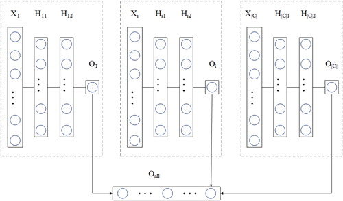
In this algorithm, each node is associated with an MLP with two hidden layers. The input for each neural network is the feature vector of each sample, and the output neuron is associated with the class of the corresponding node. A binary crossentropy loss function is used in each MLP. For performing parameter updating, each MLP makes use of AdaGrad as the optimizer, and the reason is that AdaGrad converges faster than SGD. To avoid the overfitting problem, we perform dropout regularization, which stochastically disables a percentage of neurons in each hidden layer.

As can be observed in the figure, the training process of the MLP is repeated for each node in GO, and it can be performed in parallel, which can speed up the training process. Considering the computational cost, each MLP has a complexity of O (W_i), with (W_i) being the number of weights and biases of the neural network associated with node i. Assume that A is the number of attributes in the data set, H_1i and H_2i are the number of neurons in the first and second hidden layers of the neural network associated with node i, and O_i is the number of output neurons of the neural network associated with node i. We can then define (W_i) as (A + 1) × H_1i + H_1i +1) × H_2i + (H_2i +1) × O_i. The overall training cost of each neural network associated with node i is then O (W_i) × m× n), with m being the number of training objects and n being the number of training epochs.

Prediction

When making predictions, |C| neural networks give the probabilistic preliminary results for unknown instances firstly. Because these neural networks are trained separately, it is possible that an instance x_i is predicted to have a class k according to its preliminary result calculated by the MLP at this node, but x_i does not have the parent classes of k. It means that these preliminary results violate the hierarchy constraint, which is also called the TPR rule [30]. When such a case occurs, we used the nodes interaction method to ensure that the final results are consistent with the hierarchy constraint.

The nodes interaction method proposed in [24] is a post processing method. As previously described, in this method, the hierarchical interaction between a node and its adjacent nodes in GO are considered based on the Bayesian network when making final prediction decisions [31]. There are two phases in the nodes interaction method: a preliminary results correction phase and a final decision determination phase. The effect of the first phase is that the hierarchical relationship between nodes can influence the predicted result for a node. As the nodes of the GO are organized as a DAG, a Bayesian network is utilized in this phase, which is described as follows.

For an instance x_i, its prior probability at node k is P*_i (k = 1) = d*_ik. When calculating the posterior probability P (k = 1), the influence of its parent nodes par(k) and children nodes child(k) are considered separately. To consider the parent nodes part of a node k, the posterior probability P (k = 1) is written as P_par (k = 1), which is calculate as $P^{*}(k=1){\prod }_{j\in par(k)}{P}^{*}(j=1)$, and P_par (k = 0) is derived by 1-P_par (k = 1). Similarly, when considering the children nodes part, the posterior probability P_child (k = 0) can be calculated by $P^{*}(k=0){\prod }_{j\in par(k)}{P}^{*}(j=0)$, and P_child (k = 1) is 1-P_child (k = 0).

Between two probabilities P_par(k = 0) and P_child(k = 1), the bigger one is selected as the value of P(k = 1). More precisely, for a node k, let ${\overline{d}}_k$

be the result P (k = 1) in this phase. When P_par (k = 0) is not less than P_child (k = 1), ${\overline{d}}_k$ is equal to P_par (k = 0), otherwise, ${\overline{d}}_k$ is assigned as P_child (k = 1).

The influence of a node's parent and children nodes is considered in the preliminary results correction phase, but this step cannot ensure that the final results are consistent with the hierarchy constraint. The final decision determination phase modifies the preliminary results by propagating negative decisions towards the child nodes from the top to the bottom of the DAG. Let ${\overline{d}}_k$ be the prediction calculated in the first phase, then the final result $d_k$ for the node k is calculated as follows: (1) $$d_k=\{\begin{array}{c}{\overline{d}}_k,\\ \underset{j\in par\left(k\right)}{\min }{d}_j,\\ {\overline{d}}_k,\end{array}\begin{array}{c}if k is \mathit{\text{root}} \mathit{\text{node}}\\ if {\overline{d}}_k>\underset{j\in par\left(k\right)}{\min }{d}_j\\ \mathit{\text{otherwise}}\end{array}$$(1)

Data

This study used standard data sets for Saccharomyces cerevisiae downloaded from the DTAI website¹. Saccharomyces cerevisiae (baker's or brewer's yeast) is a typical model organism. It has been studied by many researchers, and extensive data are available. Among the present studies, most researchers selected the same group of data to predict gene functions because it is easy to evaluate the results of different methods. These data sets describe phenotypes and gene expression, and each data set describes a different aspect of the genes in the yeast genome. More details can be found in [12]. In this research, we also chose this group of data sets and annotated them with GO. The GO file and GO annotation (GOA) file of Yeast were downloaded from the GO website and the European Bioinformatics Institute [32]. The main characteristics of the group of data sets, including their instance number, attribute number, and number of GO terms are listed in Table 1.

Table 1. The characteristics of the experimental data sets.

Data set	Attributes	Training instances	Testing instances	Number of GO terms
D1 Cellcycle	77	2290	1202	168
D2 eisen	79	2252	1182	125
D3 derisi	63	1537	817	165
D4 gasch1	173	2294	1205	168
D5 gasch2	52	1301	1212	168
D6 church	27	2289	1202	168
D7 spo	80	2354	1183	165
D8 seq	478	2321	1225	168

As previously described [12], we use two-thirds of each data set for training and the remaining one-third for testing. Out of the training set, two-thirds are used for the actual training and one-third is used to validate the parameters [33]. Missing values of some features are replaced with the mean of the non-missing values. The GO file and GOA file of Yeast were downloaded from the GO website and the European Bioinformatics Institute [32]. We processed the GO file and GOA file according to the recommendations in paper [34]. The biological process aspect of GO is our focus in the experiment section.

Results and discussion

Experimental parameters

We use a learning rate of 0.01, є=10⁻⁶, and dropout of 0.5. The activation function for the hidden layers is ReLU function, and is a logistic sigmoid function for the output layer, so the output of each MLP is a probability value. The number of neurons in each layer is defined by (m + 1)/2, where m is the attribute number of the instance. For example, for the Cellcycle data set, the attribute number is 77, that is, there are (77 + 1)/2 = 39 neurons in each hidden layer. These neural networks are trained by optimizing the binary crossentropy error.

Evaluation metrics

To date, although some evaluation measures have been proposed, no hierarchical classification measure can be considered to be the best among all possible hierarchical classification scenarios and applications. Following the suggestions in paper [27], hierarchical precision (hPre), hierarchical recall (hRec) and hierarchical F₁ (hF₁) are used as evaluation measures for the experiments. There are two versions of these evaluation metrics, a micro-averaging version and a macro-averaging version [35].

For an instance i, let $P_i^{̂}$ be the set consisting of all the predicted labels, and $T_i^{̂}$ be the set consisting of all true labels. For the micro-averaging version of hierarchical precision, recall, and F₁ are defined as follows: (2) $$hPr{e}^{\mu }=\frac{\sum _{i=1}^n|{\widehat{P}}_i\cap {\widehat{T}}_i|}{\sum _{i=1}^n\left|{\widehat{P}}_i\right|}$$(2) (3) $$hRe{c}^{\mu }=\frac{\sum _{i=1}^n|{\widehat{P}}_i\cap {\widehat{T}}_i|}{\sum _{i=1}^n\left|{\widehat{T}}_i\right|}$$(3) (4) $$h{F}_1{}^{\mu }=\frac{2\times hPr{e}^{\mu }\times hRe{c}^{\mu }}{hPr{e}^{\mu }+hRe{c}^{\mu }}$$(4)

For the macro-averaging version, hierarchical precision, recall and F₁ are first computed for each instance i, and then these results for each instance are averaged to obtain the macro-averaging version metrics as follows: (5) $$hPr{e}^M=\frac{\sum _{i=1}^n\frac{|P_i^{̂}\cap T_i^{̂}|}{\left|P_i^{̂}\right|}}{n}$$(5) (6) $$hRe{c}^M=\frac{\sum _{i=1}^n\frac{|P_i^{̂}\cap T_i^{̂}|}{\left|T_i^{̂}\right|}}{n}$$(6) (7) $$h{F}_1{}^{\mu }=\frac{\sum _{i=1}^n\frac{2\times \frac{|P_i^{̂}\cap T_i^{̂}|}{\left|P_i^{̂}\right|}\times \frac{|P_i^{̂}\cap T_i^{̂}|}{\left|T_i^{̂}\right|}}{\frac{|P_i^{̂}\cap T_i^{̂}|}{\left|P_i^{̂}\right|}+\frac{|P_i^{̂}\cap T_i^{̂}|}{\left|T_i^{̂}\right|}}}{n}$$(7)

Experiment results and analysis

The HMC-MLPN algorithm is proposed to predict gene function based on GO. In this section, the predictive performance of the proposed algorithm compared with other state-of-the-art methods is given. Due to the complexity of GO with DAG structure, only a few algorithms have been proposed previously. After analyzing the existing literature, two state-of-the-art methods along with the previous method proposed in paper [24] were selected as methods for comparison because of their good performance and representativeness for gene function prediction.

As a representative local approach method, the TPR ensemble method outperforms the flat ensemble method and the hierarchical top-down method. Among global approach algorithms, such as HLCS-Multi, HLCS-DAG and HMC-LMLP, the CLUS-HMC method exhibits the best performance [12]. The details about these two algorithms are described in [12,18].

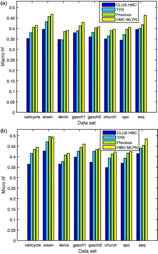
Both the macro-averaged version and micro-averaged version of hF₁ are computed to evaluate the performance of the HMC-MLPN method. The performance comparisons of different algorithms for eight data sets in terms of macro-averaged version values and micro-averaged version values are shown in Figure 3, and “previous” means the method proposed in paper [24].

hPre, hRec and hF₁ range from 0 to 1. For all these metrics, if a classifier has the largest value among all classifiers, it means that the classifier has the best performance. Ideally, both hierarchical precision and hierarchical recall are expected to be larger. However, typically, there is a negative correlation between precision and recall, so hF₁ is proposed to take into account both hPre and hRec to calculate an overall value. In Figure 3, the proposed HMC-MLPN method has the highest value on all eight data sets, which means that it has better performance than the TPR ensemble method or the CLUS-HMC method. In addition, the performance of the HMC-MLPN method is slightly better than the previous method proposed in paper [24].

Figure 3. Results of hF₁ for eight data sets: macro-averaged version (a) and micro-averaged version (b).

The good performance of the HMC-MLPN method is realized by all three steps in the algorithm together. First, compared with the CLUS-HMC method, which tackles all the data together but does not consider the relationship between the data and different nodes, the proposed HMC-MLPN method builds a balanced data set for each node, which allows the classifier to achieve better predictions. In addition, a particular MLP is designed for each node in GO. Due to the fact that the MLP has good performance in classification and that each MLP can capture local information from its respective node, the HMC-MLPN method could take advantage of the relationship between the data and nodes.

Second, although both the TPR ensemble method and the HMC-MLPN method belong to the local approach, the HMC-MLPN method’s advantage is that it employs the nodes interaction method, which can not only guarantee the hierarchy constraint but also lead to improvement of the results in the third step.

Conclusions

Gene function prediction is an important task, and a large amount of biological data must be analyzed. In this article, the HMC-MLPN method is proposed to predict gene function based on GO, which has a DAG hierarchy. Due to the particularities of GO, the HMC-MLPN method has three characteristics. First, the imbalanced data set problem is considered. When building the training data set for each class, the siblings policy and the over-sampling approach SMOTE are used. Second, an MLP with two hidden layers is designed for each node, and each neural network is responsible for the predictions at its corresponding node. Third, a nodes interaction method is proposed to combine the results of the neural networks and to ensure that the final results are consistent with the hierarchy constraint. In these experiments, the results showed that the HMC-MLPN method exhibits the best performance on all eight data sets. Thus, the HMC-MLPN method is expected to be a potential approach to solve the gene function prediction problem based on GO.

Disclosure statement

The authors declare no conflict of interest.

Additional information

Funding

This work is supported in part by the Fundamental Research Funds for the Central Universities under grant number HIT NSRIF.20169, the Heilongjiang Postdoctoral Fund under grant number LBH-Z16081, and the Online Education Research Funds of Online Education Research Center of Ministry of Education (Quantong Education) under grant number 2016YB132.

Notes

1 http://dtai.cs.kuleuven.be/clus/hmcdatasets/

References

- Meng J, Wekesa JS, Shi GL, et al. Protein function prediction based on data fusion and functional interrelationship. Math Biosci. 2016;274:25–32.
- Ricardo C, Barros RC, de Carvalho ACPLF, et al. Reduction strategies for hierarchical multi-label classification in protein function prediction. BMC Bioinform. 2016;17(1):373. DOI: 10.1186/s12859-016-1232-1
- Madjarov G, Dimitrovski I, Gjorgjevikj D, et al. Evaluation of different data-derived label hierarchies in multi-label classification. In: Appice A, Ceci M, Loglisci C, Manco G, Masciari E, Ras Z, editors. New frontiers in mining complex patterns. NFMCP. (Lecture Notes in Computer Science, vol 8983). Cham: Springer; 2014.
- Cerri R, Pappa GL, de Carvalho ACPLF, et al. An extensive evaluation of decision treebased hierarchical multilabel classification methods and performance measures. Comput Intell. 2015;31(1):1–46.
- Romo LM, Nievola JC. Hierarchical multi-label classification problems: An LCS approach. In: Omatu S, et al., editors. Distributed Computing and Artificial Intelligence, 12th International Conference; Salamanca, Spain, June; 2015 (Advances in Intelligent Systems and Computing, vol 373). Cham: Springer; 2015. p. 97–104.
- Bi W, Kwok JT. Bayes-optimal hierarchical multilabel classification. IEEE Trans Knowl Data Eng. 2015;27(11):2907–2918.
- Merschmann LHDC, Freitas AA. An extended local hierarchical classifier for prediction of protein and gene functions. In: Bellatreche L, Mohania MK, editors. Data warehousing and knowledge discovery. DaWaK 2013. (Lecture Notes in Computer Science, vol. 8057). Berlin: Springer; 2013.
- Ashburner M, Ball J Cablake, Botstein D, et al. Gene ontology: tool for the unification of biology. The Gene Ontology consortium. Nat Genet. 2000;25(1):25–29.
- Peng J, Wang T, Wang J, et al. Extending gene ontology with gene association networks. Bioinformatics. 2016;32(8):1185–1194.
- Santos A, Canuto A. Applying semi-supervised learning in hierarchical multi-label classification. Expert Syst Appl. 2014;41(14):6075–6085.
- Sun Z, Zhao Y, Cao D, et al. Hierarchical multilabel classification with optimal path prediction. Neural Process Lett. 2016;45(1):1–15.
- Vens C, Struyf J, Schietgat L, et al. Decision trees for hierarchical multi-label classification. Mach Learn. 2008;73(73):185–214.
- Zhang L, Shah SK, Kakadiaris IA. Hierarchical multi-label classification using fully associative ensemble learning. Pattern Recogn. 2017;70: 89–103.
- Otero FEB, Freitas AA, Johnson CG. A hierarchical multi-label classification ant colony algorithm for protein function prediction. Memet Comput. 2010;2(3):165–181.
- Zhengping L, Rui G, Jiangtao S, et al. Orderly roulette selection based ant colony algorithm for hierarchical multilabel protein function prediction. Math Probl Eng. 2017;2017(2):1–15.
- Stojanova D, Ceci M, Malerba D, et al. Using PPI network autocorrelation in hierarchical multi-label classification trees for gene function prediction. BMC Bioinform. 2013;4(14):3955–3957.
- Barutcuoglu Z, Schapire R, Troyanskaya O. Hierarchical multi-label prediction of gene function. Bioinformatics. 2006;22(7):830–836.
- Valentini G. True path rule hierarchical ensembles for genome-wide gene function prediction. IEEE/ACM Trans Comput Biol Bioinform. 2011;8(3):832–847.
- Chen B, Hu J. Hierarchical multi-label classification based on over‐sampling and hierarchy constraint for gene function prediction. IEEJ T Electr Electr. 2012;7(2):183–189.
- Robinson PN, Frasca M, Khler S, et al. A hierarchical ensemble method for dag-structured taxonomies. Lect Notes Comput Sci. 2015;9132:15–26.
- Cerri R, de Carvalho ACPLF, Freitas AA. Adapting non-hierarchical multilabel classification methods for hierarchical multilabel classification. Intell Data Anal. 2011;15(6):861–887.
- Cerri R, Barros RC, de Carvalho ACPLF. Hierarchical multi-label classification using local neural networks. J Comput Syst Sci. 2014;80(1):39–56.
- Wehrmann J, Cerri R, Barros RC. Hierarchical multi-label classification networks. In: Jennifer D, Andreas K, editors. Proceedings of the 35th International Conference on Machine Learning; Stockholm, Sweden; 2018 Jul 10–15. PMLR 80; 2018. p. 5075–5084.
- Feng S, Fu P, Zheng WB. A hierarchical multi-label classification algorithm for gene function prediction. Algorithms. 2017;10(4):138. DOI:10.3390/a10040138
- Chawla NV, Bowyer KW, Hall LO, et al. SMOTE: Synthetic minority over-sampling technique. J Artif Intell Res. 2002;16(1):321–357.
- Dendamrongvit S, Vateekul P, Kubat M. Irrelevant attributes and imbalanced classes in multi-label text-categorization domains. Intell Data Anal. 2011;15(6):843–859.
- Silla CN, Freitas AA. A survey of hierarchical classification across different application domains. Data Min Knowl Discov. 2011;22(1–2):31–72.
- Ramrez-Corona M, Sucar LE, Morales EF. Hierarchical multilabel classification based on path evaluation. Int J Approx Reason. 2016;68(C):179–193.
- Zhang J, Zhang Z, Wang Z, et al. Ontological function annotation of long non-coding RNAs through hierarchical multi-label classification. Bioinformatics. 2018;34(10):1750–1757.
- Valentini G. Hierarchical ensemble methods for protein function prediction. ISRN Bioinform. 2014;2014:1–34.
- Enrique SL, Bielza C, Morales EF, et al. Multi-label classification with Bayesian network-based chain classifiers. Pattern Recogn Lett. 2014;41(1):14–22.
- Cheng L, Lin H, Hu Y, et al. Gene function prediction based on the gene ontology hierarchical structure. PLoS One. 2013;9(9):896–906.
- Khan S, Baig AR. Ant colony optimization based hierarchical multi-label classification algorithm. Appl Soft Comput. 2017;55:462–479.
- Radivojac P, Clark WT, Oron TR, et al. A large-scale evaluation of computational protein function prediction. Nat Methods. 2013;10(3):221–227.
- Vateekul P, Kubat M, Sarinnapakorn K. Hierarchical multi-label classification with svms: A case study in gene function prediction. Intell Data Anal. 2014;18(4):717–738.