A blood cell dataset for lymphoma classification using faster R-CNN

Abstract

Lymphoma has become the seventh most common cancer expected to occur and the ninth most common cause of cancer death in both males and females. However, pathological diagnosis as the main diagnostic method is time-consuming, expensive and error-prone. Nowadays, with the outstanding performance of Convolutional Neural Network (CNN) in image analysis, its application in medical image classification and segmentation is becoming more and more widespread. Since Faster R-CNN achieves state-of-the-art object detection accuracy on PASCAL VOC 2007, 2012, and MS COCO datasets, in this work, we use it to identify lymphoma cells from a dataset of blood cells. In order to achieve this goal, first, we focus on a new blood cell dataset that mainly consists of lymphoma cells, blasts and lymphocytes. This dataset will be used to fine-tune a pre-trained network. Then, we use two training methods and three networks to train the same dataset respectively. Finally, we choose the best trained model to diagnose lymphoma cells in a new dataset which also contains lymphoma cells, blasts and lymphocytes. The detection rate of lymphoma cells was higher than 96%, and the false detection rate was less than 13%, which is an improvement compared with the previously proposed results. The results show a potential of the proposed method in lymphoma diagnosis.

Keywords:

• lymphoma classification
• blood cell database
• convolutional neural networks
• Faster R-CNN

Introduction

According to the American Cancer Society, Non-Hodgkin lymphoma accounts for 5% of all cases in men and accounts for 4% of all cases in women. It also accounts for 4% of all cancer deaths in men and 3% of all cancer deaths in women in America in 2017 [1]. Lymphoma is a group of blood cancers that develop from lymphocytes, which are infection-fighting cells of the immune system. There are two main types of lymphoma: Hodgkin lymphoma and non-Hodgkin lymphoma. The two types of lymphoma grow at different rates and should be treated differently. The main difference between Hodgkin lymphoma and non-Hodgkin lymphoma is whether there are Reed-Sternberg cell. Hodgkin lymphoma is marked by the Reed-Sternberg cell, which is derived from the deterioration of mature B cells. The Reed-Sternberg cell is abnormally large and even has more than one nucleus. Non-Hodgkin lymphoma is the most common type, but in fact scientists have not determined what causes lymphoma [2, 3]. Clinically, lymphoma is treatable. The treatment options depend on the type and stage of the lymphoma, so it is necessary for the doctor to make an accurate diagnosis.

Doctors have tried many ways to improve the accuracy of lymphoma diagnosis. Garg et al. [4] found that there is an inverse relationship between HDL-C and non-Hodgkin lymphoma after they followed up a female who had a low HDL-C before she was diagnosed as a lymphoma patient, but the presentation is nonspecific. Ellis et al. [2] put forward a cytological diagnosis approach of breast‐implant associated anaplastic large cell lymphoma. Montes-Mojarro et al. [5] used molecular markers for lymphoma diagnosis and got a better prognosis and risk stratification for planning of therapy. But the definitive diagnosis always needs flow cytometry testing on lymph node and bone marrow tissue [6].

In addition to the pathological diagnosis methods, more and more medical image processing apparatus and systems for disease diagnosis have been proposed. Compared to the pathological diagnosis methods, these new methods are non-invasive, and can get the dynamic information of a disease. Robertson et al. [7] used random forest (RF), support vector machine (SVM) and multiple instance learning (MIL) in digital breast pathology images to diagnose breast cancer. Mohan et al. [8] used machine learning to achieve segmentation and brain tumor grade classification on magnetic resonance images (MRI). The accuracy of machine learning depends on the structural features we extracted from the medical image. But extracting appropriate features become the challenge of machine learning because of the specificity of patients [9]. Compared with traditional machine learning methods, deep learning can perform better, because the deep neural networks can extract features automatically and the more computational units make the classification and segmentation results more accurate. Deep learning has been applied in detection of diabetic retinopathy, gastrointestinal diseases and cardiac diseases [9]. Habibzadeh et al. [10, 11] and Tiwari et al. [10, 11] used ResNet and double convolutional layer neural networks (DCLNN) to classify white blood cells (WBC) respectively. Sahlol et al. [12] combined VGGNet with statistically enhanced Salp Swarm Algorithm (SESSA) and got high accuracy on WBC Leukemia classification. Rehman et al. [13] used deep learning to classify acute lymphoblastic leukemia and achieved high accuracy. As lymphoma is such a disease that cannot be diagnosed easily, we tried to build a blood cell dataset and use the deep learning method and the dataset to improve its detection accuracy rate.

In this paper, we use Faster R-CNN [14] to classify color images of lymphoma cells. First, we build a dataset of lymphoma for the training. Our dataset includes lymphoma cells of nine different lymphoma patients. Some of the images only contain a lymphoma cell per image, and the other images contain multiple cells per image, but those cells are not all lymphoma cells. In order to demonstrate the veracity and robustness of this Convolutional Neural Network (CNN), we add some color images of blast cells and lymphocyte cells which are indistinguishable to the naked eyes into our dataset. Then, we use two training methods and three networks to train our dataset, and finally we choose the best combination of training method and network to classify the three classes of cells to verify the feasibility of our method.

The remainder of this paper is organized as follows: our dataset is presented, the Faster R-CNN is introduced, the experiments and results are summarized, and finally, the conclusions and the further works are given.

Dataset

A total of 1326 images were collected at Ruijing Hospital, Shanghai Jiaotong University School of Medicine. These images were collected from blood smear slides of lymphoma patients using a 100× magnification microscope, and the resolution of those images was 360 × 363 pixels. We made these images into a VOC2007 format dataset. In order to test the accuracy of lymphoma diagnosis, we added some other kinds of cells into our dataset: blast and lymphocyte, which are not very easy for doctors to distinguish. We added a new class named “others” to represent the cells which are not lymphoma, blast or lymphocyte. In this work, we divided the images into two categories based on the number of lymphoma cells, lymphocyte cells, blast cells and other cells in each image. The first kind of images contain only one cell per image, as shown in Figure 1 (a), and the other kind of images include multiple cells per image, as shown in Figure 1b. Table 1 presents the total number of cells of each class in our dataset. Figure 2 presents some examples of these four kinds of cells. We marked the four types of cells in each image with rectangular boxes, and wrote the type information and location information about all cells in each image into a XML file. As there are hardly any datasets of lymphoma, we hope our dataset can help doctors and researchers find another way to diagnose lymphoma. Now, our dataset is available at http://bio-hsi.ecnu.edu.cn. To access to the database fully, one should register and get an authorization from the administrator. Then the images of blood cells can be downloaded by logging in to the website.

Figure 1. One target cell per image (a) and multiple target cells per image (b).

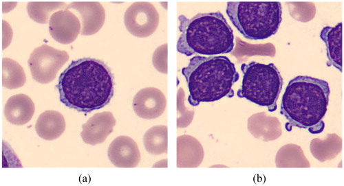
Figure 2. Lymphoma (a), blast (b), lymphocyte (c) and other cell (d).

Table 1. Total number of cells of each class in the dataset.

Class	Blast	Lymphoma	Lymphocyte	Others	Total
Number	465	696	486	26	1673

Methods

There are many object detection networks based on CNN, like R-CNN [15], Fast R-CNN [16], single shot multi-box detector (SSD) [17], and Faster R-CNN. Among these networks, Faster R-CNN has state-of-the-art performance, which won the 1st place in the COCO 2015 object detection competition. At the stage, the accuracy and robustness are important for a lymphoma diagnosis system, so we choose Faster R-CNN to achieve our goal.

Before we use the Faster R-CNN to detect whether there are lymphoma cells in the image and find their location, we need to train the network first. There are two ways to train a network. The first way is using a lot of images to train a random initialized network, which is called full training, and it will both cost a lot of time and computing resource. The other way is using a small dataset to fine-tune a pre-trained network, which is called transfer learning [18]. In our work, we choose the second way, because we do not have enough images to finish a full training. If we want to use our small dataset to achieve a full training, it is easy to overfit. Through fine-tuning, the pre-trained network can be fitted to our dataset.

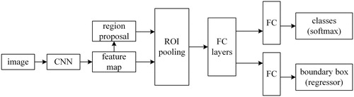
The weakness of Fast R-CNN is that it is difficult to find all the proposals of the input image, which makes it time-consuming while training the network and testing. Compared with Fast R-CNN, Faster R-CNN proposed Region Proposal Network (RPN), which would make it easy to predict the bounding boxes of an object. Faster R-CNN can be thought of as the combination of Fast R-CNN and RPN. The principle of Faster R-CNN is: the input image will be represented as a tensor, and the dimensionality of tensor depends on the dimension, width and height of the input image. Then the tensor will be sent into a pre-trained or initialized CNN to generate a feature map. After that, we will use region proposal network to calculate the feature to get a region proposal which may contain our target. And we use the region of interest pooling on the feature map to obtain a new tensor. Finally, the tensor will be put into the fully connected layers to classify the target and adjust the bounding box of the target. Figure 3 presents the architecture of Faster R-CNN.

Figure 3. Architecture of Faster R-CNN.

CNNs

Different CNNs have different ability in extracting features, so the classification result will be different. There are several CNNs integrated in Faster R-CNN. In our work, we chose three typical classification networks from them: ZF [19], VGG16 [20], and VGG_CNN_M_1024, to get a better classification result.

ZF: ZF is an eight-layer CNN, and its network structure is similar with that of AlexNet. But there are still two differences. The first difference is that the number of convolution kernel of the layer 3, layer 4, and layer 5 are changed; the other difference is that the size of the convolution kernel and stride of ZF are smaller than AlexNet. The convolution kernel size of ZF is 7 * 7, and that of AlexNet is 11 * 11. From the results in the paper, the classification results of ZF are better than those of AlexNet [19].

VGG16: VGG16 is a sixteen-layer CNN, and it has shown a good performance since it was proposed in 2014. It contains thirteen convolution layers and three fully connected layers, and after the second, the fourth, the seventh, the tenth and the last convolution layers, the network must have pooling respectively. Its convolution kernels are smaller than other networks; the size of most convolution kernels are 3 × 3; the rest are even 1 × 1. Although this network has many layers, it still can be trained fast.

VGG_CNN_M_1024: VGG_CNN_M_1024 is also an eight-layer CNN, and its frame is similar with ZF, which contains five convolution layers and three fully connected layers. The differences between them are that while convoluting, the ZF needs to pad the profile of an image but the VGG_CNN_M_1024 does not . Moreover the number of convolution kernels of the third, the fourth and fifth convolution layers are different.

Training methods

We used two training methods: End-to-end training method and 4-step alternating training method [14] to train the three convolutional neural networks respectively. For each training method, we use the same dataset and do not change the partition of the dataset.

End-to-end Training method: the End-to-end training method means that we only have to control the input data of the network, but pay no attention to the middle layers. Once the images are sent into the input layer of a network, we can get a predicted result from the output layer. The loss value was obtained by comparing the predicted result with the true result. The loss value can hardly be 0, and the loss will be back propagated to every layer of the network. And according to the loss, the weights of each layer are changed to make the model convergence.

4-Step Alternating Training method: Just as its name implies, there are 4 stages for the 4-Step Alternating Training method to train a model. The first step is using the pre-trained model to initialize and fine-tune the RPN and to generate the region proposal. The second step is sending the region proposals into an initialized classification network and training the classification network, and up to now, the PRN and the classification network have not shared the convolutional layers. The third step is re-initializing the RPN through the model obtained in the second step, but in this step, we should keep the shared convolutional layers fixed. The last step is using the RPN model obtained in the third step to re-initialize the classification network and using the region proposals to train it, but we just fine-tune the fully connected layers of the classification layers. In this way, we can keep the two networks sharing the same convolutional layers and combine the two networks to a united network.

Results and discussion

The pre-trained model we chose was pre-trained on the PASCAL Visual Object Classes Challenge 2007 (VOC2007), which is a large image dataset designed for object detection and segmentation. We divided our dataset into three parts like VOC2007, the training set (60%), the validation set (20%) and the testing set (20%), and they will be input to the network for training, validation and testing respectively. There are two types of images in our dataset: one target cell per image and multiple target cells per image. We divided the dataset randomly, so the training, validation, and testing set should contain both the two types of images in theory. In this way, we can reduce the influence of dataset as far as possible. Table 2 presents the number of images of each part.

Table 2. Number of images of each part.

	Training set	Validation set	Testing set	Total
Number	795	265	266	1326

During training, the training set is used to fit the model and the validation set is used to judge the learning status, adjust hyperparameters and select features. Those two parts of images will both influence the loss. The smaller the loss, the better the network fits the data. The Testing set is used to evaluate the trained model and get a mean Average Precision (mAP), which not only focuses on the object proposals but also on the object detection results [14]. The higher the mAP, the better the test result is.

The Faster R-CNN framework we used in this work was constructed on Caffe. In our experiment, the base learning rates are all 0.001 and will change after every 2000 trainings. With the help of graphic processing units, the training work can finish in an hour, and 266-images testing takes less than 3 min. While training the network through the End-to-end Training method, we fix the maximum iteration at 10000. While training through the 4-Step Alternating Training method, we fix the maximum iteration at 10000 for the RPN and the maximum iteration at 5000 for the classification network. Table 3 presents the mAP of the three networks trained through the two training methods.

Table 3. mAP of 6 combinations of different methods and networks.

Methods	Network	Lymphoma	Lymphocyte	Blast	Others	Mean mAP
4-Step Alternating Training	ZF	0.8657	0.8817	0.9007	0.5594	0.8019
	VGG16	0.8997	0.8990	0.9768	0.5455	0.8302
	VGG_CNN_M_1024	0.8953	0.9025	0.9974	0.8182	0.9033
End-to-end Training	ZF	0.9599	0.9659	0.9951	0.8239	0.9362
	VGG16	0.9544	0.9652	0.9900	0.7792	0.9222
	VGG_CNN_M_1024	0.9543	0.9677	0.9951	0.8242	0.9353

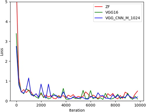
In our experiment, when using the 4-Step Alternating Training method, RPN is trained twice as often as the classification network, but compared with the End-to-end training method, the classification networks are trained the same number of times. From Table 3, we can find that the End-to-end Training method has a better performance than the 4-Step Alternating Training method. The reason is that our dataset is not large enough; overfitting may occur when using the 4-Step Alternating Training method. At the same time, the End-to-end Training method requires less computing resources and can be trained faster, because it does not need to train the RPN and the classification network respectively. So, the End-to-end Training method is a better choice. We can also find that the mAPs for each class in the three networks are almost similar. For the lymphoma, the mAPs of the three networks are all above 0.95; for the lymphocyte, the mAPs of the three networks are all above 0.96; and for the blast, the mAPs are even above 0.99. For other cells, the mAP is almost 0.82 for ZF and VGG_CNN_M_1024, but only 0.78 for VGG16. Because the number of other cells is smaller than other classes, and those cells do not have many common characteristics, this results in a decline in the classification performance. Figure 4 illustrates the loss for the three networks combined with the End-to-end Training method. We can observe that all the losses for the three networks fall down to 0.5 after training, which means that the three networks can converge well. We can also find that although the original loss for ZF is much bigger than the other two networks, its rate of convergence is faster. The original loss for VGG_CNN_M_1024 is the smallest among the three networks, but it must iterate more times to get convergence. So, we choose the VGG16 whose original loss is not very large and the VGG16 can get convergence after a few iterations to train the model for lymphoma diagnosis.

Figure 4. Loss for ZF (red), VGG16 (green), and VGG_CNN_M_1024 (blue).

Because our dataset is not very large, we decided to do a cross-validation to get a reliable result. We divided the dataset into five parts. One of them was fixed as the test set, and one of the remaining four was taken as the validation set, and the other three were used as the training set for a 4-fold cross-validation. The test mAPs are 0.9222, 0.9273, 0.9336 and 0.8943. We can find the results of cross-validation have no significant differences, which means our result is convincing.

As we have trained a model using VGG16 by the End-to-end Training method, we used some images of lymphoma, lymphocyte and blast which had not been sent into the network for training to run a test. During the test, if a cell is undetected or is categorized as others, we both classify it into the category of “others”. The test results are presented in Table 4. From Table 4, we can find that the detection rate of lymphoma is higher than 96%. Zorman et al. [21] used Symbol-Based Machine Learning Approach to Segment Follicular Lymphoma Images; they selected two decision trees: Decision tree with the highest accuracy on testing set and Decision tree with only one feature used. The overall accuracy of the first decision tree is 86.65% and the overall accuracy of the second decision tree is 83.63%. Spinosa et al. [22] used SVM to classify large B-cell lymphoma and the accuracy they obtained is nearly 92%. Compared to their test accuracies, our result is improved. In addition, they must complete image pre-processing and feature extraction before the training, and our method does not need it.

Table 4. Confusion matrix of the final model.

	Lymphoma	Lymphocyte	Blast	Others	Total
Lymphoma	74 (96.10%)	0 (0%)	0 (0%)	3 (3.90%)	77 (100%)
Lymphocyte	8 (2.93%)	259 (94.87%)	0 (0%)	6 (2.20%)	273 (100%)
Blast	23 (12.57%)	3 (1.64%)	130 (71.04%)	27 (14.75%)	183 (100%)

Note: For each grid, the table row presents the true class, and the table column presents the predicted class.

As the final model of Faster R-CNN which is trained using VGG16 and End-to-end training method achieved good results on the task of object detection, we wanted to find out how our dataset would perform on the task of object classification. We used our dataset for the training and testing of K-Nearest Neighbor (KNN) and VGG16. The test results of KNN and VGG16 are shown in Tables 5 and 6.

Table 5. Confusion matrix of KNN.

	Lymphoma	Lymphocyte	Blast	Total
Lymphoma	15 (40.54%)	5 (13.51%)	17 (45.95%)	37 (100%)
Lymphocyte	17 (40.48%)	6 (14.29%)	19 (45.24%)	42 (100%)
Blast	14 (38.89%)	3 (8.33%)	19 (52.78%)	36 (100%)

Table 5 is the confusion matrix of KNN. KNN is a classification method that depends on the distance of images. Because the background of blood cell images is similar, KNN can get a satisfactory result in theory. But from Table 5, we can find the test results are not satisfactory, because these cells are not very different in morphology. This is why it is difficult for doctors to distinguish them. In our work, we use about 200 images of each class for training, about 40 images of each class for testing, and every image only contains one cell; in this way, we can reduce the influence of the background as far as possible.

Table 6 is the confusion matrix of VGG16. We trained and tested VGG 16 with the same dataset as Faster R-CNN. Unlike Faster R-CNN, VGG 16 is tested in units of images, whereas Faster R-CNN is tested in units of cells. Although the total numbers in Tables 4 and 6 are different, they are actually the same dataset because some images contain multiple cells. From Table 6, we can find that although the detection rate of lymphoma is as high as 95%, the false detection rate is also quite high.

Table 6. Confusion matrix of VGG16.

	Lymphoma	Lymphocyte	Blast	Total
Lymphoma	38 (95%)	1 (2.5%)	1 (2.5%)	40 (100%)
Lymphocyte	82 (30.83%)	184 (69.17%)	0 (0%)	266 (100%)
Blast	26 (17.22%)	1 (0.66%)	124 (82.12%)	151 (100%)

Comparing Tables 4–6, we find that Faster R-CNN has higher detection rate and lower false detection rate than the other two methods. Although the results of Faster R-CNN are not perfect(for example, blast has a higher probability of being misclassified as lymphoma), it can be used as an auxiliary method to help doctors diagnose lymphoma faster.

Nowadays, there are fewer experiments using only image processing methods to detect lymphoma cells, and most experiments are based on biological information, which is very time-consuming and labor-intensive. With the development of deep learning, it is a general trend to combine CNN and medical images, and we can reduce the workload of doctors and help them get test results faster.

The accuracy of a model is largely related to the training data, so obtaining more training data and expanding our dataset through methods such as data augmentation are our future work. In addition, continuing to fine-tune the model is also an important work to improve the detection rate of lymphoma. We hope that our network can be used in real life to help doctors detect lymphoma faster and more accurately with our efforts.

Conclusions

In this paper, we built a high-quanlity blood cell dataset that mainly contains lymphoma cells, lymphocyte cells, blast cells and an annotation file of each image file. The dataset can be helpful to the development of deep learning in this field. In order to realize the automatic detection of lymphoma cells and find their location on the image, we combined the images and annotation files from our dataset with Faster R-CNN to fine-tune a pre-trained model. We determined the final model by testing the performance of the combination of different training methods and networks on this dataset and tested its performance with a brand new dataset. From the final test result, we find that the detection rate of lymphoma is higher than 96%.

Data availability statement

Raw data were generated at East China Normal University. Derived data supporting the findings of this study are available from the corresponding author Qingli Li on request. More details can be found from http://bio-hsi.ecnu.edu.cn

Disclosure statement

No potential conflict of interest was reported by the author(s).

Additional information

Funding

This work was supported by the National Natural Science Foundation of China (Grant No. 61975056, 61901173), the Shanghai Natural Science Foundation (Grant No. 19ZR1416000), the Science and Technology Commission of Shanghai Municipality (Grant No. 14DZ2260800, 18511102500).

References

- Siegel RL, Miller KD, Jemal A. Cancer statistics, 2017. CA Cancer J Clin. 2017; 67(1):7–30.
- Barbe E, de Boer M, de Jong D. A practical cytological approach to the diagnosis of breast-implant associated anaplastic large cell lymphoma. Cytopathology. 2019;30(4):363–369.
- Willemze R, Cerroni L, Kempf W, et al. The 2018 update of the WHO-EORTC classification for primary cutaneous lymphomas. Blood. 2019;133(16):1703–1714.
- Garg A, Hosfield EM, Brickner L. Disseminated intravascular large B cell lymphoma with slowly decreasing high-density lipoprotein cholesterol. South Med J. 2011;104(1):53–56.
- Montes-Mojarro I-A, Bonzheim I, Quintanilla-Martínez L, et al. Molecular diagnosis of lymphoma: a case-based practical approach. Diagn Histopathol. 2019;25(6):229–239.
- Howell DA, Hart RI, Smith AG, et al. Disease-related factors affecting timely lymphoma diagnosis: a qualitative study exploring patient experiences. Br J Gen Pract. 2019; 69(679) :e134–e145.
- Robertson S, Azizpour H, Smith K, et al. Digital image analysis in breast pathology-from image processing techniques to artificial intelligence. Transl Res. 2018; 194:19–35.
- Mohan G, Subashini MM. MRI based medical image analysis: Survey on brain tumor grade classification. Biomed Signal Process Control. 2018; 39:139–161.
- Razzak MI, Naz S, Zaib A. Deep learning for medical image processing: Overview, challenges and the future. In Classification in BioApps. 2018. Cham, Switzerland: Springer. p. 323–350.
- Habibzadeh M, et al. Automatic white blood cell classification using pre-trained deep learning models: ResNet and Inception. Tenth International Conference on Machine Vision (ICMV 2017), 2018. Bellingham, USA. International Society for Optics and Photonics. 1069612.
- Tiwari P, Qian J, Li Q, et al. Detection of subtype blood cells using deep learning. Cognit Syst Res. 2018; 52:1036–1044.
- Sahlol AT, Kollmannsberger P, Ewees AA. Efficient classification of white blood cell leukemia with improved Swarm optimization of deep features. Sci Rep. 2020; 10(1) :2536
- Rehman A, Abbas N, Saba T, et al. Classification of acute lymphoblastic leukemia using deep learning. Microsc Res Tech. 2018; 81(11) :1310–1317.
- Ren S, He K, Girshick R, et al. Faster R-CNN: Towards Real-Time Object Detection with Region Proposal Networks. IEEE Trans Pattern Anal Mach Intell. 2017; 39(6) :1137–1149.
- Girshick R, et al. Rich feature hierarchies for accurate object detection and semantic segmentation. Proceedings of the IEEE conference on computer vision and pattern recognition, Columbus, OH, USA. 2014. 580–587
- Girshick R. Fast r-cnn. Proceedings of the IEEE international conference on computer vision, Santiago, Chile. 2015, p. 1440–1448.
- Liu W, et alSsd. Single shot multibox detector. In Leibe B, Matas J, Sebe N, Welling M, editors. European conference on computer vision, Amsterdam, Netherlands. 2016. Springer. 21–37.
- Tajbakhsh N, et al. Convolutional neural networks for medical image analysis: Full training or fine tuning?. IEEE Trans Med Imag. 2016; 35(5) :1299–1312.
- Zeiler MD, Fergus R. Visualizing and understanding convolutional networks. in European conference on computer vision. 2014. Springer.818–833
- Simonyan K, Zisserman A. Very deep convolutional networks for large-scale image recognition. 3rd International Conference on Learning Representations, ICLR 2015, 2015. San Diego, CA, United states: International Conference on Learning Representations, ICLR; 2015. 1–14
- Zorman M, et al. Symbol-based machine learning approach for supervised segmentation of follicular lymphoma images. In Kokol P, Podgorelec V, MiceticTurk D, Zorman M, Verlic M, editors. Twentieth IEEE International Symposium on Computer-Based Medical Systems (CBMS’07). 2007. Los Alamitos, CA, USA. IEEE Computer Soc.115–120.
- Spinosa EJ, de Leon Ferreira ACP. SVMs for novel class detection in Bioinformatics. WOB, Brasília, Distrito Federal, Brazil. 2004. 2004, p. 81–88.