An efficient protein homology detection approach based on seq2seq model and ranking

Abstract

Evolutionary information is essential for the protein annotation. The number of homologs of a protein retrieved is correlated with the annotations related to the protein structure or function. With the continuous increase in the number of available sequences, fast and effective homology detection methods are particularly important. To increase the efficiency of homology detection, a novel method named CONVERT is proposed in this paper. This method regards homology detection as a translation task and presents a concept of representative protein. Representative proteins are not real proteins. A representative protein corresponds to a protein family, it contains the characteristics of the family. Our method employs the seq2seq model to establish the many-to-one relationship between proteins and representative proteins. Based on the many-to-one relationship, CONVERT converts protein sequences into fixed-length numerical representations, so as to increase the efficiency of homology detection by using numerical comparison instead of sequence alignment. For alignment results, our method adopts ranking to obtain a sorted list. We evaluate the proposed method on two benchmark datasets. The experimental results show that the performances of our method are comparable with the state-of-the-art methods. Meanwhile, our method is ultra-fast and can obtain results in hundreds of milliseconds.

Keywords:

• Homology detection
• translation task
• seq2seq model
• ranking

Introduction

With the rapid development of next-generation sequencing technology, the number of biological sequence data is increasing explosively. By September 2020, more than 180 million protein sequences in TrEMBL [1] have been identified, and more than 99% of them are still waiting for annotation. How to analyze these sequences effectively has become an important issue in the field of bioinformatics. Homology detection plays a crucial role in protein sequence analysis because of its role in protein structure [2] and function [3, 4].

Homology detection developed rapidly, and many methods have been proposed. The early methods are based on pairwise sequence alignment [5, 6]. A query is aligned one by one with the artificially labelled protein sequences in a dataset, and the homology of the query is calculated based on the scores of alignment results. With the increase in the number of protein structures measured, the time overhead of the pairwise sequence alignment methods is also increasing. To improve the alignment speed, BLAST [7] and FASTA [8] were proposed. These two methods make a compromise with part of the accuracy to get faster alignment speed. However, the pairwise sequence alignment algorithms cannot accurately detect the homology between sequences with low similarity. So homology detection methods based on protein sequence profile were proposed, such as PL-search [9], PSI-BLAST [10], SMI-BLAST [11], COMA [12], Phyre [13] and FFAS [14]. These methods adopt multi-sequence alignment to generate a position specific scoring matrix of a query to assist detection. Since these methods take into account the evolutionary information of proteins, the sensitivity of recognition is greatly improved. Later, some researchers employed hidden Markov model for homology detection [15–17]. They established a corresponding hidden Markov model for each protein in the database, and determined the sequence homology by comparing the hidden Markov models. With the increasing popularity of machine learning, researchers began to try to apply machine learning algorithms [18–21] to homology detection, treating homology detection as a multi-classification task. But almost all discriminant methods need appropriate length of eigenvectors as input, and the quality of eigenvectors directly determines the effectiveness of such methods [22]. Therefore, how to generate appropriate eigenvectors has always been the focus of discriminant methods. Different from the discriminant methods, ranking methods [23–25] regard the homology detection as a ranking task. For a query sequence, ranking methods calculate a sorted list according to the evolutionary similarity.

Evolutionary information is essential for homology detection. However, the calculation of evolutionary information depends on traditional sequence alignment algorithms or their improved algorithms. This means that the shortcomings of traditional sequence alignment algorithms will affect the effect of other methods which are based on the evolutionary information. Therefore, how to utilize only protein sequence information for homology detection is still crucial for protein sequence analysis. Meanwhile, massive amounts of protein sequence data urgently need fast and reliable homology detection methods.

In this study, we propose a novel method called CONVERT for homology detection. The proposed method regards homology detection as a translation task which combines the seq2seq model and ranking. Firstly, each family’s representative protein is generated based on semi-global alignment. Secondly, the many-to-one relationship between proteins and representative proteins is established based on the seq2seq model. Thirdly, the decoder is discarded, and the encoder part is retained to generate eigenvectors of proteins. Finally, a sorted list is calculated for the query sequence based on the eigenvectors. The proposed method provides a unified model for all families, and transforms the sequence data into fixed-length numerical data which is easier to calculate.

Materials and methods

Representation of sequence

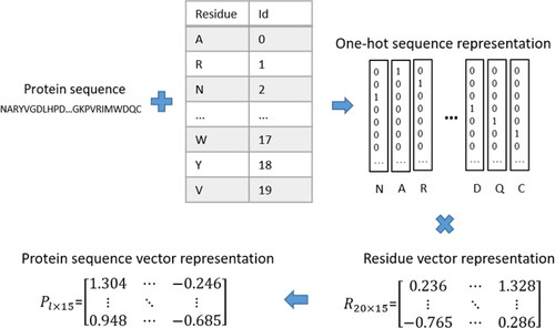
For neural networks, the alphabetical representation of amino acid residues cannot be utilized as input, so we need to convert alphabetical representation into numeric representation. One-hot encoding is usually utilized to encode protein sequences. However, one-hot encoding cannot reflect the relationship between residues. So we adopt word embedding [26, 27] to encode sequences to capture the relationship between residues. The word embedding process is shown in Figure 1. To retain abundant information of protein sequences, we embed residues into 15-dimensional space. The numeric representation of residues will be updated throughout the training process, and the relationship between residues will become mature through repeated training.

Figure 1. The process of word embedding. l denotes the length of protein sequence. The purpose of word embedding is to get an appropriate R, which can reflect the relationship among residues.

Semi-global alignment

Needleman-Wunsch [5] is a basic algorithm in protein sequence analysis. It is a global alignment algorithm, and its basic idea can be briefly described as: using the iterative method to calculate the similar scores of two sequences, and storing similar scores in a score matrix, then an optimal comparison result is found by dynamic programming based on the matrix. Needleman-Wunsch can find the optimal comparison result when comparison sequence lengths are similar. In general, the sequence lengths in the same family are similar, but not absolute. Therefore, we choose the semi-global alignment [28] as the basic alignment algorithm in this work. The formula of semi-global alignment is as follows: (1) $$F\left(i,\mathrm{ }0\right)=0\mathrm{ }or\mathrm{ }F\left(0,j\right)=0$$(1) (2) $$F\left(i,j\right)=\mathit{max}\{\begin{array}{c}F\left(i-1,j-1\right)+s(x_i,y_j)\\ F\left(i-1,j\right)+d \\ F\left(i,j-1\right)+d \end{array}$$(2) where s(x_i, y_j) is the score in the scoring matrix when x_i is aligned with y_j, d is the penalty for the gap. Formula (2) is the formula of Needleman-Wunsch, and Formula (1) and (2) make up the formula of semi-global alignment. Formula (1) initializes the first row or column corresponding to the long sequence to zero, so that implementing no penalty for front-end vacancies in long sequence. In backtracking, the first step is to backtrack from the lower right corner to the maximum number in row or column corresponding to the long sequence. Then, like the Needleman-Wunsch, it backtracks to the upper left corner of the matrix. When alignment sequence lengths are similar, the results of semi-global alignment and Needleman-Wunsch are similar. When alignment sequence lengths are quite different, the result of semi-global alignment tends to embed the short sequence into the long sequence.

Bidirectional GRU

Recurrent Neural Network (RNN) [29, 30] is a key technology in time-series data processing [31, 32]. Gated Recurrent Unit (GRU) [33], as a variant of RNN, has the advantages of simplicity and effectiveness. It is a very popular RNN nowadays.

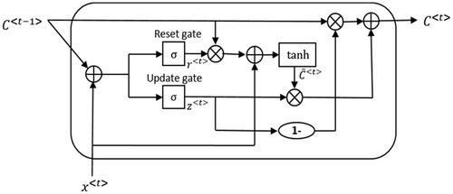
The cell structure of GRU is shown in Figure 2. It has two gates, the update gate and the reset gate. The update gate helps the model to determine how much of the past information needs to be passed along to the future. The reset gate is used from the model to decide how much of the past information to forget.

Figure 2. The cell structure of GRU. C^{<t -1>} denotes the state of the previous time of t, x^<t> is the input of the time t, C^<t> is the state of time t. σ and tanh are the activation function. The state of time t depends not only on the input of the current time, but also on the inputs of the previous times.

In unidirectional RNN, the transmission between states is a one-way process. The state of time t can only be obtained from the past sequence x₀, x₁, $\cdots ,$ x_(t-1) and x_t. For the residues in protein sequences, they depend not only on the sequence on the left, but also on the sequence on the right. To obtain positive and negative direction dependency information of residues, we utilize bidirectional GRU as the encoder of seq2seq model.

CONVERT

1. Generate representative protein: Generating representative proteins involves two phases: select benchmark protein and generate representative protein. When the length difference between the longest and shortest sequences is less than 20 residues in a family, we choose the shortest sequence as the benchmark protein. Otherwise, we randomly select a sequence whose length is between (m+(l-m)/4) and (l-(l-m)/4) as the benchmark protein, where m is the average length and l is the longest length of sequences in the family. Such selection can effectively avoid situations in which the longest or shortest sequence is a special case. After selecting the benchmark proteins, the next phase is to generate representative proteins. We utilize a semi-global alignment algorithm based on BLOSUM62 to align all sequences with their benchmark proteins. The gaps in the alignment results of the benchmark proteins are treated as the increases of other sequences, and deleted. As shown in Figure 3, there are two sequences stlye and slfeql, and the alignment results are stlye– and s-lfeql. If stlye is the benchmark protein, the final result of slfeql is s-lfe. If slfeql is the benchmark protein, the final result of stlye is slye–. Thus, the final results in a family have the same sequence length (the length of the benchmark protein). Then, the residues with the highest frequency in the same position in the results of the same family are selected and spliced into the representative protein of this family.

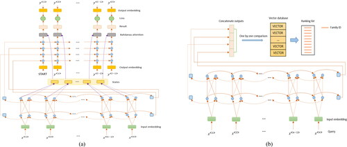
2. Establish relationship: The seq2seq model [34, 35] is widely used in question answering system and machine translation. The process of its operation is: encoder transforms a sequence into a fixed-length context vector, and a decoder transforms the context vector into a target sequence. For a general seq2seq model, no matter which residue in the output is generated, any residue in the input sequence has the same influence on that residue. When the length of the input sequence is short, the effect on the result is small. Unfortunately, protein sequences are usually long. According to the generation process of the representative protein, for a residue x in a representative protein, the residues in the aligned sequences whose positions are similar to x have greater influence on x’s generation. Therefore, we utilize the Bahdanau Attention [36], which makes neuro-machine translation focus on some important parts while ignoring others, to highlight the importance of residue location information. As shown in Figure 4(a), we utilize bidirectional GRU with two hidden layers as the encoder and GRU with four hidden layers as the decoder. The protein sequences are used as the input, and the corresponding representative proteins are used as the output to train the model.

3. Detect homology: After the seq2seq model training, we convert all sequences in a database into numerical representations using the trained encoder. All the numerical representations make up the vector database. As shown in Figure 4(b), when a query sequence comes in, it is put into the encoder for coding, and the coding result is compared with the vectors in the vector database. We use Euclidean distance to measure the distance between vectors. The smaller the distance between two vectors, the more the corresponding two sequences tend to be homologous. For the comparison results, we adopt the idea of ranking methods to sort them. As the number of proteins is very large, it is extremely expensive in terms of time to sort all the results. However, there is no need to sort all results, we just sort the top-k. The value of k can be specified as required. Moreover, the results generated by our method can provide remote homology information. As we know, the similarity between proteins belonging to the same superfamily but different families is low, so to produce representative proteins for different superfamilies is not a good choice. Fortunately, the IDs of the proteins in the dataset can provide rich information like fold, superfamiliy, family. As shown in Figure 4(b), the ranking list consists of family IDs. When we obtain the ranking list of a query, we can obtain superfamily information and even fold information of the query in addition to family information.

Figure 3. The processing of alignment results. The residues corresponding to the gaps in the alignment results of the benchmark protein will be deleted.

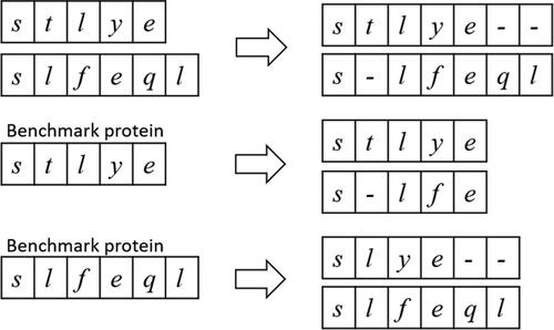
Figure 4. Architecture of CONVERT in the training phase (a) and the testing phase (b). The left figure shows the architecture of CONVERT in the training phase. Encoder is composed of bidirectional GRU with two hidden layers, and decoder is composed of GRU with four hidden layers. Firstly, the word embedding is used to generate the numeric representation of the training samples. Secondly, encoder generates the context vectors of the training samples. Thirdly, decoder generates the results according to the intermediate states and the context vector. Finally, the loss is calculated and the parameters are updated. The right figure shows the architecture of the testing phase of CONVERT. A query sequence is put into the encoder for coding, and the coding result is compared with the vector database to obtain the top-k of the result as required.

Dataset, preprocessing and validation

1. Dataset: In this work, we adopt SCOP (version 1.75) [37] and SCOPe (version 2.06) [38] to evaluate the performance of our method. SCOP benchmark dataset contains 16712 amino acid sequences from 3901 families. And SCOPe contains 30201 amino acid sequences from 4850 families. All data can be downloaded from http://SCOP.berkeley.edu/astral/.

2. Preprocessing: For each family in the experimental data, we randomly select a sequence to join the testing data and the rest to join the training data. However, the training data is severely unbalanced. Some families contain hundreds of protein sequences, while some families contain only a few. To avoid the adverse effect of unbalanced data on model training, we utilize the oversampling on the training set: assuming n is the number of proteins in the family with the most proteins in the training set, for a family with fewer proteins than n, we repeatedly select sequences from this family randomly and add them to the training set until the number of proteins in this family equals n. Finally, the data preprocessing before the model training is completed by shuffling the training set.

3. Measurements: On the SCOP dataset, the performance of CONVERT compared with other methods is evaluated by the area under the ROC curve (AUC) and the AUC score evaluated on the first 1000 false positives (AUC1000), which are the same metrics used in [39]. Since we just sort top-k results for a query sequence, the Precision in Top-k (PIT-k) (PIT-1, PIT-2, PIT-3 stand for k equals to 1,2,3, respectively) is used to evaluate the performance of CONVERT with different k on the SCOP and SCOPe datasets. For a query sequence q, if the top-k results contain a sequence from the same family as q, the recall is successful. We assume there are m query sequences, of which l query sequences are recalled successfully, the PIT-k is defined as $\frac{l}{m}.$

Results

Comparison with state-of-the-art methods

In this study, we selected some of the most commonly used homology detection algorithms and compared them with CONVERT on SCOP. The AUC and AUC1000 scores of PHMMER [40], CSBLAST [41], HHSEARCH [17], NCBI-BLAST [42], USEARCH [43], FASTA [8], UBLAST [43], reported in Table 1, were extracted from [39], in which the authors provided a detailed benchmark of these methods.

Table 1. Comparison of CONVERT performance on the SCOP dataset

Method	AUC	AUC1000
PHMMER	0.959	0.903
CSBLAST	0.961	0.899
HHSEARCH	0.951	0.877
NCBI-BLAST	0.937	0.857
USEARCH	0.938	0.853
FASTA	0.919	0.834
UBLAST	0.842	0.785
CONVERT	0.931	0.856

As shown in Table 1, the AUC of CONVERT is 0.028 lower than PHMMER, 0.03 lower than CSBLAST and 0.012 better than FASTA, 0.089 better than UBLAST. In terms of AUC1000, CONVERT is comparable to NCBI-BLAST, which is ranked fourth. Overall, PHMMER, CSBLAST and HHSEARCH are the most reliable homology detection methods. And CONVERT is comparable to methods such as NCBI-BLAST and USEARCH. Although the scores are different for each method, we can intuitively see from Figure 5 that, except for UBLAST, the overall quality of the other methods is similar.

Figure 5. Comparisons among different methods on the SCOP dataset in terms of AUC and AUC1000.

The dependence on the value of k

In order to know how different values of k influence the PIT-k, we chose ten different numbers as the values of k, namely 1, 2, 3, 5, 7, 10, 15, 20, 25, 30. The detailed results are shown in Table 2 and Table 3. The growth trend of PIT-k with the increase of k is shown in Figure 6, from which we can obviously see the following: (1) As the value of k increases, so does the precision. But if the value of k is too large, TIP-k will be meaningless. We need to choose the appropriate k to ensure the accuracy of homology detection while keeping the detection time low. (2) When k equals 15, the accuracy is 0.922 on the SCOP benchmark dataset and 0.933 on the SCOPe benchmark dataset, and when the value of k is greater than 15, the accuracy has risen slowly, indicating that 15 is a good choice for k, but any k may be used.

Figure 6. The growth trend of TIP-k with the increase in k value.

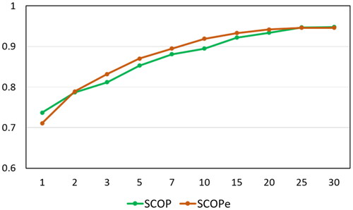
Table 2. The performance of CONVERT with different k on the SCOP dataset.

Method	k	PIT-k
CONVERT	1	0.737
CONVERT	2	0.787
CONVERT	3	0.812
CONVERT	5	0.853
CONVERT	7	0.881
CONVERT	10	0.895
CONVERT	15	0.922
CONVERT	20	0.934
CONVERT	25	0.947
CONVERT	30	0.948

Table 3. The performance of CONVERT with different k on the SCOPe dataset.

Method	k	PIT-k
CONVERT	1	0.711
CONVERT	2	0.789
CONVERT	3	0.832
CONVERT	5	0.870
CONVERT	7	0.895
CONVERT	10	0.919
CONVERT	15	0.933
CONVERT	20	0.942
CONVERT	25	0.946
CONVERT	30	0.946

CONVERT has linear complexity

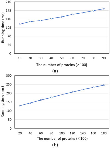
We tested the testing sets of SCOP and SCOPe on a PC with CPU i7-6700 and RAM 8 G. And we transformed protein sequences into 1200 D vectors, and sorted the top-100 of the results. As the lengths of the sequences are different, we used the average running time to evaluate the efficiency of CONVERT. We generated nine datasets with different sizes for the two datasets (ranging from 1000 to 9000 for SCOP, and ranging from 2000 to 18000 for SCOPe). In Figure 7, we can see that the two graphs are similar: as the number of proteins in the database increases, the running time increases linearly and slowly. If we extend the line in Figure 7(a) or Figure 7(b) to the left, it will not intersect the coordinate axis at (0, 0), but at approximately (0, 100). That is, on average, it takes about 100 milliseconds for CONVERT to convert a sequence into a vector. Assuming that the time required for the CONVERT transformation sequence is t₁, the time required for the comparison of two vectors is t₂, and the database size is n, the time complexity of CONVERT is O(t₁+n×t₂), where t₁ and t₂ are constants.

Figure 7. Growth of CONVERT's runtimes with increasingly large dataset size on SCOP (a) and SCOPe (b). Plot empirically showing that as the number of proteins in the database increases, the running time of CONVERT increases linearly and slowly.

Discussion

Representative protein is a key in CONVERT

The representative protein is formed in a manner similar to multi-sequence alignment. A representative protein of a family extracts the commonness of the proteins in the family, so it can represent this family objectively and comprehensively. With characterizing proteins, we can establish many-to-one relationships between proteins and representative proteins. So CONVERT can skilfully transform a multi-classification task into a translation task, bypassing the shortcomings of multi-classification models that are difficult to achieve satisfactory accuracy when facing thousands of categories.

Considerations on the feasibility

The 5-fold cross-validation was used in our experiment. That is, one protein is randomly selected from each family to construct the testing set, and the rest are used as training data, repeated five times, and the average result is the final result. Although the experimental results still have some randomness, it is undeniable that the credibility is still high. From Figure 7, we can roughly calculate that for every 1000 increase in the size of the database, the running time of CONVERT, which sorts the top-100 of the results, will increase by about 10 millisecondsons. This means that for databases with size less than 100000, CONVERT can get results in one second. From Tables 2 and 3, we can see that when k is 20, the accuracy of CONVERT on the two data sets exceeds 93%. The 5-fold cross-validation ensures the reliability of the experiment, and the experiment results show that our proposed method works well. Therefore, it is anticipated that CONVERT will become a very useful computational tool for sequence analysis.

CONVERT can reduce the detection time

Instead of generating a model for each family, CONVERT generates one model for all families. On the surface, going from multiple models to one can save a lot of time, but it does not. Firstly, when a single model can replace multiple models, this means that the single model is much more complex. Secondly, CONVERT will spend a lot of time to convert the protein database to the vector database. Of course, that time has to been spent, but not every time a query sequence is detected. After CONVERT training, all vectors are generated only once. When a new sequence needs to be detected, it only takes the time required of the CONVERT to transform the sequence to the corresponding vector and the time of the vector comparison. Therefore, CONVERT can quickly select a few families out of thousands for priority detection.

Conclusions

In this paper, we proposed a novel homology detection method which treats the homology detection as a translation task. Our method greatly reduces the time required for homology detection. Meanwhile, as the amount of data increases, the time spent on our proposed method increases linearly. Our method no longer focuses on whether two proteins are homologous, but adopts the idea of the ranking method to sort the results. Therefore, our method can help researchers quickly select useful sequences from the database, greatly reducing the cost of scientific research.

Disclosure statement

No potential conflict of interest was reported by the author(s).

Data availability statement

All data that support the findings in this study can be accessed at https://github.com/Gaoyitu/CONVERT. Data are available from the corresponding author upon reasonable request.

Additional information

Funding

This study is supported by the National Natural Science Foundation of China (No. 61863036) and the Yunnan University's Research Innovation Fund of Graduate Students (No. 2020296). We thank to the support of Scientific Research Fund of Education Department of Yunnan Province (No. 2017YJS108) and Doctoral Candidate Academic Award of Yunnan Province.

References

- Bateman A, Martin MJ, O'Donovan C, et al. UniProt: a hub for protein information. Nucleic Acids Res. 2015;43(D1):D204–D212.
- Popov I. S-motifs as a new approach to secondary structure prediction: comparison with state of the art methods. Biotechnol Biotechnol Equipment. 2012;26(3):3016–3020.
- Radivojac P, Clark WT, R. Oron T, et al. A large-scale evaluation of computational protein function prediction. Nat Methods. 2013;10(3):221–227.
- Liu L, Tang L, He LB, et al. Predicting protein function via multi-label supervised topic model on gene ontology. Biotechnology & Biotechnological Equipment. 2017;31(3):630–638.,
- Needleman SB, Wunsch CD. A general method applicable to the search for similarities in the amino acid sequence of two proteins. J Mol Biol. 1970;48(3):443–453.
- Smith TF, Waterman MS. Identification of common molecular subsequences. J Mol Biol. 1981;147(1):195–197.
- Altschul SF, Gish W, Miller W, et al. Basic local alignment search tool. J Mol Biol. 1990;215(3):403–410.
- W. R P. Rapid and sensitive sequence comparison with FASTP and FASTA. Meth Enzym. 1990;183:63–98.
- Jin X, Liao Q, Liu B. PL-search: a profile-link-based search method for protein remote homology detection. Brief Bioinformatics. 2020;,
- Altschul SF, Madden TL, Schaffer AA, et al. Gapped BLAST and PSI-BLAST: a new generation of protein database search programs. Nucleic Acids Res. 1997;25(17):3389–3402.,
- Jin X, Liao Q, Wei H, et al. SMI-BLAST: a novel supervised search framework based on PSI-BLAST for protein remote homology detection. Bioinformatics. 2020;
- Margelevicius M, Laganeckas M, Venclovas C. COMA server for protein distant homology search. Bioinformatics. 2010;26(15):1905–1906.
- Kelley LA, Sternberg MJE. Protein structure prediction on the web: a case study using the Phyre server. Nat Protoc. 2009;4(3):363–371.
- Jaroszewski L, Li ZW, Cai XH, et al. FFAS server: novel features and applications. Nucleic Acids Res. 2011;39(Web Server issue):W38–W44.,
- Mistry J, Finn RD, R. Eddy S, et al. Challenges in homology search: HMMER3 and convergent evolution of coiled-coil regions. Nucleic Acids Res. 2013;41(12)
- Remmert M, Biegert A, Hauser A, et al. HHblits: lightning-fast iterative protein sequence searching by HMM-HMM alignment. Nat Methods. 2011;9(2):173–175.,
- Soding J. Protein homology detection by HMM-HMM comparison. Bioinformatics. 2005;21(7):951–960.
- Liu B, Li SM. ProtDet-CCH: Protein Remote Homology Detection by Combining Long Short-Term Memory and Ranking Methods. IEEE/ACM Trans Comput Biol Bioinform. 2019;16(4):1203–1210.
- Liu B, Zhang DY, Xu RF, et al. Combining evolutionary information extracted from frequency profiles with sequence-based kernels for protein remote homology detection. Bioinformatics. 2014;30(4):472–479.,
- Zhao XW, Zou Q, Liu B, et al. Exploratory predicting protein folding model with random forest and hybrid features. CP. 2015;11(4):289–299.
- Guo Y, Yan K, Wu H, et al. ReFold-MAP: Protein remote homology detection and fold recognition based on features extracted from profiles. Anal Biochem. 2020;611:114013.,
- Raimondi D, Orlando G, Moreau Y, et al. Ultra-fast global homology detection with discrete cosine transform and dynamic time warping. Bioinformatics. 2018;34(18):3118–3125.,
- Chen JJ, Guo MY, Wang XL, et al. A comprehensive review and comparison of different computational methods for protein remote homology detection. Brief Bioinform. 2018;19(2):231–244.,
- Jung I, Kim D. SIMPRO: simple protein homology detection method by using indirect signals. Bioinformatics. 2009;25(6):729–735.
- Melvin L, Weston J, Leslie C, et al. RANKPROP: a web server for protein remote homology detection. Bioinformatics. 2009;25(1):121–122.,
- Mikolov T, Quoc VL, Llya S. Exploiting similarities among languages for machine translation. axXiv, 1309.4168, 2013
- Lai SM, Liu K, He SZ, et al. How to generate a good word embedding. IEEE Intell Syst. 2016;31(6):5–14.,
- Suzuki H, Kasahara M. Introducing difference recurrence relations for faster semi-global alignment of long sequences. BMC Bioinf. 2018;19(S1)
- Hochreiter S, Schmidhuber J. Long short-term memory. Neural Comput. 1997;9(8):1735–1780.
- Rodriguez P, Wiles J, Elman JL. A recurrent neural network that learns to count. Conn. Sci. 1999;11(1):5–40.
- Chang XJ, Ma ZG, Lin M, et al. Feature Interaction Augmented Sparse Learning for Fast Kinect Motion Detection. IEEE Trans on Image Process. 2017;26(8):3911–3920.,
- Hirschberg J, Manning CD. Advances in natural language processing. Science. 2015;349(6245):261–266.
- Cho K, Merrienboer BV, Gulcehre C, et al. Learning phrase representations using RNN encoder-decoder for statistical machine translation. arXiv, 1406.1078, 2014
- Baltrusaitis T, Ahuja C, Morency LP. Multimodal machine learning: a survey and taxonomy. IEEE Trans Pattern Anal Mach Intell. 2019;41(2):423–443.
- Sutskever I, Vinyals O, Le QV. Sequence to sequence learning with neural work. In 28th Conference on Neural Information Processing Systems. 2014;27:3104–3112.
- Bahdanau D, Cho K, Bengio Y. Neural machine translation by jointly learning to align and translate. arXiv, 1409.0473, 2014;
- Andreeva A, Howorth D, Chandonia JM, et al. Data growth and its impact on the SCOP database: new developments. Nucleic Acids Res. 2008;36(Database issue):D419–D425.,
- Chandonia JM, Fox NK, Brenner SE. SCOPe: manual curation and artifact removal in the structural classification of proteins - extended Database. J Mol Biol. 2017;429(3):348–355.
- Saripella GV, Sonnhammer ELL, Forslund K. Benchmarking the next generation of homology inference tools. Bioinformatics. 2016;32(17):2636–2641.
- Finn RD, Clements J, Eddy SR. HMMER web server: interactive sequence similarity searching. Nucleic Acids Res. 2011;39(Web Server issue):W29–W37.
- Biegert A, Soding J. Sequence context-specific profiles for homology searching. Proc Natl Acad Sci U S A. 2009;106(10):3770–3775.
- Boratyn GM, Camacho C, Cooper PS, et al. BLAST: a more efficient report with usability improvements. Nucleic Acids Res. 2013;41(Web Server issue):W29–W33.
- Edgar RC, Notes A. Search and clustering orders of magnitude faster than BLAST. Bioinformatics. 2010;26(19):2460–2461.