Research on prediction of contact stress of acetabular lining based on principal component analysis and support vector regression

Abstract

In the "worst-case" selection of hip prosthesis wear, it is necessary to calculate the contact stress of the acetabular liner. However, there are various combinations of acetabular prostheses. If calculated one by one, it will cause a large workload, a repeated and tedious calculation problem. To solve this problem, a machine learning prediction method by combining principal component analysis and support vector regressions (PCA-SVR) was established. First, the finite element method is used to analyze and calculate the contact stress of the acetabular liner in a typical combination to form a basic data set with the key size of the acetabular prosthesis as input and the contact stress as output; then, based on this data set, the PCA reduces the dimension of the input to obtain a new data set. Finally, based on this data set, SVR is used to establish the mapping model, and the optimal value of the model parameter C and $\gamma$ is obtained by combining K-fold cross-validation and grid search method. The maximum absolute error of the prediction on the test data set is only 0.1986, the root mean square error RMSE is only 0.09309, and the R² value is 0.9426, which verifies the effectiveness of the prediction model. At the same time, the prediction performance is compared with the Ridge regression and Lasso models, which further verifies the superiority of the proposed method.

Keywords:

• Worst-case
• acetabular prosthesis
• PCA-SVR
• contact stress
• prediction model

Introduction

Artificial hip replacement has achieved great success in treating bone diseases such as hip fractures, congenital acetabular dysplasia, and femoral head necrosis. Contact stress is an important part of biomechanics, which has been the focus of research on biomechanics scholars since the birth of artificial joints. Maxian et al. [1] established a three-dimensional non-linear contact finite element method for total hip arthroplasty, and the maximum contact stress distribution on the polyethylene liner under 16 discrete gaits was investigated. Wang et al. [2] implemented the finite element method (FEM) on the contact mechanics of the oval bearing surface of the metal-on-metal (MOM) hip joint implant under the standard and slightly lateralized conditions. Hua et al. [3] quantified the occurrence of edge loads/contacts on the surface of the hip joint and evaluated the cup angle and edge effect of load on contact mechanics of modular metal-polyethylene (MoP) total hip arthroplasty (THR). Cilingir [4] studied the contact mechanics and stress distribution of ceramic-ceramic (COC) hip joint surface replacement using finite elements, and many other scholars have contributed to contact stress. Contact stress is also an important factor affecting the level of acetabular liner wear. Robert Košak determined the stress distribution of THA through the HIPSTRESS method, and pointed out that volume wear is related to peak contact stress [5]. Lizhang et al. [6] studied the effect of a metal femoral head on the wear of natural acetabular cartilage after hip replacement. It was found that the linear wear of cartilage increased with the increase of contact stress, sliding distance and speed [6]. Jangid et al. [7] calculated the contact stress and sliding distance under different material groups of artificial joints using finite element analysis, and used the modified Hardard wear law calculating the amount of wear.

The artificial hip joint prosthesis includes four components: an acetabular cup, an acetabular liner, a femoral head and a femoral stem. In the design and development of acetabular prosthesis, the contact stress of acetabular lining is an important indicator for selecting the "worst case" of acetabular lining wear. The acetabular cup, the acetabular lining and the femoral head are different in size. They are assembled according to a certain size relationship to form different acetabular prostheses; therefore, the contact stress in the acetabular prosthesis is also different. An artificial hip joint prosthesis designed by Company A, contains 48 types of assembly relationships. To calculate the lining contact stress one by one, it will require a large amount of calculation and repetition. However, there is no related method at home and abroad that can easily calculate the contact stress of the acetabular liner.

The purpose of this study is to overcome this difficulty, and find a way to predict the contact stress of the acetabular liner based on the external characteristics of each acetabular prosthesis. Machine learning is a research field that has re-emerged in recent years, in which the support vector regression machine has an excellent performance in a small sample and high-dimensional feature data prediction [8–11]. This provides an idea for us to predict the contact stress of the acetabular liner. The most important thing in machine learning is historical data. In the previous researches, the finite element method in calculating contact stress has been proved to be effective. Therefore, we used the finite element method to calculate the contact stress of 48 components one by one, which also took us a lot of time. A large part of the data is used to train the prediction model, while another small part is used to test the effectiveness of the model.

Materials and methods

Prediction process

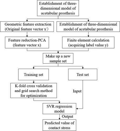
This article predicts the contact stress of the acetabular lining as shown in Figure 1:

Figure 1. Prediction process of contact stress of acetabular lining.

Finite element calculation

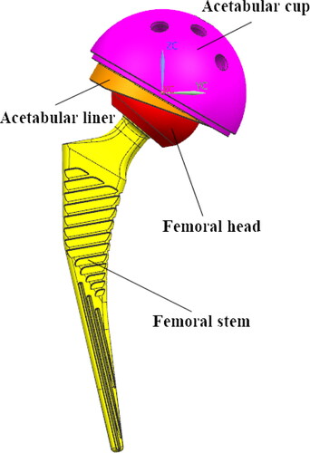
The finite element method [12] is an efficient and economical numerical simulation method, which is widely used in various industries. The finite element calculation is to prepare data for the prediction model. The acetabular stress was calculated using the method in [13], and the constraints and loads were selected for simulation according to [14]. The geometric model of the acetabular prosthesis established by unigraphics (UG) software is shown in Figure 2:

Figure 2. Geometric model.

In order to improve the calculation efficiency, the model needs to be simplified. Some insignificant details were deleted and the femoral stem neck was cut off and the part below the stem body, a small part of the neck was kept. After simplification, it is shown in Figure 3(a). A static sub-module was established using Ansys software. The material of the acetabular cup and the femoral stem was Ti6Al4V, the acetabular lining material was ultra-high molecular polyethylene, and the femoral head material was CoMoCr, respectively. The material parameters are shown in Table 1. The contact between the outer cup of the acetabulum and the lining is “bonded”. The frictional contact between the femoral head and the lining is 0.038. The constraint between the femoral stem and the femoral head is “bonded”. The mesh is hexahedral, and the mesh model is shown in Figure 3(b). Applying a fixed restraint on the neck, we allow the acetabular outer cup to move vertically and constrain other degrees of freedom, exerting a concentrated force of 1500 N on the outer surface of the acetabulum through the center of the sphere, with abduction/adduction angle −15°, flexion/extension angle −13° [14], the constrained model is shown in Figure 3(c). The lining contact stress for outputting a group of acetabular prostheses is shown in Figure 3(d).The diameters of the femoral stem, the acetabular cup and the femoral head are different for people with different physiques. To adapt to the eccentricity of different hip joints, the femoral head has "plus and minus". Although the diameter of the femoral head may be the same, the remaining dimensions are slightly different. Due to the above diversity of geometric dimensions of each group, the contact state of each group of acetabular prostheses can be different, which influences the distribution of the contact stress. Using this method, the contact stress of the other 47 groups of acetabular prostheses was calculated.

Figure 3. Finite element model.

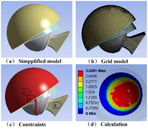
Table 1. Material properties.

Material name name	Elastic modulus	Poisson's ratio
Ti6Al4V	110Gpa	0.3
CoMoCr	925Mpa	0.45
UHMWPE	211Gpa	0.3

Support vector regression theory

Support vector regression [15] is a branch of the development of support vector machine [16], which has outstanding advantages in solving "dimensional disaster" and "over-learning". By building a training vector, a nonlinear relationship between the prediction vector and the support vector is established, and the prediction vector is forecasted. Given a training set, $T=\{(x_1,y_1),(x_2,y_2)\cdot \cdot \cdot (x_m,y_m)\},$ in which $x_i\in R^n,$ $y_i\in Y\subseteq R,$ $1\le i\le m,$ where m are the number of samples, SVR maps the input space to a high-dimensional feature space through a kernel function, and performs regression in the high-dimensional space, which is shown as follows: (1) $$f(x)=w\cdot \varphi (x)+b$$(1) where $w$ is the weight coefficient, $\varphi (x)$ is the feature space, and b is the bias term.

According to the principle of minimizing risk, the objective function can be established as follows by minimizing the weight coefficient$w$ and the bias term b [17]: (2) $$R(x)=\frac{1}{2}{\Vert w\Vert }^2+\frac{1}{m}\sum _{i=1}^m{\left|f(x_i)-y_i\right|}_{\epsilon }$$(2) where ${\left|f(x_i)-y_i\right|}_{\epsilon }$ is the loss function. In order to minimize ${\Vert w\Vert }^2$ Euler's norm and control the fitting error simultaneously, the relaxation variables ${\left\{\xi \right\}}_{i=1}^m$ and ${\left\{{\xi }^{*}\right\}}_{i=1}^m$ are introduced. The optimization problem in (2) can be transformed into a constraint minimization problem, which is: (3) $$R(x,{\xi }_i,{\xi }_i^{*})=\frac{1}{2}{\Vert w\Vert }^2+C\sum _{i=1}^m({\xi }_i+{\xi }_i^{*})$$(3) $$s.t.\{\begin{array}{c}{y}_i-w\varphi (x_i)-b\le \epsilon +{\xi }_i\\ w\varphi (x_i)+b-y_i\le \epsilon +{\xi }_i^{*},(i=1,2\cdot \cdot \cdot ,m)\\ {\xi }_i,{\xi }_i^{*}\ge 0\end{array}$$

To derive the dual problem of the original problem (Eq. (3)(3) $$R(x,{\xi }_i,{\xi }_i^{*})=\frac{1}{2}{\Vert w\Vert }^2+C\sum _{i=1}^m({\xi }_i+{\xi }_i^{*})$$(3) ), the Lagrange multipliers ${\alpha }_i,{\alpha }_i^{*},{\eta }_i,{\eta }_i^{*}$ are introduced to establish the Lagrange equation of the original problem. By partialing derivative of$w,b,{\xi }_i,{\xi }_i^{*}$ to Lagrange function, and letting the partial be 0, substituting the result into Lagrange's equation, we get the dual problem of the original problem: (4) $$\begin{array}{c}\underset{{\alpha }^{(*)}\in R^{2m}}{\min }\frac{1}{2}\sum _{i,j=1}^m({\alpha }_i^{*}-{\alpha }_i)({\alpha }_j^{*}-{\alpha }_j)[\varphi (x_i)\cdot \varphi (x_j)]\\ +\epsilon \sum _{i=1}^m({\alpha }_i^{*}-{\alpha }_i)-\sum _{i=1}^m{y}_i({\alpha }_i^{*}-{\alpha }_i)\end{array}$$(4) $$s.t.\{\begin{array}{c}\sum _{i=1}^m({\alpha }_i-{\alpha }_i^{*})=0\\ 0\le {\alpha }_i^{*}\le C,i=1,2,\cdot \cdot \cdot ,m.\end{array}$$

Therefore, the original problem is transformed into a secondary planning problem. By solving this secondary planning problem, a model of support vector regression machine can be obtained: (5) $$f(x)=w\cdot \varphi (x)+b$$(5) $$=\sum _{i=1}^m({\alpha }_i^{*}-{\alpha }_i)K(x_i,x)+b$$ where $K(x_i,x)=\varphi (x_i)\cdot \varphi (x)$ is the kernel function, $x_i$ is the training sample, $x$ is the test sample.

In theory, as long as the function meets the Mercer condition [18], it can be used as the kernel function. There are currently four kinds of kernel functions: linear kernel function, p-order polynomial kernel function, multi-layer perceptron kernel function, and Gauss radial basis kernel function (RBF). Due to the advantages of the generalization and fast calculation speed of RBF kernel functions, RBF kernel functions are more popular. The RBF kernel function can be expressed as: (6) $$K(x_i,x)=\hspace{0.17em}\text{exp}\hspace{0.17em}(-\gamma {\Vert x_i-x\Vert }^2)$$(6) where $\gamma$ is the kernel parameter.

The establishment of acetabular liner contact stress prediction model

First, feature extraction was performed on the acetabular prosthesis. For the convenience of description, the 48 groups of acetabular prostheses were numbered. The numbering rules are as follows:

1. Number according to the diameter of the outer cup of the acetabulum, from small to large;

2. There are 4 types of the size of the femoral head (S, M, L, XL). For cups with the same size, the femoral head is numbered from S-XL. Some acetabular prostheses do not have S and XL, and their numbers are numbered from small to large according to M and L.

Using this method, the 48 groups of acetabular prostheses can be numbered from 1 to 48 according to the size of the acetabular cup and the femoral head.

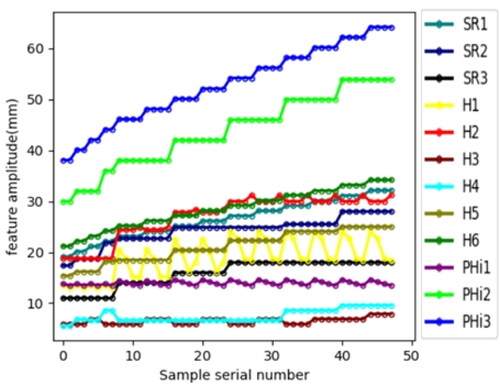
The contact stress on the acetabular liner depends on the geometrical structures of the acetabular prosthesis. Different structures and sizes cause different contact stresses of the acetabular lining. Therefore, the key dimensions of the acetabular prosthesis (e.g.：acetabular ball radius, lining ball radius, femoral head radius, acetabular thickness, etc., a total of 12 sizes) are used as the feature data $x^{\prime }$ of the sample data. The schematic diagram of its characteristics is shown in Figure 4. The sample features are shown in Figure 5.

Figure 4. Sample features.

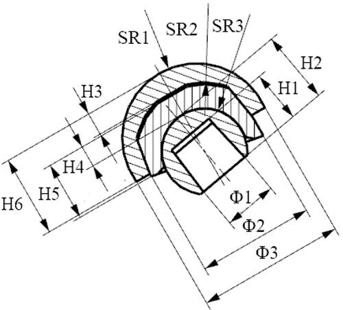
Figure 5. Sample features.

Feature dimensionality reduction

Due to the large number of features (12 features) and the small number of samples (48 samples), in order to fully learn the hyperparameters, the feature vector needs to be reduced in dimension. Principal Component Analysis (PCA) is a commonly used linear dimensionality reduction method. Its basic idea is to map high-dimensional data to low-dimensional data space through linear projection; it is not data for high-dimensional data. For the reduction, the low-dimensional integration and reconstruction is carried out. After the low-dimensional features are obtained, the feature vectors that have the most influence are retained, so that the amount of data information lost is very small.

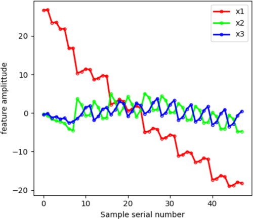
The reconstructed feature is recorded as x. According to the experiment, when the feature dimension is 3, the prediction effect is the best, the feature contribution rate is [0.9375, 0.03646, 0.01680], and the total contribution rate has reached 99.07%, and the amount of information reduction on the original feature is very small. The feature after dimensionality reduction has lost its original physical meaning, and the three feature components are$x_1,x_2,x_3,$ respectively; the feature after dimensionality reduction is shown in Figure 6.

Figure 6. Features after dimensionality reduction.

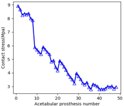
The calculation result of the finite element as the label value of the sample data is counted as y, as shown in Figure 7.

Figure 7. Contact stress of acetabular prosthesis.

Then we trained the support vector regression machine, randomly abstracted 80% of the data from 48 samples for training. The remaining 20% are used as test samples. During the training process, C and $\gamma$ in the support vector regression machine need to be optimized to obtain a high-precision prediction model. In this paper, K-fold cross validation [19] was used combined with the grid search method [20] to obtain the optimal C and$\gamma$ values.

Results

Acetabular contact stress prediction

Through parameter optimization, the optimal values of C and$\gamma$ are finally obtained, which are C = 23.3 and $\gamma$ = 0.01, respectively. We input the test data to the prediction model, then the prediction results are obtained, as shown in Figure 8.

Figure 8. Prediction results.

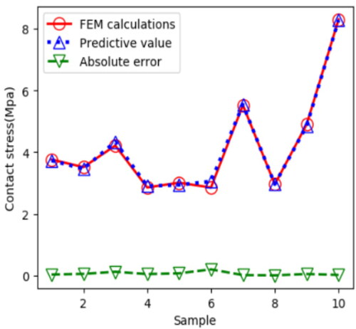
Note: The red line represents the calculated value of the finite element, the blue line represents the predicted value, the green line represents the absolute error between the calculated value and the prediction, respectively.

It can be seen from Figure 8 that the prediction effect of the model is very good, and the maximum absolute error is only 0.1986.

Model performance evaluation

In order to evaluate the prediction model, we use the two factors of determination coefficient (R²) and root mean square error (RMSE) [21]. The root mean square error and the coefficient of determination are established by the following formula: (7) $$R^2=1-\frac{\mathit{RSS}}{\mathit{TSS}}$$(7)

Where: $\mathit{TSS}=\sqrt{{\sum }_{i=1}^n{(y_i-\overline{y})}^2},$ $\mathit{RSS}=\sqrt{{\sum }_{i=1}^n{({\widehat{y}}_i-y_i)}^2}$ (8) $$\mathit{RMSE}=\sqrt{\sum _{i=1}^n{({\widehat{y}}_i-y_i)}^2/n}$$(8) where $y_i$ is the calculated value of finite element,${\widehat{y}}_i$ is the sample predicted value, $\overline{y}$ is the sample mean, n is the number of samples, respectively.

The smaller the RMSE and the larger R², the better the prediction effect (1 is the best). According to the formulas (7) and (8), the RMSE of the prediction model is 0.09309, and the R² is 0.9426.

In order to verify the superiority of the model, the prediction results of this model are compared with Ridge regression and Lasso models. The comparison of prediction results is shown in Figure 9, and the evaluation index pair is shown in Table 2.

Figure 9. Comparison of prediction results.

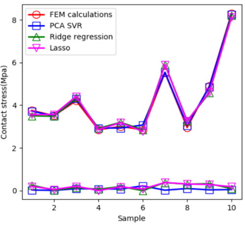
Table 2. Model performance comparison standard table.

Project	RMSE	R²
PCA-SVR	0.09309	0.9426
Lasso	0.2634	0.8647
Ridge regression	0.2635	0.8647

It can be seen from Figure 9 that the method proposed in this paper can more accurately predict the contact stress of the acetabular lining with the smallest absolute error. From Table 2 it can be seen that the prediction capabilities of Lasso and Ridge regression are equivalent, while the RMSE value of the method proposed in this paper is the smallest, R² Obviously larger than the other two models, which shows that the proposed method has higher prediction accuracy.

Discussion

Using support vector regression to make predictions has been widely used in various industries. Many scholars have made contributions; to name a few, Karmy and Maldonado [22] applied the SVR method to sales forecasting projects in the tourism retail industry, and pointed out that the SVR method is superior to the ARIMA and Holt-Winters methods in forecasting performance. Lu et al. [23] uses SVR to establish a CFRP structure. The damage degree prediction method provides a feasible method for the prediction of the damage degree of CFRP structure. Xue et al. [24] proposed an AUKF-GA-SVR method, which effectively solved the inaccuracy issue in the prediction of the remaining useful life (RUL) of the lithium ion battery. The studies of the above scholars have proved the superiority of the SVR method in predicting performance. From the perspective of the prediction effect in this study, the accuracy of the PCA-SVR method for acetabular prosthesis contact stress prediction model established in this paper is the best. It illustrates that the use of the feasibility of predicting the contact stress of the external structural characteristics of the acetabular prosthesis will also reduce the workload of the R&D personnel and greatly advance the development progress.

However, the method in this paper also has a shortcoming: the training set and test set data are derived from finite element calculations, and the actual experimental data cannot be obtained. Therefore, the model established can only be used for screening of "worst-case" acetabular prosthesis models, and it cannot be used to evaluate whether our products are qualified. The actual experimental data will be included in the next research plan; with the measured data, subsequent research and development of related products will greatly reduce costs.

Conclusions

This paper presents a method for predicting the contact stress of the acetabular lining based on support vector regression machine learning. The prediction results of the test data show the effectiveness of the prediction model. From the calculation results of the finite element method, it can be known that the contact stress of the acetabular lining decreases with the increase of the external dimension of the acetabular outer cup. This will give us a general direction for the selection of the "worst case" of wear. The RMSE value of the prediction model is 0.09309 and the R² value is 0.9426. The prediction performance of the proposed method is compared. The results show that the prediction performance of the proposed method is significantly better than Lasso and Ridge regression. At the same time, it is used for product improvement and design of the same series of products. Provides guidance on the "worst case" selection of wear.

Disclosure statement

No potential conflict of interest was reported by the authors.

Data availability

The data that support the findings reported in this study are available from the corresponding author upon reasonable request.

Additional information

Funding

This study was supported by the National Natural Science Foundation of China (NSFC, grant number 11362020).

References

- Maxian TA, Brown TD, Pedersen DR, et al. A sliding-distance-coupled finite element formulation for polyethylene wear in total hip arthroplasty. Techn Note. 1996;29(5):687–692.
- Wang L, Liu XH, Li DC, et al. Contact mechanics studies of an ellipsoidal contact bearing surface of metal-on-metal hip prostheses under micro-lateralization . Med Eng Phys. 2014;36(4):419–424.
- Hua X, Li JJ, Jin ZM, et al. The contact mechanics and occurrence of edge loading in modular metal-on-polyethylene total hip replacement during daily activities. Med Eng Phys. 2016;38(6):518–525.
- Cilingir AC. Finite element analysis of the contact mechanics of ceramic-on-ceramic hip resurfacing prostheses. J Bionic Eng. 2010;7(3):244–253.
- KošakKralj-Iglič RV, Iglič A, et al. Polyethylene Wear is Related to Patient-specific Contact Stress in THA. Clin Orthop Relat Res. 2011; 469(12):3415–3422.
- Lizhang J, Fisher J, Jin Z, et al. The effect of contact stress on cartilage friction, deformation and wear. Proc Inst Mech Eng H. 2011; 225(5):461–475.
- Jangid V, Singh A, Mishra KA. Wear Simulation of artificial hip joints: effect of materials. Mater Today Proc. 2019; 18:3867–3875.
- Balabin RM, Lomakina EI. Support vector machine regression (SVR/LS-SVM)-an alternative to neural networks (ANN) for analytical chemistry? Comparison of nonlinear methods on near infrared (NIR) spectroscopy data . Analyst. 2011; 136(8):1703–1712.
- Guo F, Ren LH, Jin YC, et al. A dynamic SVR–ARMA model with improved fruit fly algorithm for the nonlinear fiber stretching process. Nat Comput. 2019;18(4):747–756.
- García-Nieto PJ, García-Gonzalo E, Sánchez Lasheras F, et al. A hybrid DE optimized wavelet kernel SVR-based technique for algal atypical proliferation forecast in La Barca reservoir: a case study. J Comput Appl Math. 2020;366:112417.
- Li Y, Sun MH, Yan WZ, et al. Multi-output parameter-insensitive kernel twin SVR model. Neural Netw. 2020;121:276–293.
- DundarTopkaya ST, Solmaz MY, et al. Finite element analysis of the stress distributions in peri-implant bone in modified and standard-threaded dental implants. Biotechnol Biotechnolog Equip. 2016;30(1):127–133.
- Hua X, Wroblewski BM, Jin ZM, et al. The effect of cup inclination and wear on the contact mechanics and cement fixation for ultra high molecular weight polyethylene total hip replacements. Med Eng Phys. 2012;34(3):318–325.
- ISO 14242-3. 2009. Implants for surgery — Wear of total hip-joint prostheses — Part 3: loading and displacement parameters for orbital bearing type wear testing machines and corresponding environmental conditions for test.Avilable from https://www.iso.org/standard/44997.html.
- Chang CC, Lin CJ. LIBSVM: a library for support vector machines. ACM Trans Intell Syst Technol. ). 2011; 2(3):1–65.
- Wu CH, Tzeng GH, Lin RH. A novel hybrid genetic algorithm for kernel function and parameter optimization in support vector regression. Expert Syst Appl. 2009;36(3):4725–4735.
- Smola AJ, Schölkopf B. A tutorial on support vector regression. Statist Comput. 2004;14(3):199–222.
- Kavousi-Fard A, Samet H, Marzbani F. A new hybrid modified firefly algorithm and support vector regression model for accurate short term load forecasting. Expert Syst Appl. 2014;41(13):6047–6056.
- Ling H, Qian CX, Kang W, et al. Combination of support vector machine and K-Fold cross validation to predict compressive strength of concrete in marine environment. Constr Build Mater. 2019;206:355–363.
- Chen HZ, Liu ZY, Cai K, et al. Grid search parametric optimization for FT-NIR quantitative analysis of solid soluble content in strawberry samples. Vib Spectrosc. 2018;94:7–15.
- Tutun S, Chou CA, Canıyılmaz E. A new forecasting framework for volatile behavior in net electricity consumption: a case study in Turkey. Energy. 2015;93:2406–2422.
- Karmy JP, Maldonado S. Hierarchical time series forecasting via support vector regression in the European Travel Retail Industry. Expert Syst Appl. 2019;137:59–73.
- Lu SZ, Jiang MS, Wang XH, et al. Damage degree prediction method of CFRP structure based on fiber. Optik. 2019;180:244–253.
- Xue Z, Zhang W, Cheng YC, et al. Remaining useful life prediction of lithium-ion batteries with adaptive unscented kalman filter and optimized support vector regression. Neurocomputing. 2020;376:95–102.