Distinguishing areas of organic, biodynamic and conventional farming by means of multispectral images. A pilot study

Abstract

The aim of the present investigation was to develop a basic methodological scheme for distinguishing organic, biodynamic and conventional areas of winter wheat cultivation, based on the satellite images from Sentinel-2. The target areas are located in the experimental field of the Institute of Agriculture in Karnobat, Bulgaria. The plant condition was determined on a three-point rating scale according to the average plant height, percentage of projective cover of the aboveground plant parts and intensity of the green color of leaves during the end of tillering to complete ripeness. To determine the homogeneity of the target polygons, we used a small drone DJI Phantom 4, with 1/2.3 CMOS camera and Dronedeploy to compile flight plans for shooting and photogrammetric processing of the images. ArcGIS was used in GIS procedures and analyses. Microsoft Excel, with Solver ADD-IN was used to clusterize the target polygons in order to distinguish the polygons of organic, biodynamic and conventional farming by the multispectral indices (CRI 1, MSAVI, NDVI, NDWI, PSSRa, PSSRc, WDRVI). All selected indices were calculated in GIS environment. Ground observations showed that there were differences in the condition of plants in different cultivation systems during the selected observation phases. The obtained results reveal that the differences in dynamics and development during the growth and development stages of the wheat in the organic, biodynamic and conventional fields can be traced by spectral characteristics from satellite images and they can be used to distinguish them.

Keywords:

• Multispectral satellite images
• spectral indices
• distinguishing areas
• organic
• biodynamic
• conventional farming
• wheat

Introduction

Remote sensing methods which use multispectral satellite images and suitable spectral indices are part of the modern tools for solving various problems related to land cover and agrocenoses in particular. They can help distinguish areas of different crops [1–5], determine the propagation of economically significant weeds [6], pests [7] and diseases such as wheat yellow rust in wheat [8]. Babar et al. [9] found that the spectral reflectance index has the potential to differentiate spring wheat breeding lines under irrigated conditions and in this case the most suitable for distinction were the heading stage and the grain-filling stage.

Based on the data from 12 channels of multispectral satellite cameras, a large number of indices have been developed. Over two hundred of these indices were summarized by Henrich et al. [10]. Some of them reflect the dynamics of plant pigments or soil characteristics. Along with widely used indices such as Normalized difference vegetation index (NDVI), Carotenoid reflectance index (CRI1), Normalized Difference Water Index (NDWI), Pigment specific simple ratio-Chla (PSSRa), Pigment-specific simple ratio (PSSRc) [4, 11,12], particular interest is also paid to Modified Soil Adjusted Vegetation Index (MSAVI) and Wide Dynamic Range Vegetation Index (WDRVI). For a better physiological and phenological characterization of the crops in conditions of moderate to high density, Gitelson [13] proposes WDRVI, as a modification of NDVI. In WDRVI the same spectral lines as in NDVI are used, adding a coefficient which takes values from 0.1 to 0.2 depending on the vegetation density. Leaf area index (LAI) is a key biophysical variable, which is used to obtain agronomic information on field management and yield predictions. Wu et al. [14] in their LAI studies established that MSAVI give the best results. It manifests the largest dynamic range and the highest sensitivity and overall efficiency when tested on maize and potatoes. In their investigation on four mixed grassland communities, He et al. [15] found that Adjusted transformed soil–adjusted vegetation index (ATSAVI) was the most suitable among the indices they approbated.

In recent years in Europe there has been a growing demand for stable crop production and striving for reduction of the inputs of pesticides and synthetic fertilizers and for biodiversity increasing. This demand is reflected in the efforts to integrate environmental aspects into the Common Agricultural Policy (CAP). Organic farming is the strictest production system with low-input defined by Council Regulation (EEC) No 2092/91 (http://www.fao.org/faolex/results/details/en/c/LEX-FAOC002355/). The production of organic food in European Union (EU) countries is expected to grow steadily in the next years due to the new more ambitious goals of the EC for healthier and more sustainable EU food system set out in the European Green Deal. To achieve these goals in the Farm to Fork Strategy it is envisaged at least 25% of the EU’s agricultural land to be under organic farming by 2030.

In order to ensure greater reliability and security for the consumers of organic products, a system of control and certification has been introduced, including traceability of the technological processes to the final agricultural products in the organic farms. On the other hand, certification control is one of the conditions that organic farmers must meet in order to benefit from financial support through subsidies. The certification process is difficult, time- and labor-consuming including field inspections. Therefore, the control is based mainly on documentary and accounting inspections and very few parcels are subject to field observations. The development of the regulatory framework and the requirements to organic agriculture, together with the possibilities for effective and precise control by certifying institutions, ensure improvement of the quality of agricultural produce. The development of remote sensing methods for distinguishing of organic areas can facilitate and complement the control in the certification and subsidies receiving and help certification bodies to cope with the growing number of organic crop areas to certify.

The prerequisites for creating a methodology for remote recognition of organic fields distinguished from conventional ones are:

• organic fields differ from conventional ones due to different management practices by various characteristics, the main ones being lower crop biomass and the rates of plant development, lower plant nitrogen and chlorophyll concentration, higher intrafield heterogeneity of the canopy and a higher soil organic matter content [16,17];

• free access to weekly high-resolution satellite multispectral data from Sentinel-2;

• a number of developed spectral indices, which combine data from satellite camera channels and are widely used in precision agriculture;

• accessible software and hardware tools for working with multispectral raster images in GIS environment;

• accessible possibilities to receive orthophotographic images taken with small drones, which are necessary for additional refinement of the target polygons.

The implementation of such a methodology will facilitate the certification process, improve public confidence in organic foods and will eventually further boost the production of more healthy foods.

The working hypothesis was that crops grown in conventional, organic and biodynamic¹ farming can be reliably distinguished by means of data from multispectral satellite images and using precise target polygons and suitable analytical apparatus.

The aim of this paper was to develop a basic methodological scheme, based on the images from Sentinel-2, to distinguish organic, biodynamic and conventional areas of winter wheat.

Materials and methods

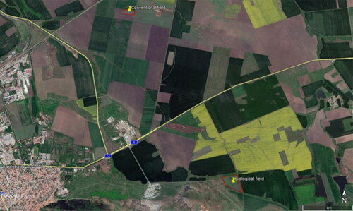
The target areas are located in the experimental field of the Institute of Agriculture (Agricultural Academy) in Karnobat, Bulgaria (Figure 1). They satisfy the requirements to have very close agroclimatic conditions and soil type.

Figure 1. Target areas in the experimental field of the Institute of Agriculture, Agriculture Academy, Karnobat, Bulgaria.

Brief description of the organic and conventional experimental areas

In the experimental field in the region of Karnobat, organic farming has been applied for 12 years and biodynamic, for 6 years. Experiments have been conducted in the conventional experimental field since 1925, when the Institute of Agriculture was founded.

Brief description of the region

The experimental field for the organic and biodynamic fields is located on a land plot with cadaster No 146001, with an area of 7.14 ha (Figure 1). The field borders on four sides are a field-protective forest belt. It does not border farming lands where farming crops are grown by means of conventional methods. The conventional field is located in the Glumche locality, some 4 km from the experimental organic and biodynamic fields.

The soils of the experimental fields are Eutric Vertisols [20]. They are characterized as:

• well-supplied with mobile potassium (24–28 mg/100 g),

• medium supplied with mobile phosphorus (3.3–4.7 mg/100 g), and

• poorly supplied with mineralizable nitrogen (30–40 mg/1000 g) [21].

The altitude of the organic field is 251–276 m, and of the conventional one, 160–170 m.

The climate in the region of Karnobat is transitional-continental. North and southwest winds are prevalent in the region. During the summer months in the afternoon hours, the sea breeze also reaches the region and has a beneficial impact on the growth and development of the agricultural crops.

The average annual air temperature is 11.5°С. The coldest months are January, February and December, and the hottest ones are July and August. The absolute minimum air temperature measured in Karnobat is −26°С, and the absolute maximum is +42.0°С. The precipitation in the region of Karnobat ranges from 302 mm in 1945 to 880 mm in 2014 and 990 mm in 2018. The average annual precipitation is 551 mm. The wettest months are May and June, and the driest periods are August-September and February-March. The average duration of snow cover is 23 days. The average long-term relative air humidity ranges from 63% in August to 85% in December [22,23].

The experimental fields were sown with Miryana, a common winter wheat variety created at the Institute of Agriculture in Karnobat. It is intended for use in conditions typical of the Balkan Peninsula in fields with elevation of up to 700 m.

The agricultural practices performed in the conventional, organic and biodynamic fields are presented in Table 1. In the organic and biodynamic field, the pest control was conducted with preventive measures (crop rotation, optimal sowing, early harvest, good quality seed, etc.). Manure was applied to the biodynamic field in September. In the spring of vegetation year 2019, phytosanitary monitoring was also conducted on the fields (Table 2).

Table 1. Agricultural practices in the experimental fields.

Type of procedure		Type of farming
		Conventional	Organic	Biodynamic
Fertilization	Type of fertilization	Ammonium nitrate (NH4NO3), Active substance content – total nitrogen (N) – 34.4%	None	Manure
	Rate	30 kg/da		5 t/da
	Date	9th February 2019		September 2018
Chemical protection	Type of preparation	Herbicides Granstar Super (250 g/kg Tribenuron-methyl + 250 g/kg Thifensulfuron methyl) + Scorpio Super 7.5 EW (69 g/L Fenoxaprop-P-ethyl + Antidote)	None	None
	Doses	4 g/da; 100 g/da
	Date	17th Apr 2019
	Type of preparation	Fungicide + insecticide Falcon (167 g/L tebuconazole + 250 g/L spiroxamine + 43 g/L triadimenol) + Sherpa 100 EW (100 g/L cypermethrin)	None	None
	Doses	60 mL/da + 25 mL/da
	Date	9th May 2019

Table 2. Biotic characteristics of the experimental fields.

Biotic characteristics		Type of farming
		Conventional	Organic	Biodynamic
Diseases	Nematodes	0	0	0
	Powdery mildew	1	1	1
	Septoria, rust	2	1	1
Pests	Insects	2	1	1
	Rodents (calamities)	1	0	0
Weeds *	Polygonum convolvulus L.	0	2	1
	Caucalis daucoides L.	0	2	0
	Veronica hederifolia L.	1	2	1

Note: The rating is on a four-point scale: 0 none; 1 weak; 2 medium; 3 strong.

* The top three most significant weeds are presented, according to expert assessment.

Field data for control sites

1. The plant condition was determined on a three-point rating scale: very good (3) good (2) poor (1) . For this purpose we reported the average plant height, percentage of projective cover of the aboveground plant parts and intensity of the green color of leaves on a four-point scale: saturated (4), normal (3) pale (2), yellowing (1). The plant condition was monitored from the end of tillering (3rd Apr 2019) to complete ripeness (4th Jul 2019).

2. The area occupied with plants damaged by pests and diseases is presented in %.

Software used

ArcGIS desktop 10.6

ArcGIS was used in GIS procedures and analyses.

Dronedeploy

Dronedeploy was used to compile flight plans for the drone autopilot for shooting and photogrammetric processing of the images obtained by the drone resulting in images for RGB, Plant Health and Elevation.

Microsoft Excel, with Solver ADD-IN -Microsoft Excel was used to clusterize the target polygons in order to distinguish the polygons of biological and conventional agriculture by the multispectral indices based on satellite images.

Aerial images

To determine and precise relatively homogenous target polygons, images were taken immediately before the end of tillering (25–27th March) and the beginning of earing (15–16th April) with a small DJI Phantom 4 drone, with camera with 1/2.3″ CMOS, effective pixels: 12.4 M, from a height of 50 m.

Selection of satellite images

Four multispectral satellite images were used from the pair of European satellites Sentinel-2, with atmospheric correction and without clouds above the target area on:

• 3rd April 2019 L2A_T35TNH_A019738_2019 04 03 T090019

• 26th May 2019 L2A_T35TMH_A020496_2019 05 26 T090557

• 17th June 2019 L2A_T35TMH_A011902_2019 06 17 T090059

• 25th June 2019 L2A_T35TMH_A020925_2019 06 25 T091818

In the selection of dates we used all available cloudless images in spring and summer. During this period, the conditions for distinguishing the conventional from the organic and biodynamic areas were most suitable, because at that time the type of agriculture had the greatest impact on the projectile cover of young plants, on the one hand, and on the differences in plant pigment composition, on the other.

Multispectral indices used

Having considered the characteristics of the used variety of winter wheat (biological and physiological characteristics, climatic and soil conditions in the region) and the need of greatest detail in the images for the channels used, the number of suitable indices was limited to seven: Carotenoid reflectance index (CRI1); Modified soil adjusted vegetation index (MSAVI), Normalized difference vegetation index (NDVI), Normalized difference water index (NDWI), Pigment specific simple ratio Chla (PSSRa), Pigment-specific simple ratio (PSSRc) and Wide dynamic range vegetation index (WDRVI). The formulas for the selected indices are presented in Table 3. For each of these indices 10-meter resolution channels from Sentinel-2 were used.

Table 3. Used spectral indices.

Index	Name of index	Formula	References
CRI 1	Carotenoid reflectance index	1/B02 − 1/B03	Gitelson et al. [13]
MSAVI	Modified Soil Adjusted Vegetation Index		Qi et al. [4]
NDVI	Normalized difference vegetation index [800,680]	(B08–B04)/(B08 + B04)	Rouse et al. [5]
NDWI	Normalized Difference Water Index	(B03–B08)/(B03 + B08)	McFeeters [12]
PSSRa	Pigment specific simple ratio Chl a	B8/B4	Blackburn [11]
PSSRc	Pigment-specific simple ratio	B8/B2	Blackburn [11]
WDRVI	Wide Dynamic Range Vegetation Index	(a*B08–B04)/(a* B08 + B04); a from 0.1 to 0.2	Gitelson et al. [13]

Procedure to determine target areas and target polygons in GIS

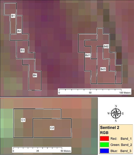
The photogrammetric image taken by a drone initially outlined the target areas in a shapefile, Figure 2. The area borders were attached to the borders of the satellite pixels, Figure 3.

Figure 2. Target polygons with drone images: organic (B1, B2, B3, B4); biodynamic (Bd1, Bd2, Bd3); conventional (C1 and C2).

Note: A – True colors (RGB) organic and biodynamic polygons; B – Elevation (RGB) organic and biodynamic polygons; C – Plant Health (RGB) organic and biodynamic polygons; D – True colors (RGB) conventional polygons; E – Elevation (RGB) conventional polygons; F – Plant Health (RGB) conventional polygons

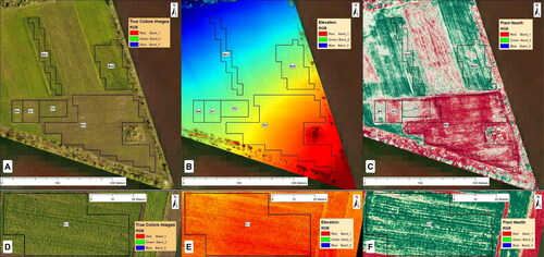
Figure 3. Connecting the boundaries of target polygons with the boundaries of satellite pixels.

The ten-meter resolution of the satellite images also implied the presence of heterogeneous pixels in terms of visible roads, bushes, field boundaries, grass areas around single trees or utility poles, shafts and other objects. In addition, heterogeneity could be related to microrelief, erosion spots and stonier spots, terrain slope and exposure, situation in relation to the catchment slope, and crop density. Heterogeneity above a certain level can lead to distortion of the spectral characteristics of the satellite images and consequently to the reliability in distinguishing the different types of fields. Therefore, such heterogeneous pixels were removed from the analysis. In order to identify the heterogeneous pixels, the detailed photogrammetric image captured by the drone and the products obtained from it (TCI, Elevation and Plant health) were used. We consider as heterogeneous pixels the ones where, according to expert estimates, heterogeneity affects more than 10% of its total area.

Calculation of indices in GIS environment

The following methodology was used to calculate the indices in the GIS environment:

1. Cropping the raster images from satellite pictures by means of the Extract by Mask tool, and using the shapefile with the target polygons obtained by the above procedure as a template. Thus, the size of the rasters to be used is reduced from 10,000 km² to under 0.000000 1 km², which speeds up the calculations manyfold.

2. Calculation of the indices for the received rasters with the respective target polygons. The calculation can be done manually separately for each index with the Raster calculator tool in ArcGIS, but the values for each index were obtained by means of a Python script and raster algebra (the script equivalent of the raster calculator) which is both faster and less error-prone.

3. Calculation of the mean values for each polygon by indices. For each index and each date Zonal statistics as table was used. The table obtained in this way was then connected with the attribute table of the polygon layer. The values in column Mean were transferred to column {index}_{date} of the attribute table and finally the connection was removed.

4. Standardizing the index data.

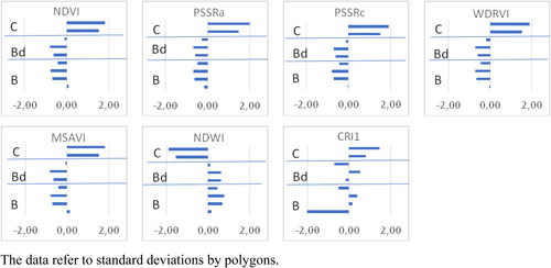
Diagrams for the standard deviation were made by dates after standardizing each index and are illustrated in Figure 4 for 26th May.

Figure 4. Diagrams for the 7 indices after standardization, 26th May.

Clusterization of target polygons

Clusterization procedure

Microsoft Excel with Solver add-in was used to determine the polygons which would be cluster centers. The program first postulated the number of clusters according to the nature of the source data. The number of clusters was determined by the types of polygons in the field experiment. The program ran different variants in order to select polygons for cluster centers which minimized the sum of squared errors (SSE). In the four periods of the study each index was standardized with regards to its Mean and Standard Deviation values so that the indices would be comparable as axes in multidimensional space.

The distance between each pair of polygons in 7-dimensional space was computed by taking the square root of the sum of squares of differences. The formula = SQRT(SUMXMY2(A2:G2;A4:G4)) computes the distance between polygons standardized index values arranged horizontally in rows 2 and 4. The polygons were clustered based on their spectral characteristics presented by the used spectral indices. When a polygon was selected as a cluster center, it kept its type in the cluster created around it, and the type of the central polygon was assigned to the rest of the cluster polygons.

In this regard, the following consecutive actions were performed:

• Specifying the number of clusters. It equals the number of polygon types according to the set field experiment. In our case, the clusters are three, corresponding to three different managed fields: conventional, biodynamic and organic.

• Entering the index values by dates for each polygon.

• Indication of the polygon type according to the type of farming applied to them.

When a polygon is selected as a cluster center, it keeps its type in the cluster created around it and the type of the central polygon is assigned to the rest of the cluster polygons. After setting the number of groups, respectively the number of central polygons in multidimensional space, the algorithm determines the central polygon in each of them. If among the central polygons there are two of the same type (regardless whether it is organic, biodynamic or conventional), this automatically leads to separation of the polygons of this type into different clusters and objectively then no complete separation can be achieved.

Results

In situ observations of experimental fields

The period of the experiment was droughty, especially during the autumn-winter season. In October, December, February and March, the precipitation was far below the norm (Table 4). This created difficulties for the normal development of the wheat plants. At the time of first observation (April 3rd, 2019) the wheat plants in the conventional field were better developed, with larger biomass compared to those in the organic field; therefore the former began to suffer more from the deficiency of air and soil moisture. The crops in the organic and biodynamic fields were less developed, with lower biomass, but had better turgor and tolerated drought better. The precipitation in April, May and June managed to compensate to a large extent the delay in the development of wheat in the conventional field. Thus the observation on 17th June can be considered as conducted under favorable conditions for the three types of polygons.

Table 4. Average monthly precipitation, mm, of 2018/2019 years and long-term average (1901-2020) in Karnobat.

Vegetation period	X	XI	XII	I	II	III	IV	V	VI	VII	VIII	IX	⅀
Long-term average (1901–2010), [mm]	45.2	53.4	52.1	36.1	36.7	33.4	46.2	59.7	63.2	47.9	34.3	42.7	551
2018/2019, [mm]	15.4	68.3	27.3	38.9	15.6	8.9	52.9	44.9	95.6	33.7	13.8	19.3	435

The plant condition rated based on average plant height, percentage of projective cover of the aboveground plant parts and intensity of the green color of leaves, was identified as very good (3) [11] in the conventional and biodynamic field and as good (2), in the organic field. Тhe organically grown plants were shorter (81.0 cm average plant height) than the conventionally (91.5 cm) and the biodynamically (93.1 cm) grown ones. The percentage of projective coverage of the aboveground plant parts in the conventional field was the highest (90%), in the biodynamic field, slightly lower than 85% and in the organic one, the lowest (75%). In the conventional and the biodynamic fields the intensity of green color of the leaves was similar, and was determined as normal green color based on the visual scale [11]. In the organic field the plants were with pale green color of the leaves [9], which is indicative of insufficient nutrients and nitrogen in particular.

According to field data, in the control sites, there were no expressed negative effects from diseases, pests or weeds in the crops of the three types of cultivation that vegetation year (Table 2). The period from 14th Apr 2019 (the date of the first treatment with plant protection products in the conventional field) to 17th Jun 2019 (the date with the best separation of the polygon types) was sufficient to register diseases, pests and weeds in the three types of farming. Although no fungicides or insecticides had been applied in the organic and biodynamic fields, the observed rate of attack by major diseases and pests was at the same level or even lower than in the conventional field.

Determination of target areas and target polygons in GIS

The borders of the target areas grown in different ways and the target polygons within them were determined in GIS according to the above described procedures and criteria (Figure 2). The selection was made based on the presence of relatively homogenous pixels from each target area. In the organic field the target polygons were from B1 to B4, in the biodynamic field the target polygons were from Bd1 to Bd3, in the conventional field they were C1 and C2. The areas of the target polygons and the predecessors before growing wheat are presented in Table 5.

Table 5. Areas of target polygons.

Polygon	Type	Code	Predecessor	Area [m^2]
1	Conventional	C1	Pea	900
2	Conventional	C2	Pea	800
3	Biodynamical	Bd1	Pea	1 300
4	Biodynamical	Bd2	Pea	1 700
5	Biodynamical	Bd3	Pea	1 200
6	Organic	B1	Pea-sunflower mix	700
7	Organic	B2	Pea-sunflower mix	600
8	Organic	B3	Pea-sunflower mix	700
9	Organic	B4	Pea-sunflower mix	1 100

Calculation of indices in GIS environment

The mean values of all spectral indices used were calculated for all polygons and for each of the 4 survey dates. The original values of the 7 spectral indices used by target polygons are illustrated with the data for 26th May and 17th June (Table 6). The ATSAVI index, which showed good results for solving the problem under consideration, was excluded from further research as high correlation with the NDVI index was established after the standardization procedure. All indices had lower values at a later study observation date (17th June) in all target areas except for the indices NDWI (Normalized Difference Water Index) and CRI1 (Carotenoid reflectance index). The variation in the values was larger in the organic polygons than in the conventional and the biodynamic polygons and is due to the greater intrafield heterogeneity of the canopy under organic conditions. The NDVI index values for all target polygons during the observation on 17th June are also presented as raster graphic in Figure 5. The raster images illustrate visually the differences in the physiological and phenological development of wheat plants from the same variety in the differently managed fields, on the one hand, and on the other, the variation of studied indices among the different polygons in one field.

Figure 5. Rasters with NDVI values by pixels.

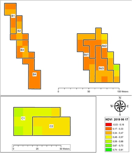
Table 6. Original index values by target polygons.

Date	N	NDVI	WDRVI	NDWI	PSSRa	PSSRc	CRI1	MSAVI
26th May	1	0.70	−0.28	−0.61	5.68	6.88	−0.11	0.82
	2	0.65	−0.36	−0.57	4.69	5.82	−0.05	0.79
	3	0.64	−0.37	−0.57	4.58	5.68	−0.04	0.78
	4	0.66	−0.33	−0.59	5.00	6.22	−0.07	0.80
	5	0.65	−0.35	−0.58	4.79	5.95	−0.06	0.79
	6	0.64	−0.37	−0.58	4.58	5.84	−0.04	0.78
	7	0.69	−0.30	−0.61	5.45	6.71	−0.07	0.81
	8	0.80	−0.05	−0.71	9.12	9.22	−0.03	0.89
	9	0.82	0.01	−0.73	10.21	9.87	−0.02	0.90
17 th June	1	0.25	−0.71	−0.41	1.68	3.64	0.17	0.40
	2	0.24	−0.72	−0.41	1.64	3.44	0.21	0.39
	3	0.25	−0.72	−0.41	1.65	3.35	0.24	0.39
	4	0.23	−0.73	−0.41	1.59	3.41	0.22	0.37
	5	0.25	−0.71	−0.43	1.69	3.74	0.20	0.41
	6	0.31	−0.67	−0.47	1.97	4.26	0.18	0.47
	7	0.26	−0.71	−0.45	1.69	3.80	0.22	0.41
	8	0.49	−0.55	−0.56	2.93	6.49	0.02	0.65
	9	0.43	−0.60	−0.53	2.49	5.92	0.04	0.60

Clustering procedures

Initially, in the clustering procedure, three clusters were postulated, corresponding to three observed fields: conventional, organic and biodynamic.

For two of the four observation dates (April 3rd, May 26th) different polygons were identified for cluster centers (Table 7). For 3rd April the central polygons were one biodynamic (Bd1) and two conventional ones (C1 and C2); for 26th May, one organic (B2), one biodynamic (Bd3) and one conventional (C1). For 17th June and for 25th June the identified central polygons were the same: one biodynamic (Bd1) and two conventional (C1 and C2). For three of the dates (April 3rd, June 17th and June 25th) the algorithm specified both conventional polygons (C1 and C2) as cluster centers. For all dates all conventional polygons were recognized by analyses such as they really are. All biodynamic polygons were also correctly determined on three of the observation dates, but on 26th May two of them were recognized as organic. The organic polygons were not correctly determined by analyses for all dates, except for two polygons on May 26th. On the two last days of observation (June 17th and 25th) they were recognized as biodynamic, whereas on April 3rd two of them, as conventional ones, and two as biodynamic.

Table 7. Distances from polygons to the centers of the three clusters.

N	Code	Original type	3rd April					26th May
			Cluster centers			Min	Recognized type	Cluster centers			Min	Recognized type
			Bd1	C1	C2			B2	Bd3	C1
1	B1	B	0.06	47.51	14.69	0.06	Bd1	7.32	1.82	22.18	1.82	Bd3
2	B2	B	14.19	9.46	0.06	0.06	C2	0.00	2.46	29.07	0.00	B2
3	B3	B	17.10	7.85	0.28	0.28	C2	0.09	3.45	31.08	0.09	B2
4	B4	B	2.68	27.16	4.50	2.68	Bd1	0.77	0.59	24.77	0.59	Bd3
5	Bd1	Bd	0.00	46.47	14.00	0.00	Bd1	0.13	1.63	28.00	0.13	B2
6	Bd2	Bd	3.04	26.13	4.21	3.04	Bd1	0.18	3.60	30.12	0.18	B2
7	Bd3	Bd	2.95	72.10	29.54	2.95	Bd1	2.46	0.00	18.85	0.00	Bd3
8	C1	C	46.47	0.00	9.70	0.00	C1	29.07	18.85	0.00	0.00	C1
9	C2	C	14.00	9.70	0.00	0.00	C2	40.78	29.46	1.28	1.28	C1
	SSE					9.07		SSE			4.08
N	Code	Original type	17th June					25th June
			Cluster centers			Min	Recognized type	Cluster centers			Min	Recognized type
			Bd1	C1	C2			Bd1	C1	C2
1	B1	B	0.33	42.41	24.26	0.33	Bd1	0.13	47.22	18.15	0.13	Bd1
2	B2	B	0.39	48.17	28.98	0.39	Bd1	0.48	55.43	23.37	0.48	Bd1
3	B3	B	0.57	49.09	29.97	0.57	Bd1	0.41	55.73	23.79	0.41	Bd1
4	B4	B	0.72	52.17	32.05	0.72	Bd1	0.51	57.71	24.66	0.51	Bd1
5	Bd1	Bd	0.00	41.16	23.45	0.00	Bd1	0.00	49.25	19.30	0.00	Bd1
6	Bd2	Bd	2.13	25.07	12.12	2.13	Bd1	0.71	38.58	12.88	0.71	Bd1
7	Bd3	Bd	0.11	40.85	23.38	0.11	Bd1	0.79	38.46	12.66	0.79	Bd1
8	C1	C	41.16	0.00	2.85	0.00	C1	49.25	0.00	7.26	0.00	C1
9	C2	C	23.44	2.85	0.00	0.00	C2	19.30	7.26	0.00	0.00	C2
	SSE					4.25		SSE			3.02

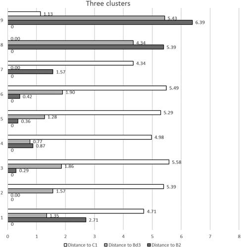
The distances from the polygons to the three cluster centers are illustrated with the data for 26th May (Figure 6). The three horizontal bars for each polygon show its remoteness along the x –axis in relation to the central polygons in the three clusters. The smaller the difference was in relation to the center of a given cluster, the closer the given polygon was to its core. For a polygon which is a cluster center, the difference with this cluster is zero. The distances from the polygons to the centers of the three clusters in the multidimensional space reflected the degree of separation of the different types of polygons. With all the polygons, the distances to the center of their cluster were at least four times lower that the ones to the centers of the other clusters. On 26th May, the algorithm successfully determined three polygons of different types as cluster centers, and the distance between the centers of the organic and biodynamic groups was more than three times shorter than their distance to the conventional group.

Figure 6. Distances from the polygons to the centers of the three clusters, 26th May.

The close values between the organic and biodynamic polygons, as well as the established differences between the conventional polygons, give reasons for analyzing the possibilities of distinguishing when setting the option of two clusters. For the four observation dates, different polygons were identified for cluster centers: for 3rd April B3 and Bd1; for 26th May B4 and C1; for 17th June Bd1 and C1 and for 25th June Bd1 and C2 (Table 8). For April 3rd, the conventional polygons were recognized as organic, while for all other dates they were recognized correctly as conventional. The biodynamic polygons were recognized as organic for 26th May, while for 17th and 25th June organic polygons are recognized as biodynamic. The best separation between all polygons (with the lowest value of SSE) was observed in the data for 17th June. With the polygons of 17th June (Table 8), the algorithm indicated that the central polygons were No 8 (C1) and No 5 (Bd1). The situation was also similar for 26th May and 25th June.

Table 8. Distances from polygons to the centers of the two clusters.

N	Code	Original type	3rd April				26th May
			Cluster centers		Min	Recognized type	Cluster centers		Min	Recognized type
			B3	Bd1			B4	C1
1	B1	B	18.01	0.06	0.06	Bd	3.37	22.18	3.37	B
2	B2	B	0.50	14.19	0.50	B	0.77	29.07	0.77	B
3	B3	B	0.00	17.10	0.00	B	1.36	31.08	1.36	B
4	B4	B	6.42	2.68	2.68	Bd	0.00	24.77	0.00	B
5	Bd1	Bd	17.10	0.00	0.00	Bd	0.29	28.00	0.29	B
6	Bd2	Bd	6.24	3.04	3.04	Bd	1.57	30.12	1.57	B
7	Bd3	Bd	33.78	2.95	2.95	Bd	0.59	18.85	0.59	B
8	C1	C	7.85	46.47	7.85	B	24.77	0.00	0.00	C
9	C2	C	0.28	14.00	0.28	B	36.40	1.28	1.28	C
	SSE				17.36		SSE		9.23
N	Code	Original type	17th June				25th June
			Cluster centers		Min	Recognized type	Cluster centers		Min	Recognized type
			Bd1	C1			Bd1	C2
1	B1	B	0.33	42.41	0.33	Bd	0.13	18.15	0.13	Bd
2	B2	B	0.39	48.17	0.39	Bd	0.48	23.37	0.48	Bd
3	B3	B	0.57	49.09	0.57	Bd	0.41	23.79	0.41	Bd
4	B4	B	0.72	52.17	0.72	Bd	0.51	24.66	0.51	Bd
5	Bd1	Bd	0.00	41.16	0.00	Bd	0.00	19.30	0.00	Bd
6	Bd2	Bd	2.13	25.07	2.13	Bd	0.71	12.88	0.71	Bd
7	Bd3	Bd	0.11	40.85	0.11	Bd	0.79	12.66	0.79	Bd
8	C1	C	41.16	0.00	0.00	C	49.25	7.26	7.26	C
9	C2	C	23.45	2.85	2.85	C	19.30	0.00	0.00	C
	SSE				7.10		SSE		10.29

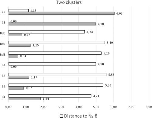
The distances from the polygons to the centers of the two clusters from the data for 26th May are presented in the diagrams in Figure 7. With all the polygons, the distances to the center of their cluster were at least nine times lower than the ones to the center of the other cluster.

Figure 7. Distances from the polygons to the centers of the two clusters, 26th May.

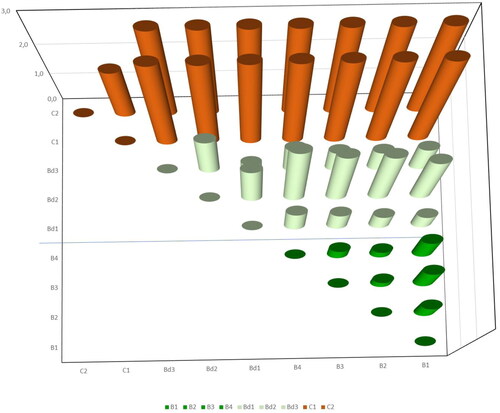
The polygons clustered in two groups, ‘all to all’, by dates, are illustrated with a 3 D diagram using the 17th June data, Figure 8. There the distance along the z-axis was measured in standard deviations. The group of organic polygons, at the bottom right, had low to medium values. With the rest of the dates, the separation was weakly expressed.

Figure 8. 3 D diagram of distances between polygons clustered into two groups, 17th June.

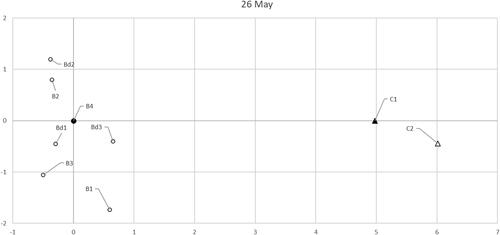
The distance in the 7-dimensional space between the two cluster centers and the position of the polygons which composed the clusters is shown in Figure 9. Each of the seven coordinate axes in this space is determined by one of the seven spectral indices used. The distances were calculated in standard deviations. On the plot diagrams for 26th May (Figure 9), the polygons were clearly divided into two clusters: conventional and mixed organic-biodynamic.

Figure 9. Plot of two clusters: ○ – member of cluster І, Δ – member of cluster ІІ, ▲● – cluster center.

Discussion

In situ observations of experimental fields reveal the presence of differences in the physiological and phеnological development of wheat plants from the same variety in the differently managed fields. Generally, the plant condition in the conventional and biodynamic fields was defined as better than in the organic one, based on intensity of the green color of leaves, plant height and percentage of projective cover of the aboveground plant parts. These differences in crop development are caused by the differences in the main agronomic practices applied in the studied fields. Although almost the same practices were applied in the organic and biodynamic fields (Table 2), the condition of wheat crops in them differed partly due to manure and biodynamic preparations applied in the biodynamic field and the resulting better nitrogen nutrition of biodynamic plants.

To be able to trace the differences noted above with remote methods, it is necessary to determine the spectral indices of the crops in the three types of fields. For this purpose in our study were used 10-meter resolution channels from Sentinel 2. This spatial pixel resolution proved to be detailed enough to conduct further procedures in distinguishing organic, biodynamic and conventional areas with winter wheat by means of multispectral images from satellite image data. Our findings also support a previous report [24] on wheat and cotton areas in Greece investigated by means of pictures from Sentinel-2 with 10-meter pixel resolution and WorldView-2 with 2-meter pixel. The authors established that the results for spectral indices NDVI and LAI (Leaf Area Index) obtained with the two types of sensors were comparable and that 10-meter pixels have a sufficiently high information potential [24].

Interpretation of individual index results

The polygons of 3rd April did not form groups for any of the seven indices, which can correspond to the organic, biodynamic and conventional. Two of the organic polygons showed deviation: B2 and B3. In all indices, they were closer to the conventional polygons than to the other two organic and biodynamic ones. In the drone picture with B2 and B3 there were spots of incomplete crop sowing. Therefore, their spectral characteristics were closer to the conventional polygons affected by winter drought.

With the polygons for 26th May, four indices (PSSRa, PSSRc, WDRVI, NDWI) formed two clearly distinguished groups: conventional and mixed organic-biodynamic (Figure 4). With two indices (NDVI and MSAVI), the above two groups were also well distinguished. Even though B1 had the opposite sign to the polygons in the organic-biodynamic group, it was clearly distinguished from the conventional by its tenfold lower values. Only with one index (CRI1) there was no distinction between the two groups. Deviation was observed in two of the organic polygons: B2 and B3. In all the indices, they were closer to the conventional polygons than to the other two organic and the biodynamic ones. The reasons for this have already been described above in the interpretation of the results of 3rd April.

With the polygons of 17th June two indices (CRI1 and PSSRc) formed two clear groups: conventional and mixed organic-biodynamic. With five of the indices (NDVI, PSSRa, WDRVI MSAVI and NDWI), the above two groups were also well distinguished, with Bd2 having the opposite sign than the polygons in the organic-biodynamic group, even though its values were close to theirs, and it was clearly distinguished from the conventional by its tenfold lower values. The aberrant Bd2 had the lowest crop density compared to the other two biodynamic polygons.

With the polygons for 25th June, six of the indices formed two clearly distinguished groups: conventional and mixed organic-biodynamic. With NDWI, the above two groups were also well distinguished; even though Bd3 had an opposite sign than the polygons in the organic-biodynamic group, it was clearly distinguished by its tenfold lower values. The aberrant Bd3 had an optimal crop density compared to the other two biodynamic polygons.

Generally, the results from the obtained spectral indices reflected the differences in the physiological state of the crops in both the different periods of their development and the differences in their condition depending on the type of cultivation.

Interpretation of clustering results

The obtained results of the clustering of the target polygons depend on the number of postulated groups and the dates of observation. By postulating 3 groups corresponding to three observed fields for three of the dates (3rd April, 17th June and 25th June) the algorithm specified two conventional polygons as cluster centers, which did not allow successful separation. For 26th May, the algorithm determined three polygons of different types as cluster centers (Figure 6), and the distance between the centers of the organic and biodynamic groups was more than three times shorter than their distance to the conventional group. The distances from the polygons to the centers of the three clusters in the multidimensional space reflected the degree of separation of the different types of polygons. With all the polygons, the distances to the center of their cluster were at least four times lower that the ones to the centers of the other clusters.

The sum of square standard deviations from the mean for each cluster, the Sum of Squared Errors (SSE), can be used as a measure for distinguishing between the three clusters in the 7-dimensional space. In an ideal theoretical case of complete separation, all the values of a cluster would coincide with the cluster center and the centers themselves would be far enough apart. Then SSE = 0, and in case of minimal deviations it tends to zero. Since SSE is essentially a sum, it depends on the number of elements, and in this case on the number of polygons − 9. When the mean value of standard polygon deviation is equal to ½ of the standard deviation, then SSE= 2.25. The final value of SSE= 4.08 obtained for 26th May showed good separation between the observed conventional, organic and biodynamic fields.

By postulating two clusters the best separation (with the lowest value of SSE) was observed in the data for 17th June, when all three groups of polygons (organic, biodynamic and conventional) were distinguished and each of them was differentiated on the plot in its own subgroup, although there were only two centers. The distances in standard deviations between the polygons for two clusters showed the best distinction of the three groups (Figure 8). The ‘error’ in distinguishing between organic and biodynamic polygons for three of the dates, 26th May, 17th June and 25th June, was a direct consequence of the presentation of three source polygon groups in two clusters (Table 8). The first date of observation, 3rd April, was not appropriate for successful separation between target polygons, because the algorithm specified one organic and one biodynamic polygon as cluster centers.

Under the specific unfavorable conditions until April, which gave priority to the wheat plants in the organic and biodynamic fields, the task of separating the polygons by types was further complicated. The faster and successful crop development in the conventional field, which was expected under favorable conditions, did not occur fully after the dry winter. This gave reason to assume that to establish the differences due to the type of agriculture, one should take into account the different conditions in the years, and comparison between the different types of polygons is best to be conducted only when a year has passed. Probably, after creating a sufficiently complete geo database for years of various conditions, one could search for and determine the interval in which the conditions can be considered as close enough to compare different types of polygons from different years with similar conditions.

The results presented here, though less categorical, are in line with those of other authors [17], showing that both spectral and spatial heterogeneity indices derived from multispectral satellite imagery enabled very efficient to full discrimination between organic and conventional maize fields.

Finally, the results from this pilot study give reasons for further research, where the scheme of the field experiment should be expanded and detailed in order to obtain a wider range of data. Then it will be possible to make a more comprehensive assessment of the algorithm developed so far and the perspectives for its application in practice.

Conclusions

The preliminary data from the approach used to distinguish conventional, organic and biodynamic fields of winter wheat showed that the approach was successful. The preliminary results from the analysis of the spectral indices showed that the differences in dynamics and development during the different growth and development stages of the crops in the organic, biodynamic and conventional fields can be traced by spectral characteristics from satellite images and they can be used to distinguish them. The success and degree of distinction depend on: the correct choice of multispectral satellite images in terms of spatial resolution (10 m pixel); the data from satellite images (spring-summer season) in the periods of tillering, earing, transition from milky ripeness to wax ripeness; the choice of suitable spectral indices (CRI 1, MSAVI, NDVI, NDWI, PSSR_a, PSSR_c, WDRVI); and the choice of analytical apparatus (multidimensional clusterization depending on the number of used indices). When setting future experimental areas, the efforts should be focused on providing more experimental areas of each type with similar environmental conditions.

Abbreviations
ATSAVI	=	adjusted transformed soil-adjusted vegetation index
NDVI	=	normalized difference vegetation index
CRI1	=	carotenoid reflectance index
NDWI	=	normalized difference water index
PSSRa	=	pigment specific simple ratio-Chla
PSSRc	=	pigment-specific simple ratio
MSAVI	=	modified soil adjusted vegetation index
WDRVI	=	wide dynamic range vegetation index

Disclosure statement

No potential conflict of interest was reported by the authors.

Additional information

Funding

This work was supported by the Bulgarian Ministry of Education and Science under the National Research Programme ‘Healthy Foods for a Strong Bio-Economy and Quality of Life’ approved by DCM # 557/17.08.2018. Framework Programme 2.1 ‘Food systems based on modern digital management methods,’ Task 2.1.1. Algorithms for distinguishing conventionally and organically grown crops using field survey data, drone aerial photographs and satellite images from Sentinel 2.

Notes

1 Biodynamics is a holistic approach to organic agriculture and horticulture, rooted in the work of Dr. Rudolf Steiner [18]. The application of biodynamic preparations (Bio 500-507), which are the foundation of biodynamics, revitalizes the soil, strengthens the plants and guides the fermentation processes in liquid fertilizers and compost heaps. This provides a possibility for optimal, balanced absorption of nutrients by plants and animals, which leads to stress reduction, harmonization of plant processes, resistance to pests and diseases and high-quality products. The application is performed in accordance with the planetary (lunar and terrestrial) position. Biodynamic agriculture has all possible beneficial effects on plants and soil: from improving soil properties, water, air circulation, to quality growth of plants and yield [19].

References

- Gerstmann H, Möller M, Gläßer C. Optimization of spectral indices and long-term separability analysis for classification of cereal crops using multi-spectral Rapid Eye imagery. Int J Appl Observ Geoinform. 2016; 52:115–125.
- Immitzer M, Vuolo F, Atzberger C. First experience with Sentinel-2 data for Cropand tree species classifications in Central Europe. RemoteSens. 2016; 8:166.
- Wei M, Qiao B, Zhao J, et al. The area extraction of winter wheat in mixed planting area based on Sentinel-2 a remote sensing satellite images. Int J Parallel Emergent Distrib Syst. 2019;
- Qi J, Chehbouni A, Huete AR, et al. A modified soil adjusted vegetation index. Remote Sens Environ. 1994;48(2):119–126.
- Rouse JW, Haas RH, Schell JA, et al. Monitoring the vernal advancements and retrogradation (green wave effect) of natural vegetation NASA, Greenbelt (MD): NASA/GSFC Final Report. 1974. p. 371.
- Martin MP, Barreto L, Fernandez-Quintanilla C. Discrimination of sterile oat (Avena sterilis) in winter barley (Hordeum vulgare) using Quick Bird satellite images. Crop Prot. 2011; 30issue (10):1363–1369.
- Riedell WE, Blackmer TM. Leaf reflectance spectra of cereal aphid-damaged wheat. Crop Sci. 1999;39(6):1835–1840. Npp
- Zheng Q, Huang W, Cui X, et al. New spectral index for detecting wheat yellow rust using Sentinel-2 multispectral imagery. Sensors. 2018;18(3):868.
- Babar MA, Reynolds MP, van Ginkel M, et al. Spectral reflectance to estimate genetic variation for in-season biomass, leaf chlorophyll, and canopy temperature in wheat. Crop Sci. 2006;46(3):1046–1057.
- Henrich V, Krauss G, Götze C, et al. IDB - www.indexdatabase.de, Entwicklung einer Datenbank für Fernerkundungsindizes. AK Fernerkundung, Bochum, 2012. 4, 5, 10. https://www.indexdatabase.de/db/s-single.php?id=96
- Blackburn GA. Spectral indices for estimating photosynthetic pigment concentrations: A test using senescent tree leaves. Int J Remote Sens . 1998;19(4):657–675.
- McFeeters SK. The use of the Normalized Difference Water Index (NDWI) in the delineation of open waterfeatures. Int. J. Remote Sens. 1996;17(7):1425–1432.
- Gitelson AA. Wide dynamic range vegetation index for remote quantification of biophysical characteristics of vegetation. J Plant Physiol. 2004; 161(2):165–173.
- Wu J, Wang D, Bauer ME. Assessing broadband vegetation indices and Quick Bird data in estimating leaf area index of corn and potato canopies. Field Crops Res. 2007;102(1):33–42.
- He Y, Guo X, Wilmshurst JF. Comparison of different methods for measuring leaf area index in a mixed grassland. Can J Plant Sci. 2007;87(4):803–813.
- Amujoyegbe BJ, Opabode JT, Olayinka A. Effect of organic and inorganic fertilizer on yield and chlorophyll content of maize (Zea mays L.) and sorghum (Sorghum bicolour (L.) Moench). Afr J Biotechnol. 2007;(6):1869–1873. http://doi.org/10.5897/AJB2007.000-2278
- Denis A, Desclee B, Migdall S, et al. Multispectral remote sensing as a tool to support organic crop certification: assessment of the discrimination level between organic and conventional maize. Remote Sens. 2020;13(1):117.
- Steiner R. Agriculture: A course of eight lectures. 3rd ed;London: Bio-Dynamic Agricultural Association, 1974.
- Diver S. Biodynamic Farming and Compost preparation. ATTRA, 1999. pp 20. http://citeseerx.ist.psu.edu/viewdoc/download?doi=10.1.1.405.2968&rep=rep1&type=pdf.
- Ninov N. Taxonomic list of soils in Bulgaria, according to the FAO World magazine. Teach Geograph. 2005;5 :4–18.
- Koteva V. Change in some parameters of soil fertility of the leached chernozem-smolnitza the influence of long-term mineral fertilization in crop rotation. [PhD Thesis]. Karnobat, 1993.
- Koteva V, Atanasova D. Soil analysis in the new field biological agriculture in the Agricultural Institute in Karnobat. In: International Scientific Conference Plant Genetic Stoks – the Basis of Agriculture of Today. 2007 June 13–14; Sadovo, Bulgaria, 2007. p. 687–688.
- Zarkov B, Penchev P. The Agro-meteorological conditions in the region of Karnobat in the 20th century. Plant Sci. 2000; 37:832–834.
- Psomiadis E, Dercas N, Dalezios NR, et al. Evaluation and cross-comparison of vegetation indices for crop monitoring from Sentinel-2 and WorldView-2 images. Proc. SPIE. 2017;10421:104211B..