A novel prediction method for protein DNA-binding residues based on neighboring residue correlations

Abstract

Accurately identifying the protein DNA-binding residues is important for understanding the protein–DNA recognition mechanism and protein function annotation. Many computational methods have been proposed to predict protein–DNA binding residues using protein sequence information; however, for severe imbalanced data like the protein–DNA binding dataset, the under-sampling technique which is applied by most previous methods cannot achieve satisfactory performance. In this study, an adjustment algorithm is proposed to offset the biased prediction results from the classifier. The proposed adjustment algorithm uses the binding probability between the target residue and its neighboring residues to identify more true binding residues which are wrongly predicted as non-binding. The proposed prediction method with adjustment algorithm achieves an area under the ROC curve (AUC) of 0.926 and 0.866 on two benchmark datasets and 0.882 on the independent testing set, which demonstrates that the proposed method can efficiently predict specific residues for protein–DNA interactions.

Keywords:

• Bioinformatics
• protein
• machine learning
• binding sites
• sequence information

Introduction

The interaction between protein and DNA is important for many essential biological processes such as DNA replication [1], repair [2] and modification processes [3]. Therefore, accurately identifying DNA-binding residues in protein sequences could lead to a better understanding for protein structure and functions. Many experimental approaches have been proposed for protein–DNA binding residue recognition, such as X-ray crystallography [4], nuclear magnetic resonance (NMR) spectroscopy [5], electrophoretic mobility shift assays (EMSAs) [6] and conventional chromatin immunoprecipitation (ChIP) [7]. However, these experimental methods often come along with time consumption and high economic costs which make them difficult for wide application [8]. Since there is an increasing number of protein sequences that have been detected by researchers, applying computational methods to predict protein DNA-binding residues is drawing more attention.

Many computational prediction methods have been proposed in recent years. According to the involved features, these prediction methods can be grouped into two categories: sequence information-based methods and structure information-based methods [9]. Before June 2021, the number of proteins with known structure in Protein Data Bank (PDB) [10] was about 1,78,451; whereas, the number of proteins with known sequence in Swiss-Prot Database [11] was about 5,64,638. The richer deposit number of protein sequences demonstrates that the prediction method based on protein sequence information has greater application prospects. In 2005, Ahmad et al. [12] proposed a neural network-based prediction method for protein–DNA binding residues, the Position Specific Scoring Matrix (PSSM), which was extracted from protein sequence alignments used as features. The prediction result showed that the evolutionary information in protein sequences was significant in the prediction of protein–DNA binding residues. Wang et al. [13] proposed BindN, which utilized the biochemical properties of amino acids such as the side-chain pKa value, hydrophobicity index and molecular mass as input features with Support Vector Machines (SVMs). Then, the evolutionary information was added into BindN to form BindN + [14], which showed better performance than the original BindN method. They also explored other classification algorithms for protein–DNA binding residues prediction and chose Random Forest (RF) to build BindN-RF [15] as another efficient prediction method. Ma et al. [16] developed DNABR, in which two types of sequence features were proposed. The first type of feature used evolutionary information combined with conservation of physicochemical properties, while the second type of feature reflected the dependency effect of amino acids in regard of polarity-charge and hydrophobic properties in protein sequences. Then the two types of features were sent into RF classifier to make prediction. In 2017, Zhou et al. [17] proposed a novel residue encoding method named PSSM-RT which utilized the relationships of evolutionary information between residues. To further improve the prediction performance, the ensemble learning algorithm was adopted which combined the results from SVM classifier and RF classifier for final prediction. In their work, they found that the binding probability of target residue could be affected by its adjacent residues on the left and right sides because some certain amino acids are important in the interaction between proteins and DNA molecules.

Although previous studies have made pioneering achievements for prediction of protein–DNA binding residues, the main improvements were made by using newly proposed classification algorithms. For the relationship between the binding properties and correlation of neighboring residues, corresponding research is still lacking, which leaves space for further improvements in prediction performance.

In this study, we proposed a sequence-based prediction method for protein–DNA binding residues. The evolutionary information and physicochemical properties of amino acids were adopted to form a feature matrix. LightGBM [18,19] was applied as a classifier; it is a novel Gradient Boosting Decision Tree (GBDT) [20] algorithm with gradient-based one-side sampling (GOSS) and exclusive feature bundling (EFB) to deal with big data and a large number of features. Compared with traditional classification algorithms such as SVM and RF, LightGBM shows faster training speed with a lower memory cost. The advantages of LightGBM make it suitable for high-throughput data tasks like analysis of protein sequences [21–23]. Inspired by Zhou et al. [17]’s study, we proposed an adjustment procedure based on residue neighboring correlation for the output of the LightGBM classifier. The prediction performance on the benchmark datasets over five-fold cross-validations and on the independent testing set demonstrates that our adjustment procedure could efficiently improve the prediction accuracy for protein–DNA binding residues in protein sequences. The source code and the benchmark datasets in this study can be freely accessed at https://github.com/tlsjz/DNAbinding.

Materials and methods

Datasets

To evaluate the performance of our proposed prediction method and to make comparison with other state-of-art prediction methods, two benchmark datasets and one independent testing set are used.

1. PDNA-62

   PDNA-62 [24] is a non-redundant dataset which contains 67 proteins from the Protein Data Bank (PDB). The CD-Hit [25] software is used to reduce the sequence pair-wise identity in PDNA-62 less than 25%. A residue is defined as DNA-binding if at least one of its atoms is less than 3.5 Å away from one atom in the DNA molecule. As a result, PDNA-62 contains 1215 DNA-binding residues and 6948 non-binding residues.

2. PDNA-224

   PDNA-224 [26] is another widely used non-redundant benchmark dataset for protein–DNA binding residues prediction which contains 224 protein sequences retrieved from the PDB database. The cut-off of sequence pair-wise identity is 25%. According to the identical criterion for the definition of DNA-binding residue in protein sequence, PDNA-224 contains 3778 binding residues and 53570 non-binding residues.

3. TS-72

To fully evaluate the generalization ability of our proposed method, an independent testing set is adopted. Ma et al. [16] extracted 337 DNA-interacting proteins from the PDB database with a structure resolution better than 3.5 Å. Redundant sequences were removed to keep the pair-wise identity lower than 25%. Among these sequences, 72 protein chains from 60 protein–DNA complexes were selected as a testing set named TS-72, the remaining 265 protein chains, referred to as TR-265, were used as a training set. As a result, the TR-265 training set contains 3818 binding residues and 50,993 non-binding residues, while the TS-72 testing set contains 1078 binding residues and 13,175 non-binding residues.

Feature extraction

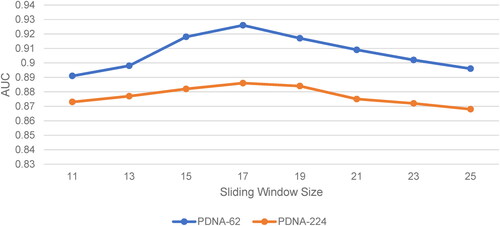
For prediction of protein–DNA binding residues, each data instance is obtained by a sliding window along the protein sequence. A sliding window of size L contains the feature of target residue in the middle and the features of (L-1)/2 adjacent residues on the left and right sides, respectively. For the selection of sliding window size, we tried to set L from 11 to 25. After calculation of corresponding performance under different sliding window sizes, we found that when L = 17, the classifier showed better performance. The prediction performance with different sliding window sizes for datasets PDNA-62 and PDNA-224 are shown in Figure 1. Therefore, the size of the sliding window was set to 17 in this study.

Figure 1. Prediction performance (AUC) using different sliding window sizes for PDNA-62 and PDNA-224 over five-fold cross-validations..

1. Position-specific scoring matrix (PSSM)

   For a given protein sequence, we generated the PSSM profile by running PSI-BLAST [27] against the non-redundant (nr) database with three iterations and an E-value of ${10}^{-3}$. The size of the PSSM profile is L*20 where L represents the length of protein sequence and 20 represents 20 types of amino acids in the protein sequence. Since the value in original PSSM is too sparse, we often normalized it to range of 0 and 1 with the following logistic function: (1) $$S_{i,r}^{\left(N\right)}=1/\left(1+e^{{-s}_{i,j}}\right)$$(1)

where $S_{i,r}^{(N)}$ represents the normalized value and $S_{i,j}$ represents the original value in the PSSM profile. For the sliding window of size 17, the dimension of PSSM feature was 17*20 = 340.

1. Predicted secondary structure

   Previous studies [17] have shown that protein secondary structure is relevant to protein–DNA binding properties. Protein secondary structures can be grouped into three types which are coil (C), helix (H) and strand (E)[28]. In this study, the PSIPRED [29] software was used to predict the secondary structure for the query sequences from the sequence information. Therefore, for the sliding window of size 17, the dimension of the predicted secondary structure feature was 17*3 = 51.

2. Residue one-hot encoding

   According to the dipoles and volumes of side chains of amino acids, 20 types of amino acids can be clustered into 7 classes as follows: Class A = {Ala, Gly, Val}, Class B = {Ile, Leu, The, Pro}, Class C = {His, Asn, Gln, Trp}, Class D = {Tyr, Met, Thr, Ser}, Class E = {Arg, Lys}, Class F = {Asp, Glu} and Class G = {Cys}[30]. Therefore, a 7-dimensional one-hot binary key was used to encode 20 types of amino acids. In the sliding window of size 17, the dimension of one-hot encoding feature was 17*7 = 119.

3. Residue physicochemical properties

Ten physicochemical properties of amino acids were considered in this study including the pKa values of amino groups, pKa values of carboxyl groups, side chain pKa values, electron-ion interaction potential (EIIP), molecular mass, hydrophobicity, hydrophilicity, polarity, polarizability and average accessible surface area. The value of each physicochemical property can be obtained from the AAindex [31] database. For a sliding window of size 17, the dimension of residue physicochemical properties feature was 17*10 = 170.

In summary, for each query residue, four types of sequence features were extracted: the PSSM feature, the predicted secondary structure feature, the residue one-hot encoding feature and the residue physicochemical property feature. The dimension of the feature matrix for each query residue was 340 (17*20) + 51 (17*3) + 119 (17*7) + 170 (17*10) = 680.

LightGBM classification algorithm

Gradient boosting decision tree (GBDT) is a widely used and efficient algorithm that can be used for both classification and regression problems [32–34] . In 2017, Ke et al. [19] proposed LightGBM, which can be considered as a fast and efficient type of GBDT. The LightGBM algorithm contains two novel techniques, which are the gradient-based one-side sampling (GOSS) and the exclusive feature bundling (EFB) to handle a large number of data instances and a large number of data features without overfitting problem, respectively.

When facing with high throughput data like protein sequences, LightGBM shows its advantage over other machine learning algorithms such as Support Vector Machines and Random Forests. The histogram algorithm applied by LightGBM converts the feature values into bins before training, and uses bins to index histograms instead of sorting the feature values, which greatly reduces the computation cost of split gain. Moreover, for the unbalanced data like protein DNA-binding residues, by setting the parameters, LightGBM gives a larger weight for the minority class during the training process, which helps to make the classifier focus more on the minority class instances. Therefore, in this paper, the LightGBM was chosen as the classification algorithm for the prediction.

Proposed N-stage adjustment procedure for outputs of LightGBM

Since each type of amino acid owns its specific physicochemical property, the DNA binding capability is varied for amino acids. The backbone of DNA is of negative polarity, which makes the amino acids with positive polarity more easily interact with DNA molecules. According to the definition of a DNA-binding residue, if the distance between the atoms in the amino acid and the DNA molecule is closer than the threshold, the amino acid will be identified as DNA-binding. The spatial arrangement of amino acids in a protein follows certain rules, therefore, if the neighboring residues are DNA-binding or have closer distance with DNA molecules, the target residue will have stronger DNA binding properties. We can name the binding propensity which is caused by the neighboring residues as residue neighboring correlation. Considering the unique physicochemical property of amino acids, the target residue has corresponding DNA-binding capabilities when it combines with different neighboring residues to form residue pairs. In fact, Zhou et al. [17] have referred to the correlation between DNA binding and residue pairs, however, they did not apply this correlation in their prediction method.

In this study, we proposed N-stage neighboring residue binding probability $P_{\mathit{NRB}-N}$. For residue $r1$ and $r2$, if residue $r1$ locates in the $i$th position in the protein sequence and residue $r2$ locates in the $(i+1)$th or ($i-1$)th position, they can be regarded as 1-stage neighboring; if residue $r2$ locates in the $(i+2$)th or ($i-2$)th position, they can be regarded as 2-stage neighboring; the higher stage neighboring can be defined in the same manner.

For the dataset with $L$ protein sequences, the N-stage neighboring binding probability for residue $r1$ and $r2$ can be obtained as follows: 1) For protein sequence $i$, $i=1,2,\dots ,L$, $S_{i(r1,r2)}^{\mathrm{\text{'}}}$ represents the frequency that residue $r1$ is DNA-binding when residue $r1$ and $r2$ are N-stage neighboring residues; $S_{i(r1,r2)}$ represents the frequency that residue $r1$ and $r2$ are N-stage neighboring residues. 2) Then the algorithm traverses the protein sequences in the dataset, and calculate $S_{(r1,r2)}^{\mathrm{\text{'}}}$ and $S_{(r1,r2)}$ of the dataset as follows: (2) $$S_{(r1,r2)}^{\mathrm{\text{'}}}={\sum }_{i=1}^L{S}_{i(r1,r2)}^{\mathrm{\text{'}}}$$(2) (3) $$S_{(r1,r2)}=\mathrm{ }{\sum }_{i=1}^L{S}_{i(r1,r2)}$$(3)

3) Next, we apply formula (4) to calculate the N-stage neighboring binding probability for residue $r1$ and $r2$ in the dataset. (4) $$P_{\mathit{NRB}-N}\left(r1,r2\right)=\frac{S_{(r1,r2)}^{\mathrm{\text{'}}}}{S_{(r1,r2)}}$$(4)

$P_{\mathit{NRB}-N}\left(r1,r2\right)$ represents the prior probability that $r1$ is DNA-binding when $r1$ and $r2$ are N-stage neighboring residues. For residue $r1$, its N-stage neighboring binding probability $P_{\mathit{NRB}-N}\left(r1\right)$ has 20 values which correspond to 20 types of amino acids in the protein sequence. Higher $P_{\mathit{NRB}-N}\left(r1,r2\right)$ means that residue $r1$ has stronger DNA binding capability when residue $r2$ occurs as the N-stage neighboring of $r1$.

Because of the severe data imbalance in the protein DNA-binding datasets, the original prediction results from classifier will be inevitably biased to the majority class. For protein–DNA binding residues prediction in which the number of non-binding residues is much larger than the number of binding residues, many true binding residues will be wrongly predicted as non-binding by the classifier. In order to offset the biased original prediction result, in this study, an adjustment algorithm was proposed for the outputs of classifier based on the correlation of neighboring residues.

The proposed adjustment algorithm can be summarized as follows:

1. For target residue $i$, if its original classification probability $P_{\mathit{original}}\left(i\right)$ is lower than the classification threshold, which means it is classified as non-binding by the classifier, the following adjustment procedure will be applied.

2. According to the 1-stage neighboring binding probability between the target residue and its 1-stage neighboring residue $P_{\mathit{NRB}-1}\left(i,i-1\right)$ and $P_{\mathit{NRB}-1}\left(i,i+1\right)$, we calculate the 1-stage adjusted classification probability $P_{1-\mathit{StagePrediction}}\left(i\right)$ as follows: (5) $$P_{1-\mathit{StagePrediction}}\left(i\right)=\{\begin{array}{c}{P}_{\mathit{original}}\left(i\right)+P_{\mathit{NRB}-1}\left(i,i-1\right)\times P_{\mathit{original}}\left(i-1\right) if{\mathrm{ }P}_{\mathit{NRB}-1}\left(\mathrm{i},i-1\right)>1-\mathit{StageThreshold}\\ P_{\mathit{original}}\left(i\right)+P_{\mathit{NRB}-1}\left(i,i+1\right)\times P_{\mathit{original}}\left(i+1\right) if{\mathrm{ }P}_{\mathit{NRB}-1}\left(i,i+1\right)>1-\mathit{StageThreshold}\end{array}$$(5)

3. Based on the 2-stage neighboring binding probability between the target residue and its 2-stage neighboring residue $P_{\mathit{NRB}-1}\left(i,i-2\right)$ and $P_{\mathit{NRB}-1}\left(i,i+2\right)$, we further adjust the classification probability of target residue to obtain the 2-stage adjusted classification probability $P_{2-\mathit{StagePrediction}}\left(i\right)$: (6) $$P_{2-\mathit{StagePrediction}}\left(i\right)=\{\begin{array}{c}{P}_{1-\mathit{StagePrediction}}\left(i\right)+P_{\mathit{NRB}-2}\left(i,i-2\right)\times P_{\mathit{original}}\left(i-2\right) if{\mathrm{ }P}_{\mathit{NRB}-2}\left(i,i-2\right)>2-\mathit{StageThreshold}\\ P_{1-\mathit{StagePrediction}}\left(i\right)+P_{\mathit{NRB}-2}\left(i,i+2\right)\times P_{\mathit{original}}\left(i+2\right) if{\mathrm{ }P}_{\mathit{NRB}-2}\left(i,i+2\right)>2-\mathit{StageThreshold}\end{array}$$(6)

It is worth mentioning that, if the proposed adjustment algorithm is used for all predicted non-binding residues, some true non-binding residues will be affected. Therefore, a threshold is set for the adjustment algorithm, and only if the $P_{\mathit{NRB}-N}\left(i,i-N\right)$ is larger than the threshold, will the adjustment algorithm be applied. The value of the threshold needs to be determined by experimental attempts; the detailed process will be discussed in the Results and Discussion section.

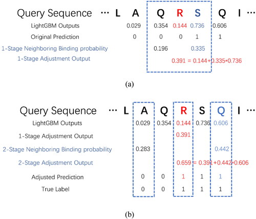
Figure 2 shows an application example of the proposed adjustment algorithm. The original classification probability of the target residue is 0.144, which is lower than classification threshold. In Figure 2(a), according to prior knowledge, the 1-stage neighboring binding probability between the target residue and its 1-stage neighboring $P_{\mathit{NRB}-1}\left(R,S\right)$ is 0.335. The 1-stage adjusted classification probability $P_{1-\mathit{StagePrediction}}\left(i\right)$ can be calculated using formula (5), $P_{1-\mathit{StagePrediction}}\left(i\right)=0.144+0.335\mathrm{*}0.736=0.391$. In Figure 2(b), the 2-stage adjusted classification probability can be obtained using formula (6), $P_{2-\mathit{StagePrediction}}\left(i\right)=0.391+0.442\mathrm{*}0.606=0.659$. After using the adjustment algorithm, the classification probability of the target residue is larger than the threshold; therefore, the target residue can be classified as DNA-binding, which coincides with its true label.

Figure 2. An example of proposed 1-stage adjustment algorithm (a) and 2-stage adjustment algorithm (b).

In this study, only 1-stage adjustment algorithm and 2-stage adjustment algorithm were adopted. We tried to apply a higher stage adjustment algorithm in the prediction method; however, it would lead to more false positive samples in the prediction result. The experimental results are displayed in Results and Discussion section. The detailed steps of the proposed adjustment procedure are shown in Algorithm 1.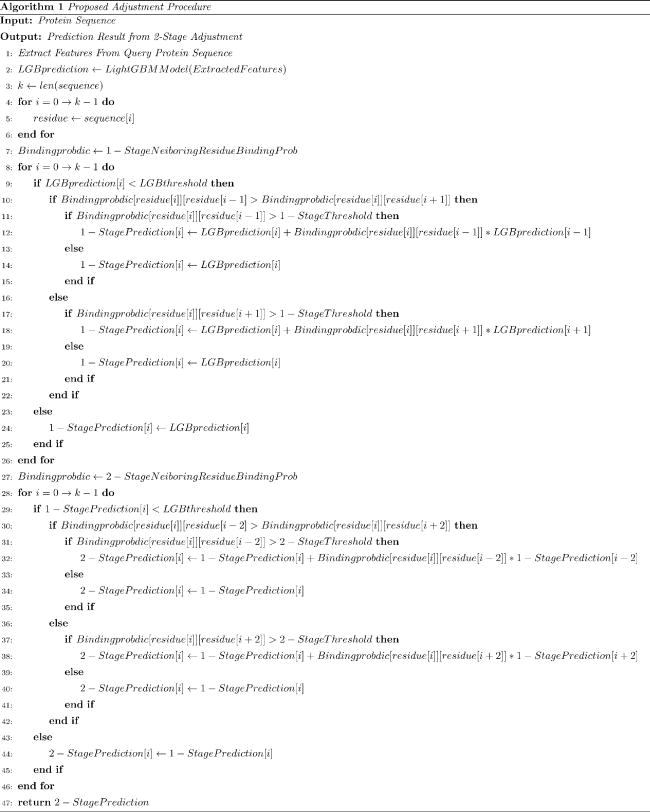

Performance evaluation

In this study, four routinely used evaluation criteria are applied to reveal the overall performance of the proposed prediction method including the overall accuracy (ACC), sensitivity (Sen), specificity (Spe) and Matthews Correlation Coefficient (MCC). The definitions of these criteria are shown below: (7) $$\mathit{ACC}=\mathrm{ }\frac{TP+TN}{TP+TN+FP+FN}$$(7) (8) $$\mathit{Sensitivity}=\mathrm{ }\frac{TP}{TP+FN}$$(8) (9) $$\mathit{Specificity}=\mathrm{ }\frac{TN}{TN+FP}$$(9) (10) $$\mathit{MCC}=\mathrm{ }\frac{TP\mathrm{*}TN-FP\mathrm{*}FN}{\sqrt{(TP+FP)(TP+FN)(TP+FP)(TN+FN)}}$$(10) where TP, TN, FP, FN represent the number of true positive instances, true negative instances, false positive instances and false negative instances in the prediction result, respectively.

Moreover, in the situation where severe imbalance exists in the benchmark dataset, the threshold-dependent criteria sometimes cannot objectively report the performance as they are largely affected by the ration of positive and negative instances in the dataset. Therefore, the Receiver Operating Characteristic (ROC) [35] curve is introduced. The x-axis and y-axis of ROC are the false positive rate (FPR) and true positive rate (TPR), respectively. One point in the ROC curve represents the classification performance under a certain threshold. By changing the classification thresholds, a curve can be drawn. Although the ROC curve can visually reveal the classification performance, the researchers still need to compare the performance numerically between classifiers. Consequently, the criterion, area under ROC curve (AUC), is developed. The value of AUC is usually located between 0.5 to 1.0, the AUC of 0.5 indicates a random classification performance and the AUC of 1.0 indicates the best classification performance. Since AUC is threshold-independent, a prediction method with a larger AUC value means it shows more stable and outstanding performance.

It is worth mentioning that we introduced five evaluation metrics in this study; however, since the sensitivity only concerns the accuracy of positive instances, and the specificity only concerns the accuracy of negative instances, they cannot fully reveal the overall performance of the classifier. For example, a classifier with high sensitivity and low specificity does not guarantee satisfactory overall performance, because it may tend to predict each instance as positive. Therefore, in the field of protein–DNA binding residues prediction, we mainly focus on the metrics of MCC and AUC, which directly indicates the overall performance of the prediction methods.

Results and discussion

Feature effectiveness analysis

In this study, four types of features are extracted from protein sequence including evolutionary residue conservation (ERC), predicted secondary structure (PSS), residue one-hot encoding (One-hot Encoding) and residue physicochemical property (PP). In order to validate the effectiveness of involved features, we compared the performance of classifiers constructed with individual features and different feature combinations. The prediction performance on PDNA-62 and PDNA-224 over five-fold cross-validations are listed in Table 1.

Table 1. Prediction performance of individual feature and different feature combinations on PDNA-62 and PDNA-224 over five-fold cross-validations.

Dataset	Involved feature	ACC	Sen	Spe	MCC	AUC
PDNA-62	ERC	0.887	0.432	0.953	0.434	0.841
	PSS	0.838	0.436	0.896	0.313	0.746
	One-hot Encoding	0.815	0.490	0.862	0.304	0.754
	PP	0.838	0.509	0.885	0.354	0.786
	ERC + PSS	0.895	0.364	0.972	0.438	0.845
	ERC + One-hot Encoding	0.852	0.621	0.885	0.440	0.849
	ERC + PP	0.895	0.417	0.964	0.459	0.872
	ERC + PSS + One-hot Encoding	0.863	0.439	0.952	0.446	0.872
	ERC + PSS + PP	0.889	0.397	0.970	0.449	0.876
	ERC + One-hot Encoding + PP	0.878	0.493	0.943	0.462	0.881
	All Feature	0.885	0.522	0.939	0.481	0.884
PDNA-224	ERC	0.831	0.593	0.849	0.294	0.812
	PSS	0.714	0.517	0.729	0.138	0.673
	One-hot Encoding	0.723	0.620	0.731	0.197	0.728
	PP	0.858	0.388	0.894	0.217	0.762
	ERC + PSS	0.887	0.458	0.919	0.312	0.817
	ERC + One-hot Encoding	0.892	0.448	0.926	0.319	0.823
	ERC + PP	0.875	0.523	0.901	0.323	0.826
	ERC + PSS + One-hot Encoding	0.890	0.452	0.922	0.324	0.828
	ERC + PSS + PP	0.886	0.467	0.915	0.327	0.829
	ERC + One-hot Encoding + PP	0.889	0.463	0.919	0.331	0.832
	All Feature	0.899	0.421	0.938	0.336	0.837

Note: ACC, overall accuracy; Sen, sensitivity; Spe, specificity; MCC, Matthews correlation coefficient.

When using individual features, the evolutionary residue conservation showed better performance than the other three features, the corresponding classifier achieved MCC of 0.434 and 0.294, AUC of 0.841 and 0.812 on PDNA-62 and PDNA-224, respectively. It demonstrates that evolutionary residue conservation is significant in the identification of DNA-binding residues. In other words, DNA-binding residues are important for protein functions, which makes them conserved in the course of evolution.

For feature combinations, since evolutionary residue conservation is indispensable for classifier construction, we regard it as a base feature to combine with other features. In two-feature combinations, the classifier with evolutionary residue conservation and residue physicochemical property achieved better performance with MCC of 0.459 and 0.323, AUC of 0.872 and 0.826 on the two datasets. In three-feature combinations, the combination of evolutionary residue conservation, residue one-hot encoding and residue physicochemical property had better MCC of 0.462 and 0.331, and better AUC of 0.881 and 0.832. Finally, when four features were adopted, the classifier achieved MCC of 0.481 and 0.336, AUC of 0.884 and 0.837 on PDNA-62 and PDNA-224 respectively, which surpassed the classifier constructed with individual feature and other feature combinations. The performance comparison indicates that all four features applied in this study are effective for prediction of protein–DNA binding residues, so removing any of the features will have a negative effect on the final prediction performance.

Performance evaluation of proposed adjustment algorithm

In Zhou et al. [17]’s study, they found that the pair-relationships between some residues are important to protein–DNA binding. Inspired by their finding, in this study, the N-stage neighboring residue binding probability $P_{\mathit{NRB}-N}$ was proposed to reveal the relationship between the correlation of neighboring residues and DNA–binding property. Higher $P_{\mathit{NRB}-N}$ indicates the combination of target residue and its N-stage neighboring residue is more significant for protein–DNA binding. To show the discriminative ability of the proposed neighboring residue binding probability, we drew the heatmap of $P_{\mathit{NRB}-1}$ from PDNA-62 and PDNA-224 in Figure 3 (a) and (b).

Figure 3. Heatmap of $P_{\mathit{NRB}-1}$ of PDNA-62 (a) and PDNA-224 (b).

Note: The x-axis and y-axis denote the 20 amino acid types, and every element denotes a specific $P_{\mathit{NRB}-1}(x,y)$.

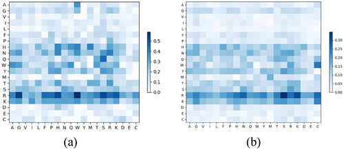
For both PDNA-62 and PDNA-224, the values of $P_{\mathit{NRB}-1}(R,G)$, $P_{\mathit{NRB}-1}(R,H)$, $P_{\mathit{NRB}-1}(R,W)$, $P_{\mathit{NRB}-1}(R,S)$, $P_{\mathit{NRB}-1}(R,K)$, $P_{\mathit{NRB}-1}(K,S)$, $P_{\mathit{NRB}-1}(K,K)$, $P_{\mathit{NRB}-1}(K,C)$, $P_{\mathit{NRB}-1}(Q,R)$ and $P_{\mathit{NRB}-1}(R,C)$ were larger than those of other residue pairs, which means they were easier to bind with DNA molecules in a protein–DNA complex. Noteworthily, the discriminative situation of $P_{\mathit{NRB}-2}$ was similar to $P_{\mathit{NRB}-1}$ on both PDNA-62 and PDNA-224.

After getting $P_{\mathit{NRB}-N}$, the proposed adjustment algorithm was applied for the outputs from the LightGBM classifier to offset the biased prediction results. In this study, the 1-stage adjustment algorithm and 2-stage adjustment algorithm were adopted. We also explored the performance of using higher stage adjustment algorithm. The results are shown in Table 2.

Table 2. Prediction performance of original LightGBM outputs, 1-stage adjustment, 2-stage adjustment and higher stage adjustment algorithm on PDNA-62 and PDNA-224 over five-fold cross-validations.

Dataset	Method	Acc	Sen	Spe	MCC	AUC
PDNA-62	0-stage (original LightGBM outputs)	0.885	0.522	0.939	0.481	0.884
	1-stage	0.870	0.671	0.913	0.572	0.917
	1-stage + 2-stage	0.875	0.736	0.895	0.590	0.926
	1-stage + 2stage + 3stage	0.862	0.801	0.873	0.581	0.920
	1-srage + 2-stage + 3-stage + 4-stage	0.851	0.821	0.856	0.570	0.915
PDNA-224	0-stage (original LightGBM outputs)	0.899	0.421	0.938	0.336	0.837
	1-stage	0.889	0.541	0.916	0.359	0.861
	1-stage + 2-stage	0.878	0.558	0.904	0.371	0.866
	1-stage + 2stage + 3stage	0.866	0.591	0.886	0.356	0.862
	1-srage + 2-stage + 3-stage + 4-stage	0.858	0.621	0.876	0.349	0.859

Note: ACC, overall accuracy; Sen, sensitivity; Spe, specificity; MCC, Matthews correlation coefficient.

The best performance was achieved when using the 1-stage adjustment algorithm and 2-stage adjustment algorithm for both PDNA-62 and PDNA-224. When the adjustment algorithm was not adopted, the prediction result was the original outputs from the LightGBM classifier, the sensitivity of the prediction result was relatively low, which indicates that many true binding residues were not correctly predicted and the classifier was biased to non-binding class. After the 1-stage and 2-stage adjustment algorithms were applied, the sensitivity improved even though the specificity had a little decline because when the wrongly predicted true binding residues were adjusted, some true non-binding residues were inevitably affected by the adjustment algorithm. However, the prediction still achieved the best overall performance with MCC of 0.590 and AUC of 0.926 for PDNA-62 and MCC of 0.371 and AUC of 0.866 for PDNA-224. When the higher stage adjustment algorithm was used for prediction, although the sensitivity was further improved, the specificity continued to decline at the same time. The overall performance decreased because more true non-binding residues were wrongly predicted by the adjustment algorithm. Therefore, in this study, the 1-stage adjustment algorithm and 2-stage adjustment algorithm were adopted, since they achieved the best overall performance in the prediction results.

Threshold selection for adjustment algorithm

In this study, we proposed the neighboring residue binding probability $P_{\mathit{NRB}-N}$ to show the DNA binding property of neighboring residues depending on the type of amino acids. Then we proposed an adjustment algorithm aiming at the predicted non-binding residues to offset the biased prediction results from the classifier trained on an imbalanced dataset. However, if we used the adjustment algorithm on each predicted non-binding residue, it would not only cost more time consumption in prediction process, but also would make more true non-binding residues wrongly predicted. Therefore, a threshold should be set for the adjustment algorithm: the N-stage adjustment algorithm would be applied only if the $P_{\mathit{NRB}-N}$ was larger than the N-stage threshold. We tried different thresholds from 0.1 to 0.9 for the 1-stage and 2-stage adjustment algorithm on PDNA-62 and PDNA-224 over five-fold cross-validations. The corresponding AUC values are listed in Figure 4. We first set the step of 0.1 in the range of 0.1 to 0.9 to roughly find the optimal range, then we set the step of 0.01 to find the exact threshold in the optimal range. For example, for the 1-stage threshold in PDNA-62, the optimal range was 0.2 to 0.3, and the exact threshold was 0.28 which corresponded to the highest AUC value.

Figure 4. Threshold selection for 1-stage and 2-stage adjustment algorithm on PDNA-62 and PDNA-224 over five-fold cross-validations.

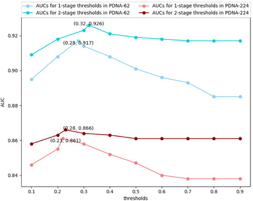
For the 1-stage adjustment algorithm, the best AUC was achieved when the threshold was set to 0.28 and 0.23 for PDNA-62 and PDNA-224, respectively. For the 2-stage adjustment algorithm, the best threshold should be set to 0.32 and 0.28 for PDNA-62 and PDNA-224, respectively. Moreover, we found from Figure 4 that the threshold for the 2-stage adjustment algorithm was larger than the threshold for the 1-stage adjustment algorithm. This could be explained by the correlation of 2-stage neighboring being less significant than the correlation of 1-stage neighboring; therefore, only when the target residue and its 2-stage neighboring residue have larger $P_{\mathit{NRB}-2}$, the 2-stage adjustment algorithm could be used to improve the overall performance.

Performance comparison with other prediction methods

In previous studies, many DNA-binding residues prediction methods were proposed which were trained and tested either on PDNA-62 or PDNA-224, such as Dps-pred[24], Dbs-pssm [12], BindN [13], Dp-bind [36], DP-Bind [37], BindN-RF [15], BindN+ [14], PreDNA [26] and EL_PSSM-RT [17]. It is worth mentioning that some of these methods were only trained and tested on PDNA-62, and others were trained and tested on both datasets. Since PreDNA used both sequential and structural information, in order to fairly compare with other methods, the version of PreDNA without using structural information was used in this study. Therefore, the prediction performance of our proposed method and other state-of-art methods are shown in Tables 3 and 4 for PDNA-62 and PDNA-224, respectively.

Table 3. Prediction performance of our proposed method and other state-of-art methods on PDNA-62 over five-fold cross-validations.

Method	Acc	Sen	Spe	MCC	AUC
Dps-pred	0.791	0.403	0.818	–	–
Dbs-pssm	0.664	0.682	0.660	–	–
BindN	0.703	0.694	0.705	-	0.752
Dp-bind	0.781	0.792	0.772	0.490	–
DP-Bind	0.772	0.764	0.766	–	–
BindN-RF	0.782	0.781	0.782	–	0.861
BindN+	0.790	0.773	0.793	0.440	0.859
PreDNA*	0.794	0.768	0.797	0.420	–
EL_PSSM-RT	0.808	0.850	0.801	0.510	0.901
Proposed Method	0.875	0.736	0.895	0.590	0.926

Note: ACC, overall accuracy; Sen, sensitivity; Spe, specificity; MCC, Matthews correlation coefficient.

* PreDNA without using structural information.

Table 4. Prediction performance of our proposed method and other state-of-art methods on PDNA-224 over five-fold cross-validations.

Method	Acc	Sen	Spe	MCC	AUC
PreDNA*	0.791	0.695	0.798	0.290	–
EL_PSSM-RT	0.781	0.796	0.780	0.340	0.865
Proposed Method	0.889	0.541	0.916	0.371	0.866

Note: ACC, overall accuracy; Sen, sensitivity; Spe, specificity; MCC, Matthews correlation coefficient.

* PreDNA without using structural information.

For PDNA-62, our method achieved the best MCC of 0.590 and AUC of 0.926, which are superior to other methods, especially for MCC, which reveals the performance in binary prediction. For PDNA-224, our method kept stable performance with MCC of 0.371 and AUC of 0.866, which outperformed other prediction methods. The results on both datasets indicated that our method with the adjustment algorithm had a discriminative ability for protein–DNA binding residues.

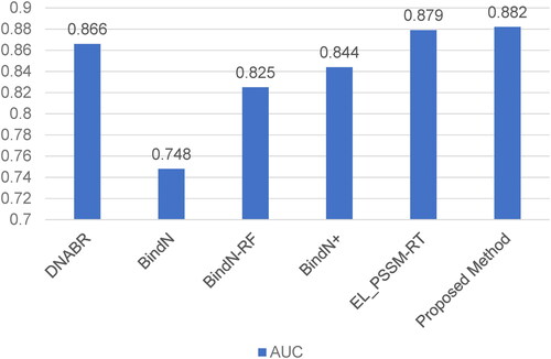
In order to further assess the proposed method, we compared our method with other methods on the independent testing set TS-72. Since previous studies only displayed the AUC value of TS-72, we showed the AUC comparison result in Figure 5. Our method achieved the best AUC of 0.882, which outperformed other methods by 0.003 to 0.134. The prediction result on the independent testing set demonstrated that our method had good generalization capability for protein–DNA binding residues.

Figure 5. AUC comparison between our proposed method and other prediction methods on the independent testing set TS-72.

Case study

In order to further evaluate the usefulness of the proposed adjustment algorithm, we displayed the prediction result of a protein–DNA complex, which was not included in the training set with PDB id of 3PVP_A. The original output from the LightGBM classifier, the prediction result of using the 1-stage adjustment algorithm and the prediction result of using the 1-stage and 2-stage adjustment algorithm are shown in Figure 6(a–(c).

Figure 6. The prediction result of 3PVP_A of original LightGBM outputs (a), 1-stage adjustment algorithm (b) and 1-stage and 2-stage adjustment algorithm (c). The green spheres, yellow spheres and red spheres denote the true positive (TP) instances, false negative (FN) instances and false positive (FP) instances, respectively.

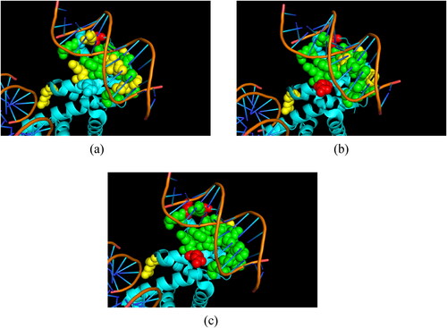
The prediction result of the original LightGBM classifier had 9 TP instances, 8 FN instances and 1 FP instances. After applying the 1-stage adjustment algorithm, the prediction result had 13 TP instances, 4 FN instances and 2 FP instances. The increased number of TP instances indicated that the adjustment algorithm could correct the wrongly-predicted true binding residues in the original LightGBM outputs. When using the 1-stage and 2-stage adjustment algorithm, the prediction performance was further improved with 15 TP instances, 2 FN instances and 3 FP instances. The MCC values for Figure 4(a)–(c) were 0.645, 0.777 and 0.826, respectively. The number of FP instances has a little increase after applying the proposed adjustment algorithm; however, the number of FN instances significantly declined and the overall performance improved at the same time. The prediction results on 3PVP_A demonstrated that the proposed adjustment algorithm could effectively identify more true binding residues for the biased results from the original classifier and correspondingly improve the overall performance.

Conclusions

The prediction of protein DNA-binding residues is a classic imbalanced learning problem, the number of non-binding residues is much larger than the number of binding residues. Therefore, the outputs of the classifier trained on imbalanced data are inevitably biased to the majority class. In order to offset this biased prediction results, in this study, an adjustment algorithm was proposed aiming at the predicted non-binding residues based on neighboring residue binding probability. The main purpose of the proposed adjustment algorithm is to correct these true binding residues which were wrongly predicted by the biased classifier. The prediction results on two benchmark datasets over five-fold cross-validations demonstrated that the proposed adjustment algorithm was effective to achieve better performance than other state-of-art sequence-based prediction methods. To further evaluate the algorithm, an independent testing set was used, and our proposed method achieved the best AUC value among the comparison methods. The satisfactory performance on the benchmark datasets and the independent testing set indicated that our proposed method showed competitive performance in identifying DNA-binding residues in proteins. Our study enriched the correlation between the residue binding property and residue pair-relationship which could be further adopted to other protein-ligands binding researches.

Acknowledgments

This work was supported by The National Nature Science Foundation of China (Grant Nos. 61972174,61662057 and 61772226), The Natural Science Foundation of Jilin Province (Grant number No. 20200201159JC), Key Laboratory for Symbol Computation and Knowledge Engineering of the National Education Ministry of China, Jilin University.

Disclosure statement

The authors declare no commercial or financial conflict of interest.

Data availability statement

The data that support the findings of this study are openly available at https://github.com/tlsjz/DNAbinding.

Additional information

Funding

This work was supported by The National Nature Science Foundation of China (Grant Nos. 61972174,61662057 and 61772226), The Natural Science Foundation of Jilin Province (Grant number No. 20200201159JC), Key Laboratory for Symbol Computation and Knowledge Engineering of the National Education Ministry of China, Jilin University.

References

- Pan Y, Zhou S, Guan J. Computationally identifying hot spots in protein-DNA binding interfaces using an ensemble approach. BMC Bioinf. 2020;21(Suppl 13):384.
- Biswas A, Narlikar L. Resolving diverse protein-DNA footprints from exonuclease-based ChIP experiments. Bioinformatics 2021;37(Supplement_1):i367–i375.
- Cozzolino F, Iacobucci I, Monaco B, et al. Protein-DNA/RNA interactions: an overview of investigation methods in the -omics era. J Proteome Res. 2021;20(6):3018–3030.
- Takaya D, Niwa H, Mikuni J, et al. Protein ligand interaction analysis against new CaMKK2 inhibitors by use of X-ray crystallography and the fragment molecular orbital (FMO) method. J Mol Graph Model. 2020;99:107599.
- Aihara H, Ito Y, Kurumizaka H, et al. The N-terminal domain of the human Rad51 protein binds DNA: structure and a DNA binding surface as revealed by NMR. J Mol Biol. 1999;290(2):495–504.
- Inoue N, Pellett PE. Human herpesvirus 6B origin-binding protein: DNA-binding domain and consensus binding sequence. J Virol. 1995;68(8):4619–4627.
- Kuhl AJ, Ross SM, Gaido KW. Using a comparative in vivo DNase I footprinting technique to analyze changes in protein-DNA interactions following phthalate exposure. J Biochem Mol Toxicol. 2007;21(5):312–322.
- Yang C, Ding Y, Meng Q, et al. Granular multiple kernel learning for identifying RNA-binding protein residues via integrating sequence and structure information. Neural Comput & Applic. 2021;33(17):11387–11399. doi:10.1007/s00521-020-05573-4.
- Ronesh S, Shiu K, Tatsuhiko T, et al. Single-stranded and double-stranded DNA-binding protein prediction using HMM profiles. Anal Biochem. 2021;612:113954. ISSN 0003-2697, https://doi.org/10.1016/j.ab.2020.113954.
- Berman HM, Westbrook J, Feng Z, et al. The protein data bank. Nucleic Acids Res. 2000;28(1):235–242.
- Bairoch A, Apweiler R. The swiss-prot protein sequence data bank and its new supplement TREMBLE. Nucleic Acids Res. 1996;21:21–25.
- Ahmad S, Sarai A. PSSM-based prediction of DNA binding sites in proteins. BMC Bioinf. 2005;6:33.
- Wang L, Brown SJ. BindN: a web-based tool for efficient prediction of DNA and RNA binding sites in amino acid sequences. Nucleic Acids Res. 2006;34:243–248.
- Wang L, Huang C, Yang MQ, et al. BindN + for accurate prediction of DNA and RNA-binding residues from protein sequence features. BMC Syst Biol. 2010;4(S1):S3.
- Wang L, Yang MQ, Yang JY. Prediction of DNA-binding residues from protein sequence information using random forests. BMC Genomics. 2009;10(Suppl 1):S1.
- Ma X, Guo J, Liu HD, et al. Sequence-based prediction of DNA-binding residues in proteins with conservation and correlation information. IEEE/ACM Trans Comput. Biol Bioinf. 2012;9(6):1766–1775.
- Zhou JY, Lu Q, Xu RF, et al. EL_PSSM-RT:DNA-binding residue prediction by integrating ensemble learning with PSSM relation transformation. BMC Bioinf. 2017;18(1):379.
- Liu Y, Yu Z, Chen C, et al. Prediction of protein crotonylation sites through LightGBM classifier based on SMOTE and elastic net. Anal Biochem. 2020;609:113903.
- Ke G, Meng Q, Finley T, et al. LightGBM: a highly efficient gradient boosting decision tree In Proceedings of the 31st Conference on Neural Information Processing System, Long Beach, CA, USA, p. 4–9. December 2017.
- Friedman JH. Greedy function approximation: a gradient boosting machine. Annals of Statistics. 2001;29(5):1189–1232.
- Chen C, Zhang Q, Ma Q, et al. LightGBM-PPI: Predicting protein-protein interactions through LightGBM with multi-information fusion. Chemometr Intell Lab Syst. 2019;191:54–64.
- Zhang L, Liu M, Qin X, et al. Succinylation site prediction based on protein sequences using the IFS-LightGBM (BO) model. Comput Math Methods Med. 2020;2020:8858489–8858415.
- Zhan ZH, You ZH, Li LP, et al. Accurate prediction of ncRNA-protein interactions from the integration of sequence and evolutionary information. Front Genet. 2018;9:458.
- Shandar A, Michael GM, Akinori S. Analysis and prediction of DNA-binding proteins and their binding residues based on composition, sequence and structural information. Bioinformatics 2004;20(4):477–486.
- Li W, Godzik A. Cd-hit: a fast program for clustering and comparing large sets of protein or nucleotide sequences. Bioinformatics 2006;22(13):1658–1659.
- Li T, Li Q-Z, Liu S, et al. PreDNA: accurate prediction of DNA-binding sites in proteins by integrating sequence and geometric structure information. Bioinformatics 2013;29(6):678–685.
- Altschul SF, Madden TL, Schäffer AA, et al. Gapped BLAST and PSI-BLAST: a new generation of protein database search programs. Nucleic Acids Res. 1997;25(17):3389–3402.
- Cuff JA, Barton GJ. Application of multiple sequence alignment profiles to improve protein secondary structure prediction. Proteins 2000;40(3):502–511.
- McGuffin LJ, Bryson K, Jones DT. The PSIPRED protein structure prediction server. Bioinformatics 2000;16(4):404–405.
- Wuthrich K, Billeter M, Braun W. Pseudo-structures for the 20 common amino acids for use in studies of protein conformations by measurements of intramolecular proton-proton distance constraints with nuclear magnetic resonance. J Mol Biol. 1983;169(4):949–961.
- Shuichi K, Minoru K. AAindex: Amino acid index database. Nucleic Acids Res. 1999;1:368–369.
- Pan Y, Liu D, Deng L. Accurate prediction of functional effects for variants by combining gradient tree boosting with optimal neighborhood properties. PLoS One. 2017;12(6):e0179314.
- Fan C, Liu D, Huang R, et al. Predrsa: a gradient boosted regression trees approach for predicting protein solvent accessibility. BMC Bioinf. 2016;17(S1):8.
- Liao Z, Wan S, He Y, et al. Classification of small gtpases with hybrid protein features and advanced machine learning techniques. CBIO 2018;13(5):492–500.
- Swets J. Measuring the accuracy of diagnostic system. Science 1988;240(4857):1285–1293.
- Shandar A, Michael GM, Akinori S. Analysis and prediction of DNA-binding proteins and their binding residues based on composition, sequence and structural information. Bioinformatics. 2004;20(4):477–486.
- Hwang S, Gou Z, Kuznetsov AIB. DP-Bind: a web server for sequence-based prediction of DNA-binding residues in DNA-binding proteins. Bioinformatics 2007;23(5):634–636.