Australian dams and reservoirs within a global setting

ABSTRACT

There has been a resurgence of interest in the construction of large dams worldwide. This study examined many dams from around the world (>10,000) and compared them to a comprehensive dataset developed for Australia (224) to provide insights that might otherwise not be apparent from examining just one or several dams. The dam datasets (ICOLD and ANCOLD) largely confirm existing narratives on Australian dam construction. Compared to dams from Rest of the World (RoW), Australian dams were found to:

• have larger reservoir capacities and spillway capacities for a given catchment area;

• have higher dam walls for a given capacity; and

• result in higher degrees of river regulation.

A range of general relationships among reservoir capacities, reservoir surface areas, and catchment areas are presented which can be used in reconnaissance or pre-feasibility studies and for global hydrologic modelling when dam and reservoir information are required as input.

KEYWORDS:

• Water resources
• ICOLD
• ANCOLD

1. Introduction

In recent years there has been a resurgence of interest in the construction of large dams in Australia and around the world. While across most of the rest of the world (RoW) the primary driver for dam development is hydroelectric power (Zarfl et al. 2015), in Australia the primary interest in the construction of new large dams is for supply of water for ‘greenfield’ irrigation in the relatively undeveloped northern half of Australia (DAWR 2016; PMC 2015; Petheram et al. 2014), and securing a reliable supply of water for regional cities and towns and existing irrigation areas.

During the second half of the twentieth century large dams in southern Australia have been effective in providing reliable water supplies in a dry and variable climate and have profoundly influenced the nation’s development by supplying 75% of Australia’s ~25,000 GL (gigalitre) (10 × 10⁶ m³) total annual water use (CSIRO 2011). However, these dams, mostly constructed in southern Australia between 1955 and 1980, have resulted in the regulation of flow in many of southern Australia’s rivers, in some cases contributing to complex and unpredictable environmental and social change. Prolonged dry periods in southern Australia in the early twenty-first century (i.e. 1996 to 2009; 2012 to 2015 and 2017 to 2019) have resulted in greatly reduced inflows to many reservoirs exacerbating conflict between upstream and downstream users and those advocating for the restoration of flows for the environment (e.g. The Conversation 2011). Consequently, the large, often public, capital expenditure and environmental and social changes have led some sectors of the public in Australia (e.g. O’Donnell and Hart 2016; Australian Geographic 2008) and globally (e.g. International Rivers 2015; WCD 2000) to question whether dams are an appropriate pathway for development.

For these reasons, the decision to construct a dam in Australia is more complex today than several decades ago. Despite there being vast quantities of literature on nearly all aspects of dams and reservoirs, limited attempts have been made to ‘mine’ large country (e.g. ANCOLD 2010) and global databases (e.g. ICOLD 2011) on dams for information to provide insights that might otherwise not be apparent from examining just one or several dams.

This is one of the two complementary papers that together deal with factors relating to the costs, sizing, and construction features of dams, spillways and outlet structures and related reservoir capacities. In this paper, we relate through graphical and statistical techniques dams, spillways, and reservoir physical features to at-site, catchment, and climate attributes for Australia and the RoW. In the companion paper (Petheram and McMahon 2019), costs for Australian dams are explored along with cost overruns, operation, and maintenance costs, and project features like the number of years to complete construction. In doing so, these two papers seek to contribute to better inform the debate and decision-making on dam development in Australia. The underlying premise driving this study is that understanding the history, the characteristics, and the global setting of Australian dams and related infrastructure better inform water resources engineering decision-making. To do this, we focus on the following three primary objectives:

1. To relate and substantiate general patterns and narratives of historical drivers of dam construction and design in Australia with empirical data (Section 3).

2. To examine the characteristics of Australian dams within a global context (Section 4 and 5).

3. To develop regression relationships that could inform pre-feasibility analysis of spillway capacity of potential dam sites, particularly in Australia, and provide guidance as to the utility of regionally based regression relationships elsewhere in the world, and which variables are likely to explain the most variance (Section 6).

Following this introduction, Section 2 describes the data used in the paper and their sources. Section 3 addresses the first objective by data mining the large dataset on dams in Australia within the context of the existing literature on dam construction. In Section 4 the two large datasets on dams in Australia and the Rest of the World are compared with specific reference to reservoir capacity, reservoir surface area, and catchment area. Spillways in Australia and RoW are compared in Section 5. Section 6 includes some summary comments, and key messages are provided in the concluding Section 7. The appendix material includes a list of symbols (Tables A1 and A2) and additional tables (Tables A3–A5) and figures (Figures A1 and A2), and Equations (A1(A1) $A=\frac{ab{h}^2}{2}$(A1) and A2(A2) $V=\frac{ab{h}^3}{6}$(A2) ) that explore the relationships between the physical features of Australian dams and reservoirs and catchment and climate attributes.

Table 1. Comparison for the period of 1850 − 2015 of the number (expressed as percentages) of the types of dam construction and year of dam completion in Australia (224 dams) with the rest of world (6944 dams)Multi-type dams are not considered for which there are 1637 in RoW.

Period	Aus or RoW	Barrage^b	Concrete buttress	Rock embankment	Multiple concrete arch	Concrete gravity	Earth embankment	Concrete arch	Total percent
1850–1869	Aus						0.45		0.45
	RoW						0.06		0.06
1870–1889	Aus						1.34		1.34
	RoW	0.01		0.01		0.09	0.28	0.01	0.40
1890-1909	Aus					1.34	1.79		3.13
	RoW			0.06		0.26	0.95	0.01	1.28
1910-1929	Aus			0.45		3.57	2.68		6.70
	RoW		0.22	0.13	0.06	1.97	2.62	0.27	5.27
1930–1949	Aus		0.89	0.45		1.34	1.78	1.79	6.25
	RoW	0.14	0.29	0.42	0.14	2.30	4.37	0.49	8.15
1950–1969	Aus		0.45	16.06		5.36	11.60	3.57	37.04
	RoW	0.26	1.14	2.45	0.17	3.30	20.49	1.92	29.73
1970–1989	Aus			19.20	0.45	5.36	10.71	0.89	36.61
	RoW	0.16	0.32	5.05	0.09	4.57	23.91	1.81	35.91
1990–2009	Aus			2.68		1.79	3.12		7.59
	RoW	0.10	0.12	3.44	0.06	3.01	7.24	1.47	15.44
2010–	Aus					0.89			0.89
	RoW	0.01		1.23	0.03	1.05	1.21	0.23	3.76
Total Percent^a	Aus		1.34	38.84	0.45	19.64	33.48	6.25
	RoW	0.68	2.09	12.79	0.55	16.55	61.11	6.21

^aRounding errors; ^bThis dam type category was not listed in the ANCOLD database.

Table 2. Purpose of reservoirs in Australia and in the rest of world.

Feature	Australia 224 reservoirs	Rest of world 7405 reservoirs
Flood control	1 (0.4%)	320 (4.3%)
Hydroelectric	40 (17.8%)	1851 (25.0%)
Irrigation	38 (16.9%)	2011 (27.2%)
Recreation	2 (0.9%)	245 (3.3%)
Water supply	84 (37.5%)	772 (10.4%)
Navigation	0 (0.0%)	58 (0.8%)
Multi-use	59 (26.3%)	2148 (29.0%)

Table 3. Dam site lithology, dam type, and height (224 Australian dams, 7795 RoW dams).

			Earth or rock dam		Concrete dam
Area	Lithology^a	Variables	Rock embankment	Earth embankment	Concrete buttress	Concrete arch	Multiple concrete arch	Concrete gravity
Australia	Unconsolidated sediments	Number (%) Median height (m) Range (m)	4.5 44 32–74	10.8 17 12–22	0	0	0	3.6 12 10–16
	Consolidated sediments	Number (%) Median height (m) Range (m)	16.7 55 43–74	13.5 36 24–46	1.4 34	3.6 55 49–83	0.5 38	5.9 45 38–57
	Hard rock	Number (%) Median height (m) Range (m)	18.0 47 30–68	9.5 32 24–46	0	1.8 42 38–67	0	10.4 41 33–50
RoW	No details available	Number (%) Median height Range (m)	13 56 37–87	60 29 20–41	2 41 22–61	6 65 47–91	1 44 26–86	19 44 27–65

^aConsolidated lithology at the dam wall derived from the Surface Geology of Australia 1:1 million scale dataset 2012 edition.

Table 4. Summary of key data for Australian and rest of world dams.

Variable	Number	Max.	25%’ile	Median	75%’ile	Min.
Australia
Catchment area (km^2)^1	176^a	113,879	1128	323	107	6.4
Annual catchment rainfall (mm/year)^2	176^a	3177	1355	977	792	221
Annual runoff (mm/year)^3	176^a	2490	464	182	93	5.1
Catchment aridity index^4	176^a	3.8	1.1	0.8	0.6	0.1
Reservoir yield (85% annual time-reliability) (ratio of mean annual flow)^5	169^a	1.10	0.85	0.75	0.58	0.14
Catchment elevation range (m)^1	176^a	2071	1014	601	341	12
Catchment slope mean (%)^1	176^a	19.6	11.8	6.9	4.3	0.8
Catchment woody raster (woody 1, non-woody 0)^6	176^a	1.00	0.99	0.80	0.51	0.00
Dam height (m)^7	217	180	55	42	24	7
Dam volume (10^3 m^3)^7	201	300,000	980	382	124	5
Reservoir capacity (10^6 m^3 or GL)^7	217	12,359	190	53	24	10
Res. vol./mean annual flow^7	174	29.4	2.46	1.29	0.48	0.04
Reservoir surface area (10^3 m^2)^7	213	980,000	18,000	5620	2950	700
RoW
Catchment area (km^2)	3907	4,040,000	3067	402	81	1
Dam height (m)	10,541	335	50	31	19	2
Dam volume (10^3 m^3)	5282	26,732,000	2167	639	181	1
Reservoir capacity (10^6 m^3 or GL)	10,583	162,000	150	40.5	17.3	10
Reservoir surface area (10^3 m^2)	7161	13,500,000	18,680	5522	2023	1

^aBased on on-stream storages. Seven dams do not have yield values because they are off-stream storages and information was not readily available on pumping capacity and thresholds of take.

1. Calculated from DEM-H (Hutchinson et al. 2008).

2. Calculated from SILO interpolated climate surfaces of Australia (Jeffrey et al. 2001).

3. Calculated using runoff data from Petheram et al. (2012) north of Tropic of Capricorn and Vaze et al. (2013) south of tropic of Capricorn.

4. Aridity Index is defined as the mean annual rainfall divided by the mean annual catchment potential evapotranspiration.

5. Behaviour analysis model (McMahon and Adeloye 2005).

6. Woody data.

7. ANCOLD (2010).

Table 5. Regression equations relating spillway to catchment and climate attributes (107 ‘independent’ variables available) for Australian dams and spillways.

#	Equation	N	R^2(adj)	R^2(pred)	S^a	Comments
3e	Spillway capacity for all dam types LSpillCap^1.529 = 4.207 + 1.399 LDamHt – 0.986 LResArea + 2.172 LCatchArea + 3.797 LRaAnnCv	167	74.0	72.7	0.965	OLS regression ǁ VIFs^b: 1.0–1.8 (1.5) ǁ Residuals: AD^c: 0.68 (p = 0.08) Normal ǁ Reg. coeff.^d: all p ≤ 0.05
3 h	Spillway capacity for rockfill embankments LSpillCap = −9.65 + 0.569 LDamHt – 0.4772 LResArea + 0.8279 LCatchArea + 3.039 LRadAnnP05	75	77.8	75.5	0.326	OLS regression ǁ VIFs^b: 1.1–2.4 (1.6) ǁ Residuals A-D^c: 0.96 (p = 0.02) Approximately Normal ǁ Reg. coeff.: all p ≤ 0.05
3i	Spillway capacity for concrete gravity embankments LSpillCap = −10.42 + 6.09 LLong + 1.136 LDamHt - 0.806 LRuAnnP01 + 0.5641 LRuAnnSDGL	30	84.5	79.4	0.272	OLS regression ǁ VIFs^b: 1.0–1.2 (1.6) ǁ Residuals A-D^c: 0.29 (p = 0.60) Normal ǁ Reg. coeff.: all p ≤ 0.05
3 j	Spillway capacity for earthfill embankments LSpillCap = 4.52–1.525 LSandMea – 0.308 LResArea + 0.819 LCatchArea + 0.599 LRuAnnSk + 0.262 LRuDaiP01	47	62.2	53.8	0.395	OLS regression ǁVIFs^b: 1.1–2.4 (1.5) ǁ Residuals A-D: 0.248 (p = 0.22) Normal ǁ Reg. Coeff.: all p ≤ 0.05, except 0.07

^aS is in units of the dependent variable. ^bVIF is Variable Inflation Factor which is an indicator of co-linearity. We have adopted the arbitrary rule for assuming little co-linearity if the maximum VIF range ≤3.0 and the median value (in parenthesis) ≤2.0. ^cA-D (Anderson-Darling) test is for normality. We assume the residuals are normally distributed so long as p > 0.05. ^dWe assume the regression coefficients are significant if p ≤ 0.05. L, logarithm based 10; Ln, Natural logarithm; APETAnnMea, Mean annual potential evapotranspiration (mm/year); CatchArea; Catchment area (km²); DamHt, Height of dam (m); Long, Longitude; MrVBF is a topographic index designed to identify areas of deposited material at a range of scales based on the observations that valley bottoms are low and flat relative to their surroundings and that large valley bottoms are flatter than smaller ones. Units are dimensionless. MrVBFBufMea, Mean 1 km buffer dam wall; PresRa, Range of Prescott Index (mm^0.25); RaAnnCV, CV of annual rainfall; RadAnnP05, 5% annual radiation; Ratio, Reservoir volume/reservoir surface area/dam height (dimensionless); ResArea, Surface area of reservoir (10³ m²) estimated at full supply level; RuDaiP01, 1% daily runoff (mm/day); RuAnnP01, 1% annual runoff (mm/year); RuAnnSDGL, Standard deviation of annual runoff (GL/year); SpillCap, Spillway capacity (m³/s).

In this paper, the word ‘dam’ has been adopted to include the dam wall, spillways, and outlet structures. ‘Reservoir’ is reserved for the waterbody upstream of the dam wall. Dam volume is defined here as being the volume of the dam wall and the reservoir capacity is the volume of the reservoir at full supply level (FSL). As per the ANCOLD database, in this paper, a ‘water supply’ dam refers to those dams whose primary purpose is to supply water for urban, industrial, and mining use and an ‘irrigation’ dam refers to dams whose primary purpose is to supply water for irrigated agriculture.

2. Data

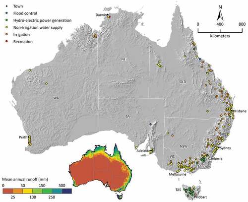
Data defining dam and reservoir features were obtained from two sources: ANCOLD database and the ICOLD database. These two data sets were reduced to include only reservoirs greater than 10 GL in capacity. (Although GL is not an SI unit of measurement, it is a conveniently sized volume for discussing reservoir capacities.) This arbitrary cut-off of 10 GL was based on our Australian experience that smaller reservoirs were constructed mainly for private use, mine water, cooling storages for thermal power stations, small off-stream storages and diversions, industrial cooling water, small recreational lakes, and small-pumped storages. For 224 dams ≥10 GL capacity in the ANCOLD database, 110 climate, hydrology, and terrain attributes were calculated for each dam. More information about the data is provided in the Appendix. In analysis and presentation of the ICOLD data, the Australian dams listed therein are excluded. The locations of the Australian dams are shown in Figure 1.

Figure 1. Locations of the 224 dams and their primary purpose as listed in the ANCOLD database. Inset shows mean annual runoff across Australia.

Although there is a great disparity between the number of dams available for analysis in the two data sets – ANCOLD 224 and ICOLD 10,541 – the sample size of ANCOLD is more than sufficient to allow statistically robust comparisons to be made with the much larger ICOLD sample.

3. Historical development of dam construction in Australia with reference to ANCOLD and ICOLD datasets

The earliest ‘large dam’ constructed in Australia, as recorded in the official record on large dams in Australia, the ANCOLD database, is Lake Parramatta Dam in 1857 (ANCOLD 2010). However, dam building in Australia predates this structure. The earliest dam post-European settlement was a small millpond dam constructed on Norfolk Island in 1795 (Kinstler 2000a) but prior to Europeans settling in Australia, Indigenous Australians are known to have constructed dams for diverting dry season baseflow into adjacent wetlands to enhance food production (Barber and Jackson 2011). However, there is no evidence to date to suggest that any of these structures would have been of large enough to be eligible for inclusion in the ANCOLD database.

The rate of construction of large dams in Australia and the equivalent ICOLD data for developed, developing, and emerging economies are shown in Figure 2(a). This figure shows that generally Australia’s dams were constructed more recently than other developed economies but not as recently as developing and emerging economies. After World War II, the number of dams constructed in Australia increased dramatically as the war had delayed many dam construction projects, electrical authorities were struggling to meet the demand for electricity, and the Federal Government was keen to expand irrigated areas for ‘soldier’ settlers and immigrants (Cole 2000). Analysis of Figure 2(b) shows that prior to 1940 most dams in Australia were constructed in the south-east of the continent, and for the majority, the primary purpose was water supply (Figure 3(a)). Of the dams constructed post-1940, 46% were built in south-eastern Australia and south-west of West Australia, 38% in Queensland and 16% in Tasmania. In Figure 2(a) it is observed that from 1955 to 1980, approximately two-thirds of Australia’s dams and three-fourths of capacity were constructed while a further ~12% were added to the dam stock in terms of numbers and capacity during the following 15 years. Interestingly, however, in terms of total capacity, Australia only started developing dams with large capacities after 1960. Since 1990 the relative increase in the number of dams constructed in Australia (approximately 8%) was similar to the number constructed in other developed economies, but less than those in developing and emerging economies (about 25%).

Figure 2. (a) Cumulative number and cumulative volume of the 224 Australian dams compared with 5023 dams in developing and emerging economies and 4622 dams in developed economics from the ICOLD database. Only dams that were completed after 1850 and have a capacity of 10 GL or greater are included. (b) Spatial distribution of year construction completion of Australian dams.

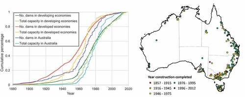
Figure 3. (a) Relationship between latitude and time of completion showing reservoir primary purpose. (b) Relationship between latitude and time of completion showing dam type.

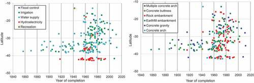
From 1850 to 1950, most dams in Australia (Table 1, Figure 3(b)) and RoW were earth embankments. Their popularity was because they could be constructed on a range of foundation conditions (Watt 2000), whereas gravity dams require sound foundation rock because the leakage path through the foundation under the water barrier is short (Kinstler 2000a).

Post 1950, the availability of large earth moving equipment resulted in larger numbers and higher earth and, in particular, rockfill embankment dams being built in Australia (Cole 2000), while the labour-intensive activities of formwork erection and concrete placing increased the relative costs of concrete dams. Nevertheless, a modest number of concrete gravity dams continued to be built because they could survive overtopping during construction, and concrete dams enabled flood waters to be discharged directly over the dam wall.

From about 1960, rock embankments became a feature in Australian dam building (Table 1). It was found that above a height of 30 m rock embankment dams were more economical than earthfill embankment dams (Cole 2003) because they could be built with much steeper slopes, could be built on a wider range of foundation conditions than arch or gravity dams, could be constructed during rain, and remain stable even under high seepage conditions. Rockfill embankment dams also had the advantage over earthfill embankment dams in that by the 1960s methods had been devised for reinforcing the downstream rockfill slope to protect it from erosion. The high price of mass concrete in Australia after World War II and in the 1970s (Doherty 1999) improved the economics of using rockfill for high dams over concrete structures. Globally, however, earth embankment dams continued to dominate. A possible reason for this follows from the early success of earth embankment dams built in Europe up to the beginning of the nineteenth century (Schnitter 1994). Another possible factor is that overseas dam designers, especially in Europe, were reportedly wary of rockfill structures (Kinstler 2000a) because of some less than satisfactory experiences with concrete face rockfilled dams (e.g. Dix River Dam in Kentucky, USA, and Paradela Dam in Portugal).

Comparatively, the success of early concrete-faced rockfilled dams in Australia, like Cethana in Tasmania, meant their designs were widely adopted (Kinstler 2000a). In fact, of those countries with more than 10 dams >10 GL in the ICOLD database only Norway (65%), Columbia (52%) and Indonesia (41%) have a higher proportion of rock embankment dams than Australia (40%). Interestingly, despite the reportedly large influence of the USA on Australian dam design and construction (e.g. Cole 2000; Eagles 2000; Watt 2000), only 5% of the USA’s dams listed in the ICOLD database are rockfill embankments.

As mentioned earlier, a modest number of concrete gravity dams continued to be constructed in Australia throughout the twentieth century. The exception being in the 1970s when the price of mass concrete became too expensive (Doherty 1999), and there was a lull in construction (Figure 3b). However, in 1984 the first roller-compacted concrete (RCC) dam in Australia, Copperfield River Gorge Dam, was completed in the Gilbert catchment (Forbes and Delaney 1985). This cheaper and quicker method of concrete dam construction (the use of RCC over conventional concrete was estimated to reduce the cost by about 40%, Doherty (1999) has resulted in the proportion of concrete gravity type dams to increase in Australia over the 20-year period between 1990 and 2009 and, since 2010, all large dams constructed in Australia have been RCC dams. Where foundation conditions are suitable RCC dams are generally favoured over embankment dams, particularly in large catchments as it is easier to manage flood events during and after construction. Table 1 presents these observations and we note there that for Australia, rock embankments account for 40% of all dams, concrete gravity accounts for 20%, and 33% are earth embankments. Worldwide, the picture is a little different: rock embankments 13%, concrete gravity dams 17%, and earth embankments 61%.

Table 1 also shows that relatively few concrete buttress dams and arch dams have been constructed in Australia or RoW. Although both types of dams require less concrete than gravity dams they need more formwork and are of greater complexity (Kinstler 2000a). This can be favourable when concrete is expensive and labour is cheap (such as occurred during the Great Depression and after World War II), but in recent decades the high cost of labour has made these types of dams less economical than concrete gravity or embankment dams. Although some arch dams continue to be constructed in the RoW the last large arch and multiple arch dams constructed in Australia were Gordon Dam (1974) and Julius Dam (1976), respectively. Arch dams are generally less suitable in Australia due to a lack of suitable topography; they have greatest benefits over concrete gravity dams where the valley width is narrow and the rock is structurally sound. For example, where the valley width is 400 m arch dams with a cylindrical upstream face require 70% of the concrete compared to that required by a concrete gravity dam, whereas where the valley width is 100 m at the dam crest, arch dams only require 20% of the concrete of a concrete gravity dam (Gehin 1961).

In Table 2, we compare the purpose of reservoirs in Australia with the RoW as recorded in the ANCOLD and ICOLD databases. Water supply is the major purpose (38%) of Australian reservoirs, followed by hydroelectricity at 18% and irrigation at 17%. Of the 224 Australian reservoirs, for which data were available, only one is listed as being used exclusively for flood control and two for recreation. For the RoW, the ICOLD data suggest that irrigation (27%) and hydroelectricity (25%) are the major single purpose reservoirs. Of the Australian reservoirs, 26% were listed as multi-purpose reservoirs, while 29% of global reservoirs were in this category. The main combinations of multi-purpose in Australia were water supply and irrigation (10% of all Australian reservoirs), irrigation and hydroelectric (5%) and water supply and recreation (5%). For the RoW, the main combinations of multi-purpose dams were irrigation and water supply (5% of all RoW reservoirs), all other combinations being less than 3%. Relatively few RoW dams undertake both flood control and supply water for either urban (0.9%) or irrigation (1.0%) use, the dam management objectives for which are conflicting.

Table 3 summarises the site lithology, dam type, and dam height of Australian dams but only dam type and height for the ICOLD data set as no at-site lithology data are available. Additional data for Australian dams are provided in Tables A3 and A4. For the Australian dams, the dam-site lithology favours sediments (60%) over ‘hard rock’ (i.e. igneous and metamorphic rocks) (40%); the median dam height and the inter-quartile range (defined as the difference between the 25^th and 75^th percentiles) of dams located on consolidated and unconsolidated sediments is 41 m (range 21 to 56 m), which is about 3 m more than Australian dams located on hard rock with a median height of 38 m (range 28 to 51 m). For sedimentary sites, two lithologies dominate namely sedimentary siliciclastic rock and regolith. Sedimentary siliciclastic rock underlays 67 dams with a median dam height of 45 m (range 38 m to 67 m). Regolith underlays 41 dams with much smaller dam heights than at other sedimentary sites; the median dam height is 18 m (range 12 to 31 m). The sedimentary quartz-rich arenite to rudite grouping, upon which 10 dams are sited, has the highest median dam wall height (62 m). Igneous felsic intrusive rocks account for 23 dam sites with a median dam height of 51 m (range 39 m to 82 m), and 21 sites are located on igneous felsic-intermediate volcanic with a median height of 44 m (range 37 m to 63 m).

Areas underlain by extensive regolith (e.g. broad valleys) are generally more suited to embankment style dam structures rather than concrete structures which require solid foundation conditions (i.e. fresh bedrock) (Petheram et al. 2013). For this reason, embankment structures tend to be lower in height because of the large cost involved in building wide, high structures. Concrete structures, which have shorter leakage paths, and are required to be constructed on sound foundation bedrock, are most suited to those areas where there is a minimal depth of unconsolidated material (e.g. riverbed sands) that requires excavation (Kinstler 2000a). This tends to occur in more upland areas, which have narrower valleys and greater relief.

4. Australia and the Rest of the World reservoirs compared – simple relationships and patterns

Table 4 provides a summary of the key data of the Australian and the RoW dams that were examined. For each variable, due to the variation in the number of dams with data, all available data were used to calculate the summary statistics

The key observations in Table 4 are:

1. The catchments are in high rainfall and runoff areas (median (mean) values 977 (1002) and 182 (228) mm/year, respectively) relative to the Australian average (mean annual rainfall and runoff of 426 and 43 mm, respectively (BoM 2012; ABS 2008)). Even though Australian dams are in wetter parts of the continent their mean annual runoff is still less than the global mean annual runoff of 280 mm/year (Baumgartner and Reichel 1975).

2. The catchments are mainly forested and have a median slope of 6.9% and a median elevation range of 601 m (definitions are listed in Table A1).

3. The median height of Australian dams is 42 m (the median of the RoW dams is 31 m) and median reservoir capacity is 53 GL (RoW median capacity is 40 GL). The median value of the reservoir capacity/mean annual inflow is 1.29 indicating that more than half the Australian reservoirs are carryover systems (McMahon and Adeloye 2005).

4. The short to moderate height dams (i.e. 75% exceedance and median values) in the Australian dataset are higher than the short to moderate height dams in the RoW dataset. However, high dams (i.e. less than 25% exceedance) in the RoW dataset are higher than high dams in the Australian dataset. We note that the average height of Australian dams has increased by about 0.25 m per year over the last 120 years (plot not shown) compared with RoW increase of 0.34 m per year. These increases are significant because doubling the height of a dam requires a six to eight-fold increase in volume of dam material (Cole 2000).

5. Except for the extremely large reservoirs (less than 0.81% exceedance), the capacities of Australian reservoirs are greater than the RoW reservoirs.

6. Except for the extremely large reservoirs, the surface areas of the Australian and the RoW reservoirs are similar.

7. The median value of specific spillway capacity of Australian dams is 3.9 m³/s/km² (mean 6.2) and RoW is 1.9 m³/s/km² (mean 7.2).

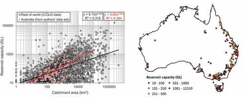
In the next three figures, we explore the correlations among reservoir capacity, reservoir surface area at FSL and catchment area for Australia and the RoW. Figure 4(a) is a plot of reservoir capacity and catchment area and is particularly interesting because at a catchment area of approximately 323 km² (the median area of 176 Australian catchments in Table 4) the reservoir capacity in Australia is 1.3 times that for the RoW. At 1000 km² the ratio is 1.6. This increased size provides empirical evidence for the previous hypothetical storage-yield analysis (where reservoir evaporation was neglected) (McMahon et al. 2007), which concluded that the reservoir capacities required in Australia are, relatively speaking, larger than those observed in the RoW. This is attributed to Australian rivers exhibiting the largest inter-annual variability in streamflow for temperate (Peel, McMahon, and Finlayson 2004) and tropical (Petheram, McMahon, and Peel 2008) regions of the world. In Figure 4(b) most of the reservoirs with a capacity greater than 1000 GL are found in south-eastern Australia and Tasmania. Only three are in northern Australia – Fairbairn, Burdekin, and Ord River dams.

Figure 4. (a) Relationship between reservoir capacity and catchment area comparing 176 Australian reservoirs with 3819 from the rest of world. (b) Spatial distribution of reservoir capacity of Australian reservoirs. Note the Australian reservoirs are on-stream storages and do not include run-of-river systems associated with hydroelectricity generation, weirs, barrages, and diversions.

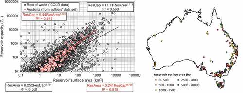
Figure 5(a) is a plot of reservoir capacity and reservoir surface area in which 220 Australian reservoirs are compared with 6990 reservoirs from the RoW. The Australian data exhibit a high correlation and provide a guide to estimate the reservoir capacity of an existing dam based on reservoir surface area. This strong relationship, which accounts for 81% of the variance in the dependent variable, is potentially useful because often surface area can be derived from satellite imagery, but reservoir capacity cannot be estimated that way. Conversely, the inverse relationship may be helpful in parameterising existing dams in continental and global models where information on capacity has been recorded but the surface area is unavailable (32% of reservoirs in the ICOLD database with capacity ≥10 GL do not have surface area data). Figure 5(b) shows the spatial distribution of reservoir surface area across Australia.

Figure 5. (a) Relationship between reservoir capacity and reservoir surface area (≥0.1 km²) comparing 220 Australian reservoirs with 6990 from the rest of world. The equations for the least squares inverse relationships are shown below the figure. (b) Spatial distribution of reservoir surface area of Australian reservoirs.

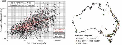
Figure 6(a) is a plot of reservoir surface area and catchment area comparing 214 Australian reservoirs with 3548 from the RoW. The lines of best fit to both data sets, which account for a low proportion of the variance, do have different slopes and diverges by about half log cycle for small catchment areas although there is little difference between the two data sets. The spatial distribution of the catchment areas for each of the Australian reservoirs is shown in Figure 6(b).

Figure 6. (a) Relationship between reservoir surface area (≥0.1 km²) and catchment area comparing 214 Australian reservoirs with 3548 from the rest of world. (b) Spatial distribution of catchment area of Australian reservoirs.

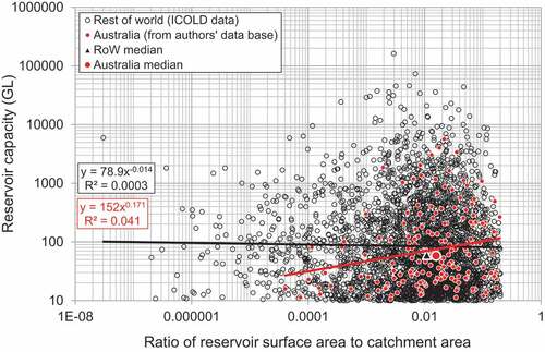
Two other relationships were explored – dam height and reservoir capacity, and reservoir capacity and the ratio of reservoir surface area to the catchment area. These yielded very weak relationships and the plots are presented as Figures A1 and A2.

In Figure 7, reservoir capacity divided by reservoir surface area is plotted against dam wall height in which the Australian and the global relationships account for 82% and 68% of the variance, respectively. The regression coefficients of the two datasets are both 0.27, pointing to a universal relationship. Excluding evaporation, data points above the regression line are reservoirs that are more efficient in storing water than those below the line. This suggests the dimensionless metric, ResVol/ResArea/DamHt, is a site efficiency metric with respect to storing water. For Australia, the median value is 0.27 with an inter-quartile range of 0.22 to 0.32 and for the RoW, the median value is 0.29 with a range of 0.22 to 0.38. The slightly lower Australian values compared to the RoW indicate that Australian reservoirs are a little less efficient than RoW or that Australian dams have a larger allowance for flood surcharge above the FSL, or a combination of both.

Figure 7. (a) Relationship between reservoir capacity divided by reservoir surface area and dam height comparing 102 Australian reservoirs with 6374 from the rest of world. (b) Spatial distribution of reservoir capacity divided by reservoir surface area and by calculated trend line value in Figure 7a of Australian reservoirs.

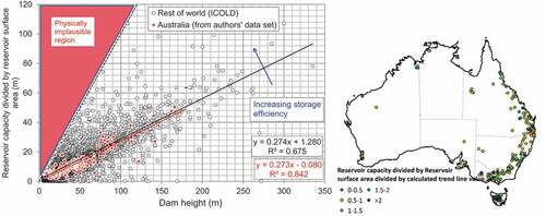
Correlation analysis using the Australian data suggests the DimVol metric is virtually unrelated to the dam location or to catchment attributes related to topography, the largest correlation between DimVol and the attributes is −0.21 which relates to elevation range. Figure 7(b) shows the spatial distribution of DimVol and that reservoirs in south-eastern Australia and Tasmania generally have higher storage efficiencies than reservoirs in Queensland and other parts of northern Australia.

For 1500 randomly selected potential dam sites across a wide variety of landscapes in the northern half of Australia (for which datasets were readily available from Petheram et al. (2014) and were not influenced by anthropogenic change), it was found that the reservoir volume divided by reservoir surface area was equal to the full supply level height multiplied by 0.30 + 1.31. This is slightly higher than the RoW and Australian relationships shown in Figure 7(a) and could be explained by the fact that the heights listed in the ANCOLD and ICOLD databases are the heights of the dam wall crests (i.e. dam abutments) not the FSL (i.e. the spillway). Conceptually, the difference between this ‘northern Australian’ relationship at the FSL and the RoW and Australian relationships for the dam wall crest, shown in Figure 7(a), is due to the allowance of flood surcharge (i.e. the difference between the maximum dam and saddle dam height and the FSL) in the latter relationships (i.e. RoW and Australian relationships).

To explore the potential relationships based on Australian data between dam height and dam length and at-site, catchment, climate and hydrologic attributes, regression analyses were performed. Details are provided in Appendix and, in the main with the exception of the spillway capacity relationships, the relationships (Table A5) are not particularly strong.

5. Australia and rest of world spillways compared – simple relationships and patterns

For the 211 Australian spillways for which data are available, 24% are controlled by gates and the remainder are uncontrolled. For the 4570 RoW spillways, the proportion of controlled and uncontrolled spillways is 45% and 55%, respectively. The lower proportion of gated spillways in Australia may be because reportedly some dam authorities in Australia have been reluctant to instal gates in case they fail to open or inadvertently open and cause flooding downstream (Kinstler 2000b). Although limited data are available for Australia, a considerable number of RoW dam failures has been attributed to the malfunction and operational mismanagement of gates under flood conditions (ANCOLD 1994). In the following paragraphs, some simple relationships are explored.

Figure 8. (a) Relationship between spillway capacity and catchment area comparing 184 Australian reservoirs with 1706 from the rest of world. (b) Spatial distribution of spillway capacity of Australian reservoirs.

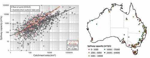
Figure 9. (a) Relationship between specific spillway capacity and catchment area comparing 184 Australian reservoirs with 1706 from the rest of world and with envelope of largest global discharges. (b) Spatial distribution of specific spillway capacity of Australian reservoirs.

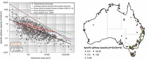
In Figure 8(a) spillway capacity is related to the catchment area. For Australia, 54% of the variance is accounted for in logarithmic space and 46% for the RoW. The line of best fit for the Australian data is above the RoW line and at the median catchment area of 323 km² the ratio between the average Australian spillway capacity and RoW value is 1.9. Given the influence of climate on flood design hydrology, it is surprising that no spatial pattern of spillway capacity or specific spillway capacity is evident in Figure 8(b) or 9(b). When spillway capacity per unit area is related to the catchment area, the strength of the relationship weakens for Australia yet increases for the RoW (Figure 9(a)). However, in Figure 9(a) the two variables cannot be considered to be independent because both are a function of area and, consequently, the statistics of the relationships are spurious (Kenny 1982). Nevertheless, the plot is interesting as it can be related to a threshold of maximum observed discharges. In Figure 9(a) the plotted threshold equation by Francou & Rodier (1967) as detailed by Rodier and Roche (1984) is given by Equation 1(1) $q=\frac{1}{A}\left({10}^{\left(\left(\frac{\left(10-K\right)}{10}\left(log10\left(A\right)-8\right)\right)+6\right)}\right)$(1) and the plotted threshold equation by Nathan, Weinmann, and Gato (1994) is given by Equation 2(2) $q=\frac{129.1A^{0.616}}{A}$(2) :

(1) $q=\frac{1}{A}\left({10}^{\left(\left(\frac{\left(10-K\right)}{10}\left(log10\left(A\right)-8\right)\right)+6\right)}\right)$(1)

(2) $q=\frac{129.1A^{0.616}}{A}$(2)

where $q$ is the threshold of recorded maximum discharge (m³/s/km²), $A$ is catchment area (km²) and $K$ is a coefficient. For catchments >100 km²; we adopted $K$ = 6 in Figure 9(a) as recommended by Rodier and Roche (1984, 343). It is observed in Figure 9(a) that the maximum capacities of Australian and the RoW spillway are similar to those based on the threshold curve of Francou and Rodier (1967). The third envelope in Figure 9(a), which is an empirical equation and captures nearly all but one extreme value, is:

(3) $q=6000A^{-0.8}$(3)

where the symbols are defined earlier. Based on Figure 9(a) we note that, in the range of catchment areas 100 to 10,000 km², Australian spillway capacities per catchment area are among the largest worldwide. This observation is consistent with earlier analysis that shows specific flood discharges of 1% annual exceedance probability (AEP) for Australia are larger than 1% AEP values for ROW (McMahon et al. 1992) and that the threshold curve of Nathan, Weinmann, and Gato (1994) based on Australian PMF studies exceeds that of Francou and Rodier (1967) for catchment areas greater than 1000 km². However, this observation is also likely because in many parts of the RoW (e.g. Europe) dams are often designed for a 1 in 10,000 AEP, whereas in Australia many dams are designed for the probable maximum flood, particularly where dam failure would result in loss of life (ANCOLD 2000). It should be noted that many parts of RoW use a ‘standards based’ approach to flood estimation, whereas Australia has moved to a ‘risk based’ approach, and due to differences in the design philosophy of the two approaches, the AEP is not directly comparable (Nathan and Weinmann 2004). The RoW data in Figure 9(a) show that the constructed spillway capacities in the Australian dataset and RoW dataset vary over two and three orders of magnitude, respectively, leading one to question whether some of the reservoirs with the lower capacities have adequate spillway protection. Inadequate spillway capacity has been identified as a major cause of dam failure around the world (ANCOLD 2000). In Figure 9(b) specific spillway capacities are generally largest near major population centres (e.g. Melbourne, Sydney, Brisbane, Perth, and Adelaide). This is likely to be due to dams in these areas being designed to safely discharge floods of higher AEP (i.e. most likely the probable maximum flood) than dams in more remote settings.

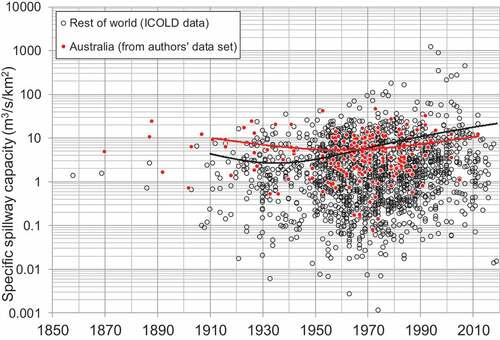
There is little evidence of an increase in specific spillway capacity in the Australian dataset (Figure 10) because Australian dams have systematically had their spillways upgraded over time. The RoW dataset showed stronger evidence of an increase in specific spillway capacity over time from an average of 5 to 19 m³/s/km² (Figure 10) indicating that there may be many older dams in the RoW for which the spillway capacity has not been increased with changes to flood design estimation methods and more stringent dam safety measures. Alternatively, spillway upgrades may not have been recorded in the ICOLD database.

Figure 10. Specific spillway capacity versus year of completion of dam construction for 184 Australian and 1617 RoW dams. The curves of best fit exclude data prior to 1910.

6. Regression analyses associated with dam height, dam length and spillway capacity and at-site, catchment, and climate attributes for Australian dams and reservoirs

To explore the potential relationships based on Australian data between dam height, dam length on one hand, and spillway capacity and at-site, catchment, climate, and hydrologic attributes on the other, regression analyses were performed.

6.1. Method

For each dependent variable (dam height, dam length, and spillway capacity) an initial preliminary step-wise regression was carried out. The analyses proceeded as follows:

1. A preliminary step-wise regression was applied using 110 cardinal variables (one dependent variables plus 109 ‘independent’ variables), and the so-called independent variables that were identified by this regression were screened for the variance inflation factor (VIF) which identifies collinearity or cross-correlation in the independent variables. Independent variables with the largest VIFs were progressively eliminated by ordinary least squares (OLS) regression with the objective of finally accepting only independent variables with a VIF value ≤3 and the median of all the VIF values ≤2. Some researchers have applied a less restrictive rule (see O’Brien 2007 for comments) but in adopting the above criterion we were cognisant of O’Brien’s advice that ‘…. threshold values of the VIF (and tolerance) need to be evaluated in the context of several other factors that influence the variance of regression coefficients’. We followed this advice by checking that the cross-correlation matrices of the independent variables incorporated in the adopted regression model were low.

2. Adopting the independent variables found under item 1, the dependent variables were then subjected to a Box-Cox analysis with λ varying from 0 (ln transformation) through 0.5 (square root transformation) and, finally, to 1 (no transformation). Separately, a log₁₀ transform was applied to all the variables and a step-wise regression performed. Further OLS regressions were carried out as appropriate.

3. The Anderson-Darling (A-D) statistic was adopted to ensure the residuals were normally distributed using the 95% confidence level. For this case, the p-statistic needs to be >0.05 (Anderson and Darling 1952). In a few cases where the plots of residuals appear to be normally distributed but were rejected by the A-D test due to several outliers, these were deleted and the A-D test applied again.

4. The p-values of regression coefficients were also scrutinised to ensure the regression coefficients were different from zero at the 0.05 level of significance and the signs of the regression coefficients were consistent with the physical processes.

Following the above steps, regression equations were developed for the following three dependent variables – dam height, dam length, and spillway capacity – yielding four equations for each variable (one for all dam types combined, and three based on earthfill embankments, rockfill embankments, and concrete gravity embankments). Equations for spillway capacity are listed in Table 5. Equations for dam height and length, although interesting, have little application in a pre-feasibility analysis and, consequently, are listed in Table A5. For each equation, we report the sample size (N), R²(adj) (which indicates how much the predictors explain the dependent variable taking into account the number of predictors), R²(pred) (which indicates the predictive ability of the model), S (which is the square root of the mean square error in the units of the dependent variable), along with comments. Under comments the following information is included: the type of regression model, VIF range and median values, A-D test for normality, and regression coefficient (Reg. coeff.) (which indicates whether the regression coefficients are statistically significant from zero). In the equations in Table 5, ‘L’ at the beginning of all variables in an equation indicates the regression analysis was carried out in log₁₀ space. Where there were zero or negative values for an independent variable, a slightly smaller value than the minimum value in the series was added to all values to ensure that a logarithmic transformation is possible.

6.2. Results

Based on a review of the equations in Table 5 and Table A5, we summarise in Table 6 the key independent variables driving the relationship for all dam types, combined or individually. The following comments relate to all dam types combined. With regard to dam height, reservoir capacity (ResVol) accounts for 30% of the variance and 56% if the standard deviation of valley bottom flatness (MrVBFSD) is linearly combined in log space with ResVol. For dam wall length, the mean valley bottom flatness explains 39% of the variance, and for spillway capacity, catchment area is the key variable and accounts for 62% of the variance. In the case of dam height, adding a second variable nearly doubles the variance accounted for; for dam length and spillway capacity, a second variable made little difference to the magnitude of the variance accounted.

Table 6. Key independent variables that contribute to dam height, dam wall length and spillway capacity.

Dam types	Dependent variable	Independent variable 1	Variance	Adding independent variable 2	Variance of 1 + 2
Dam height
All dam types	LDamHt^a	LResVol	30%	LMrVBFSD	56%
Earthfill embankment	DamHt	MrVBFFocMea	37%	ResVol	60%
Rockfill embankment	(DamHt)^0.5	ElRa	37%	MrVBFF0cMea	47%
Concrete gravity	DamHt	ResVol	37%	RuAnnMea	55%
Dam length
All dam types	DamLeng	MrVBFBufMea	39%	No variable	-
Earthfill embankment	DamLeng	MrVBFBufMea	28%	No variable	-
Rockfill embankment	DamLeng	MrVBFBufMea	41%	RunAnnMea	52%
Concrete gravity	DamLeng	MrVBFBufMea	29%	SandRa	47%
Spillway capacity
All dam types	(LSpillCap)^1.541	LCatchArea	62%	LResArea	67%
Earthfill embankment	LSpillCap	LCatchArea	58%	No variable	-
Rockfill embankment	LSpillCap	LCatchArea	58%	LResArea	70%
Concrete gravity	LSpillCap	LRuAnnSD	55%	LDamHt	65%

^aDefinitions of variable names are given in Table 5 and as follows. DamLeng, Length of dam wall; ResVoL, Reservoir volume; MrVBFFocMea, Mean of 1 km buffer dam wall focal range; MrVBFSD, Standard deviation of MrVBF; ElRa, Range of elevation; SandRa, Range of sand; RuAnnMea, Mean annual runoff; RuAnnSD, Standard deviation of annual runoff.

7. Discussion

An empirical analysis of the ANCOLD dataset largely confirms existing narratives on Australian dam construction. However, one observation that was difficult to resolve was a statement made by numerous and qualified authors that Australian dam design and construction were strongly influenced by practices in the USA, yet Australia has an unusually high proportion of rockfilled dams (40%) whereas in the USA only 5% of dams are recorded as being rockfilled.

The physical characteristics of Australian dams differ to the RoW dam dataset in various ways. For a given catchment area Australian dams were found to have relatively larger reservoir capacities and larger spillway capacities than dams from the RoW. This observation is consistent with a previous hypothetical storage-yield analysis comparing Australian dams to those from the RoW. For a given reservoir capacity, the height of dam walls in Australia is generally higher than dams of equivalent capacity from the RoW. However, the surface areas of Australian and RoW reservoirs tend to be similar at equivalent reservoir capacities.

Excluding evaporation, a comparison of the databases indicates that Australian dams are less efficient in storing water than dams from RoW. Given that the annual inflows into dams from the RoW are likely to be larger than the inflows to dams in Australia (as a result of larger catchment areas and higher mean annual runoff per unit area), this would suggest that Australian dams result in a higher degree of regulation (e.g. the ratio of controlled flow and net evaporation to uncontrolled releases) than dams from the RoW. This is consistent with the observation by McMahon et al. (1992) that Australian rivers require relatively larger reservoirs for a given draft and reliability of supply than RoW rivers.

8. Conclusion

This paper is centred on the premise that understanding the history, the characteristics of Australian dams and related infrastructure and their global setting better inform water resources engineering decision-making. Large infrastructure projects are often initiated through a pre-feasibility study. This is especially so for water engineering projects involving dams. Currently, there is a move towards water resources development in northern Australia, including interest in large dams and irrigation. Globally, hydropower is a major driving element. A pre-feasibility study involving dam construction requires, among other things, an understanding of the site conditions, the catchment hydrology, an estimate of the reservoir volume, dam size and type, and spillway capacity. This paper, which addresses these latter aspects, together with our complimentary paper dealing with dam costs provides information required to inform a pre-feasibility study. Understanding the historical setting of an infrastructure element, e.g. a dam or spillway or how the size compare with global values, provides decision-makers with greater confidence in the pilot values adopted. This paper addresses both the history and global setting dams, reservoirs, and spillways. We offer the following conclusions which are based on reviewing the history of dam building in Australia and on analysis of data for 224 Australian reservoirs and for approximately 10,500 reservoirs in the Rest of the World (RoW), all greater than 10 GL in capacity.

1. Most Australian dams are located within a 200-km band along the eastern and southern (Victorian) coastlines of Australia.

2. 90% of capacity of Australian reservoirs were constructed over the 40-year period beginning in 1960. This is based on two-third of the dams constructed since the first in 1857.

3. Forty per cent of Australian dams are rock embankments (RoW 13%), concrete gravity accounts for 20% (RoW 17%), and 33% are earth embankments (RoW 61%).

4. Water supply is the major purpose (38%) of Australian reservoirs, followed by hydroelectricity at 18% and irrigation at 17%. For the RoW, irrigation (27%), and hydroelectricity (25%) are the major single purpose reservoirs. Twenty-six per cent and 29% of Australian and RoW reservoirs, respectively, are multi-purpose.

5. For Australian dams, the dam-site lithology favours sediments (60%) over hard rock (40%) with a small median height difference of 41 m (sediments) compared with 38 m, respectively (hard rock).

6. The median values of the ratio, reservoir capacity/mean annual inflow, is 1.29 indicating that more than half the Australian reservoirs are carryover systems.

7. Except for the extremely large reservoirs, the capacities of Australian reservoirs are greater than the RoW reservoirs although the reservoir surface areas are similar.

8. Australian reservoirs with catchment areas of 323 km² and 1000 km² have a capacity 1.3 and 1.6 times, respectively, that of reservoir capacities for the RoW. This increased size provides empirical evidence for previous hypothetical storage-yield analysis (where reservoir evaporation was neglected) (McMahon et al. 2007), which concluded that the reservoir capacities required in Australia are, relatively speaking, larger than those observed in the RoW.

9. A measure of site efficiency with respect to storage is the regression coefficient of a plot of reservoir capacity divided by reservoir surface area against dam wall height. For both ANCOLD and ICOLD data sets, the regression coefficient is 0.27. The efficiency of storage of individual reservoirs can be compared with this value, larger values are more efficient.

10. One-quarter of Australian spillways are controlled by gates; the remainder are uncontrolled. For RoW spillways, the proportion of controlled and uncontrolled spillways is 45% and 55%, respectively.

11. Spillway capacity is related to the catchment area, but the relationship is not strong; for Australia and RoW, about 50% of the variance is accounted. Our analysis suggests for the median Australian catchment area the ratio between the average Australian spillway capacity and RoW value is 1.9.

12. Because Australian dams have had their spillways upgraded over time and these upgrades have been recorded in the ANCOLD database, there is little evidence of an increase in specific spillway capacity. This contrasts with the RoW dataset where there is stronger evidence of an increase in specific spillway capacity over time, indicating that there may be many older dams in the RoW for which the spillway capacity has not been increased with changes to flood design estimation methods and more stringent dam safety measures. Alternatively, spillway upgrades may not have been recorded in the ICOLD database.

Acknowledgments

We are especially grateful to Graeme Bell and Rory Nathan who straightened us out on several key issues. We would like to acknowledge ANCOLD and ICOLD for their efforts in maintaining registers of large dams in Australia and globally, respectively. We are grateful to two anonymous reviewers, who provided helpful advice in an earlier manuscript, and to the Editor and two other reviewers for their comments regarding the manuscript which formed the basis of this paper.

Additional information

Funding

No funding was received for this work.

Notes on contributors

T. A. McMahon

T. A. McMahon has contributed extensively to understanding Australia’s surface hydrology and water resources. During his career he has published 7 books and manuals and more than 550 book chapters, scientific papers, reports and articles on hydrology and water resources engineering. One of his many career highlights was introduction of reservoir storage-yield-reliability procedures to the Australian water engineering profession in the early 1970s. In recent years he has been involved in research into large-scale atmospheric drivers for hydrologic variability, the estimation of evaporation from standard meteorological data, and uncertainty in future streamflow estimates based on climate models.

C. Petheram

C. Petheram is a hydrologist and principal research scientist at CSIRO, Australia. He has a BEng from the University of Melbourne and a PhD inhydrology with the CRC for Catchment Hydrology and University of Melbourne. Since joining CSIRO in 2004 Cuan has worked on many large water and agricultural resource assessment projects across northern Australia. Most recently he was the lead author on the Northern Rivers and Dams report (2014), an appendix to the Northern Australia White Paper (PMC 2015) and he was the joint project manager of the Northern Australia Water Resource Assessment (2016–2018) and the Flinders and Gilbert Agriculture Resource Assessment (2012–13).

Appendix

Table A1 summarises the number and types of variables available for detailed analyses of the Australian data in which dam height and dam length are related to at-site, catchment, climate, and hydrology attributes. These attributes or variables are detailed in Tables A2–A4. Of the 133 attributes, 112 are primary cardinal attributes, 13 are secondary cardinal attributes and 8 are nominal attributes. Dam and reservoir details were obtained from the ANCOLD database. Where erroneous values were identified they were either corrected, if authoritative information were available (i.e. a published study) or removed from the analysis.

To calculate location details, terrain, climate, and hydrological attributes, each dam was manually geo-referenced using an iterative process by locating the dam and reservoir on Google Earth and then positioning a point representation of the dam on a flow accumulation grid of the third version of the 9 second DEM (Hutchinson et al. 2008). Attributes were either calculated ‘at-site’ or for the dam’s contributing area or catchment. At-site calculations involved either assigning an attribute value based on the point location of the dam or calculating an average attribute value within a specified radius of each dam site. In some instances, at-site attribute calculations were confounded by missing data due to the presence of the reservoir. For example, for those reservoirs that were in existence prior to the development of the 9 second DEM, terrain attribute datasets returned null values over that portion of the dataset that intersected the reservoir. In these instances, and where average attributes were being calculated within a specified radius of a dam, the null values were ignored.

The upstream contributing area to each dam was derived using the third version of the 9 second DEM. The resulting catchment boundaries were used to determine catchment attribute information and to calculate inflows from gridded runoff surfaces. Climate data (1930 to 2007) were obtained from the SILO 0.05 degree gridded climate dataset of Australia (Jeffrey et al. 2001). Gridded daily runoff surfaces (1930 to 2007) at 0.05 degree resolution covering Australia were obtained from data sets developed by Petheram et al. (2012) and Vaze et al. (2013).

Of the 565 entries in the ANCOLD database, 237 reservoirs have reservoir capacities ≥10 GL. Thirteen entries were removed because they were saddle dam structures or could not be geographically located, leaving 224 reservoirs ≥10 GL in capacity available for further analysis. Of the 224 large reservoirs, some were missing at-site or catchment data or data for dam features, for example dam length or volume, leaving 217 dams with most data items. However, of these, 41 are off-stream storages, have negligible-sized catchments, are run-of-river storages associated with hydropower generation, or are weirs and diversions, leaving 176 on-stream storages with a storage capacity ≥10 GL.

Analysis of dam heights

Dam heights versus reservoir capacities comparing Australia and RoW are plotted in Figure A1(a). For a reservoir of capacity 53 GL (the median capacity of the Australian data set), the height of an Australian dam is 36.1 m compared with the RoW value of 30.0 m. The highest dams are situated in south-eastern Australia and Tasmania. With one exception all dams in Queensland and northern Australia are less than 75 m in height (Figure A1(b)).

Although the data in Figure A1(a) show considerable variation, at a given site a useful relationship between reservoir capacity and water level height emerges. Because the height–reservoir area–reservoir capacity relationships were not available for the majority of dams in the ANCOLD or ICOLD database, 1500 potential dam sites across a wide variety of landscapes in the northern half of Australia (for which datasets were readily available from Petheram et al. (2014), and over which there is negligible anthropogenic influences on the DEM, e.g. existing reservoirs) were randomly selected and height-reservoir area-reservoir capacity relationships derived for each. It was found that for a given site halving the reservoir capacity occurs, on average, 0.794 times the original height. This empirically derived result perfectly matches the theoretical result, where if a reservoir is assumed to have a triangular surface where both length (bh) and dam width (ah) increase linearly with water height (h), the volume (V) is the integral of area (Equation A1)(A1) $A=\frac{ab{h}^2}{2}$(A1) over height (Equation A2)(A2) $V=\frac{ab{h}^3}{6}$(A2) . This cubic dependency means that for a given site half the reservoir capacity will occur at 0.794 of the height. This information can be usefully applied to derive a height–volume relationship for reservoirs where only the FSL height and capacity are known.

(A1) $A=\frac{ab{h}^2}{2}$(A1)

(A2) $V=\frac{ab{h}^3}{6}$(A2)

A measure of spatial significance is plotted in Figure A2 where the reservoir capacity is correlated with the ratio of reservoir surface area to the catchment area. Based on these data, 75% of Australian reservoirs have a ratio >0.006 whereas for the global reservoirs the ratio for 75% exceedance is 0.003. In the analysis, the ratio was restricted to less than 0.2, ensuring that most off-stream and run-of-river storages were not included in the plot. For the Australian data (n = 184) the median capacity is 58 GL and the median ratio of areas is 0.016, in other words, for the median reservoir capacity the catchment area is typically 60 times larger than the reservoir area at FSL. The equivalent values for the RoW (n = 3505) are for the median reservoir capacity of 60 GL the catchment area is 90 times larger than the reservoir area at FSL.

Regression analysis relating dam height, dam length and spillway capacity to at-site, catchment, and climate attributes

To explore the potential relationships based on Australian data between dam height and dam length and at-site, catchment, climate, and hydrologic attributes, regression analyses were performed as follows:

1. A preliminary step-wise regression was applied using 110 cardinal variables (one dependent variable plus 109 ‘independent’ variables), and the so-called independent variables that were identified by this regression were screened for the variance inflation factor (VIF) which identifies collinearity or cross-correlation in the independent variables. Independent variables with the largest VIFs were progressively eliminated by ordinary least squares (OLS) regression with the objective of finally accepting only independent variables with a VIF value ≤3 and the median of all the VIF values ≤2. Some researchers have applied a less restrictive rule (see O’Brien, 2007 for comments) but in adopting the above criterion we were cognisant of O’Brien’s advice that ‘…. threshold values of the VIF (and tolerance) need to be evaluated in the context of several other factors that influence the variance of regression coefficients’. We followed this advice by checking that the cross-correlation matrices of the independent variables incorporated in the adopted regression model were low.

2. Adopting the independent variables found under item 1, the dependent variables were then subjected to a Box-Cox analysis with λ varying from 0 (ln transformation) through 0.5 (square root transformation) and, finally, to 1 (no transformation). Separately, a log₁₀ transform was applied to all the variables and a step-wise regression performed. Further OLS regressions were carried out as appropriate.

3. The Anderson-Darling (A-D) statistic was adopted to ensure the residuals were normally distributed using the 95% confidence level. For this case, the p-statistic needs to be >0.05 (Anderson and Darling, 1952). In a few cases where the plot of residuals appears to be normally distributed but was rejected by the A-D test due to several outliers, these were deleted and the A-D test applied again.

4. The p-value of regression coefficients was also scrutinised to ensure the regression coefficients were different from zero at the 0.05 level of significance and the signs of the regression coefficients were consistent with the physical processes.

Following the above steps, regression equations were developed for two dependent variables – dam height and dam length – yielding four equations for each variable (one for all dam types combined, and three based on earthfill embankments, rockfill embankments and concrete gravity embankments) and results are presented in Table A5. For each equation, we report the sample size (N), R²(adj) (which indicates how much the predictors explain the dependent variable taking into account the number of predictors), R²(pred) (which indicates the predictive ability of the model), S (which is the square root of the mean square error in the units of the dependent variable), along with comments. Under comments the following information is included: the type of regression model, VIF range and median values, A-D test for normality, and regression coefficient (Reg. coeff.) (which indicates whether the regression coefficients are statistically significant from zero). In the equations in the table, ‘L’ at the beginning of all variables in an equation indicates the regression analysis was carried out in log₁₀ space. Where there were zero or negative values for an independent variable, a slightly smaller value than the minimum value in the series was added to all values to ensure that a logarithmic transformation is possible.

References relevant to Appendix

Anderson TW, Darling DA. 1952. “Asymptotic Theory of Certain ‘Goodness-of-Fit’ Criteria Based on Stochastic Processes.” Annals of Mathematical Statistics 23: 193–212.

Gallant J, Austin J. 2012. Prescott Index derived from 1 “ SRTM DEM-S. v2. CSIRO. Data Collection. https://doi.org/10.4225/08/53EB2D0EAE377

Hutchinson MF, Stein JL, Stein JA, Anderson H, Tickle PK. 2008. “GEODATA 90 second DEM and D8: Digital Elevation Model Version 3 and Flow Direction Grid 2008”. Metadata file identifier: a05f7892-d78 f-7506-e044-00144fdd4fa6. Accessed March 2011. http://www.ga.gov.au/metadata-gateway/metadata/record/gcat_66006

Jeffrey SJ, Carter JO, Moodie KM, Beswick AR. 2001. “Using spatial interpolation to construct a comprehensive archive of Australian climate data.” Environmental Modelling & Software 16(4): 309–330.

O’Brien RM. 2007. “A caution regarding rules of thumb for Variance Inflation Factors” Quality & Quantity 41: 673–690.

Petheram C, Rustomji P, McVicar TR, Cai W, Chiew FHS, Vleeshouwer J, Van Niel TG, Li L, Cresswell RG, Donohue RJ, Teng J, Perraud J-M. 2012. “Estimating the Impact of Projected Climate Change on Runoff Across the Tropical Savannas and Semiarid Rangelands of Northern Australia”. Journal of Hydrometeorology 13: 483–503. doi: 10.1175/JHM-D-11-062.1.

Vaze J, Viney N, Stenson M, Renzullo L, Van Dijk A, Dutta D, Crosbie R, Lerat J, Penton D, Vleeshouwer J, Peeters L, Teng J, Kim S, Hughes J, Dawes W, Zhang Y, Leighton B, Perraud J.M, Joehnk K, Yang A, Wang B, Frost A, Elmahd A, Smith A. and Daamen C. 2013. “The Australian Water Resource Assessment System (AWRA).” Proceedings, 20th International Congress on Modelling and Simulation (MODSIM2013). Australia: Adelaide.

Table A1. List of symbols.

Variable	Symbol	Variable	Symbol
Elevation
The elevation range measures the full range of elevations within a circular window and can be used as a representation of local relief. Elevations are approximate AHD.
Mean elevation (m)	ElMea	Minimum elevation (m)	ElMin
Standard deviation of elevation (m)	ElSD	Maximum elevation (m)	ELMax
Range of elevation (m)	ElRa
Woody Non-woody
A woody/non-woody raster: 1 signifies woody, 0 signifies non-woody. Value is a catchment average.
Mean woody1, non-woody0	Woody
Slope
Slope measures the inclination of the land surface from the horizontal. Percent slope represents this inclination as the ratio of change in height to distance. The focal median of percent slope can be used as a surrogate for modal slope in landform pattern analysis.
Mean slope (%)	SlMea	Standard deviation of slope (%)	SlSD
Profile curvature
Profile curvature is the rate of change of potential gradient down a flow line and represents the changes in flow velocity down a slope. It is significant for flow acceleration, erosion/deposition rates and geomorphology.
Mean profile curvature (radian/m)	ProCurvMea
Plan curvature
Plan (or contour) curvature is the rate of change of aspect (orthogonal to the slope) and represents topographic convergence or divergence. It is significant for water movement across the landscape, i.e. the accumulation or dispersion of water.
Mean plan curvature (radian/m)	PlanCurvMea
Clay/Sand
Mean clay (%)	ClayMea	Mean sand (%)	SandMea
Standard deviation of clay (%)	ClaySD	Standard deviation of sand (%)	SandSD
Range of clay (%)	ClayRa	Range of sand (%)	SandRa
Multi-resolution valley bottom flatness
Multi-resolution Valley Bottom Flatness (MrVBF) is a topographic index designed to identify areas of deposited material at a range of scales based on the observations that valley bottoms are low and flat relative to their surroundings and that large valley bottoms are flatter than smaller ones. Units are dimensionless.
Mean MrVBF	MrVBFMea	Range of MrVBF	MrVBFRa
Standard deviation of MrVBF	MrVBFSD
Multi-resolution valley bottom flatness 1 km buffer dam wall
This is the average MrVBF value within a 1 km radius of the centroid of the dam wall. Units are dimensionless.
Mean 1 km buffer dam wall MrVBF	MrVBFBufMea	Mean 1 km buffer dam wall focal range	MrVBFFocMea
Standard deviation of 1 km buffer dam wall MrVBF	MrVBFBufSD	Standard deviation of 1 km buffer dam wall focal range	MrVBFFocSD
Koppen
Estimated at dam wall. See Table S2 for definitions.
Köppen-Geiger class	Koppen
Lithology
Estimated at dam wall using Surface Geology of Australia 1:1 million scale dataset 2012 edition. Description of rock types are given in the text. See Table A3
Dam wall Lithgroup	DamLith
Location
Dam wall latitude (degree)	Lat	Dam wall longitude (degree)	Long
Other
Year of completion	YrComp	State of Australia in which dam is located	State
Years to construct	YrsConstr	Distance from closest capital city	Dist
Dam characteristics
We use the terms ‘dam wall’ and ‘spillway’ for each entity and the term ‘dam’ to mean the wall and spillway; the term ‘reservoir’ is the body of water held upstream by the wall.
Dam type	DamType	Volume of wall (10^3 m^3)	DamVol
Dam face	DamFace	Spillway capacity (m^3/s)	SpillCap
Height of dam (m)	DamHt	Spillway capacity per catchment area (m^3/s/km^2)	SpillCap/Area
Length of wall (m)	DamLeng	Freeboard (m)	FBoard
Dam foundation	DamFdn
Reservoir characteristics
Reservoir volume (10^3 m^3) Estimated at full supply level. In some plots we use ML (= 10^3 m^3) or GL (= 10^3 m^6)	ResVol	Reservoir volume/mean annual flow (year^−1)	ResVol/MAR
Reservoir volume (GL)	ResVolGL	Reservoir volume/reservoir surface area (m)	ResVol/Area
Surface area of reservoir (10^3 m^2) Estimated at full supply level.	ResArea	Reservoir volume/reservoir surface area/dam height (dimensionless)	Ratio
Catchment area (km^2)	CatchArea
Yield
‘Yield’ is the volume of water per year that could be released from a reservoir for a given reliability
85% annual time yield (GL/year) Based on daily time-step behaviour incorporating evaporation	YldAnnT85	85% annual time yield/MAF (dim)	YldAnnT85/MAF
95% annual time yield (GL/year) Based on daily time-step behaviour incorporating evaporation	YldAnnT95	95% annual time yield/MAF (dim)	YldAnnT95/MAF
95% monthly volume yield (GL/year) Based on daily time-step behaviour incorporating evaporation	YldMonV95	95% monthly volume yield/MAF (dim)	YldAnnV95/MAF
Gould-Gamma 95% reliability (Gl/year)	YldGG95	Gould-Gamma 85% reliability (Gl/year)	YldGG85
Jurisdiction yield (ML/year)	JurisYld
Rainfall
Maximum annual rainfall (mm/year)	RaAnnMax	Minimum annual rainfall (mm/year)	RaAnnMin
5% annual rainfall (mm/year)	RaAnnP05	1% daily rainfall (mm/day)	RaDaiP01
10% annual rainfall (mm/year)	RaAnnP10	5% daily rainfall (mm/day)	RaDaiP05
50% annual rainfall (mm/year)	RaAnnP50	10% daily rainfall (mm/day)	RaDaiP10
90% annual rainfall (mm/year)	RaAnnP90	50% daily rainfall (mm/day)	RaDaiP50
95% annual rainfall (mm/year)	RaAnnP95	Mean daily rainfall (mm/day)	RaDaiMea
Mean annual rainfall (mm/day)	RaAnnMea	CV of annual rainfall	RaAnnCv
Runoff
Runoff estimates assume unimpacted flows
1% annual runoff (mm/year)	RuAnnP01	Standard deviation of annual runoff (mm/year)	RuAnnSD
5% annual runoff (mm/year)	RuAnnP05	Coefficient of variation of annual runoff	RuAnnCV
10% annual runoff (mm/year)	RuAnnP10	Coefficient of skewness of annual runoff	RuAnnSk
20% annual runoff (mm/year)	RuAnnP20	Auto-correlation of annual runoff	RuCAnnCorr
Median annual runoff (mm/year)	Ru AnnP50, RuAnnMed	0.01% daily runoff (mm/day)	RuDaiP0001
80% annual runoff (mm/year)	RuAnnP80	0.1% daily runoff (mm/day)	RuDaiP001
90% annual runoff (mm/year)	RuAnnP90	1% daily runoff (mm/day)	RuDaiP01
95% annual runoff (mm/year)	RuAnnP95	5% daily runoff (mm/day)	RuDaiP05
99% annual runoff (mm/year)	RuAnnP99	20% daily runoff (mm/day)	RuDaiP20
Maximum annual runoff (mm/year)	RuAnnMax	50% daily runoff (mm/day)	RuDaiP50
Minimum annual runoff (mm/year)	RuAnnMin	Mean daily runoff	RuDaiMea
Mean annual runoff (mm/year)	RuAnnMea	Jurisdictional mean annual flow	JurisMAF
Evaporation
PET is Morton’s areal potential evapotranspiration
5% annual PET (mm/year)	APETP05	90% annual PET (mm/year)	APETP90
10% annual PET (mm/year)	APETP10	95% annual PET (mm/year)	APETP95
Median annual PET (mm/year)	APETP50	Mean annual PET (mm/year)	APETPMea
Solar radiation
Maximum annual radiation	RadAnnMax	Median annual radiation (MJ/year)	RadAnnP50
Minimum annual radiation	RadAnnMin	90% annual radiation	RadAnnP90
5% annual radiation	RadAnnP05	95% annual radiation	RadAnnP95
10% annual radiation	RadAnnP010	Mean annual radiation (MJ/year)	RadAnnMea
Temperature
Maximum annual maximum temperature	TmaxAnnMax	Median annual maximum temperature (°C)	TmaxAnnP50
Minimum annual maximum temperature	TmaxAnnMin	90% annual maximum temperature	TmaxAnnP90
5% annual maximum temperature	TmaxAnnP05	95% annual maximum temperature	TmaxAnnP95
10% annual maximum temperature	TmaxAnnP10	Mean annual minimum temperature (°C)	TmaxAnnMea
Maximum annual minimum temperature	TminAnnMax	Median annual minimum temperature (°C)	TminAnnP50
Minimum annual minimum temperature	TminAnnMin	90% annual minimum temperature	TminAnnP90
5% annual minimum temperature	TminAnnP05	95% annual minimum temperature	TminAnnP95
10% annual minimum temperature	TminAnnP10	Mean annual minimum temperature (°C)	TminAnnMea
Miscellaneous climate
Aridity (RAAnnMea/AETmea)	Aridity	Maximum number consecutive years less median	RaYrs<P50
P-APET (mm/year) Rainfall minus Morton areal potential evapotranspiration	P-APET	Annual Act ET = RaAnnMea – RuAnnMea	AnnP-R
RuAnnMea/RaAnnMea	AnnR/P
Prescott Index
The Prescott Index is a measure of water balance that has proven to be a useful in soil mapping both to stratify study areas for sampling and as a quantitative predictor of soil properties (Gallant and Austin 2012). It has no units. Larger values indicate wetter conditions.
Mean Prescott Index (mm^0.25)	PresMea	Range of Prescott Index (mm^0.25)	PresRa
Standard deviation of Prescott Index (mm^0.25)	PresSD

For catchment attributes, the values are based on gridded estimates.

Table A2. Köppen–Geiger climate classification.

1	Af	Tropical, rainforest
2	Am	Tropical, monsoon
3	Aw	Tropical, savannah
4	BWh	Arid, desert hot
6	BSh	Arid, steppe hot
11	Cwa	Temperate, dry winter and hot summer
14	Cfa	Temperate, without dry season and hot summer

Table A3. Number, median dam height and site lithology of Australian dams (222 dams).

Lithology	Number of dams	Median dam height (25^th and 75^thpercentile range)^a (m)
Unconsolidated sediments	42	18 (12–30)
Regolith	41	18 (12–31)
Feldspar & regolith	1	24
Consolidated sediments	92	46 (34–65)
Sedimentary siliciclastic	67	45 (38–67)
Argillaceous detrital sediment	5	45 (43 − 53)
Sedimentary non-carbonate chemical or biochemical	2	40
Quartz-rich arenite to rudite	10	62 (49–71)
Feldspar- or lithic-rich arenite to rudite	8	32 (27–50)
Hard rock	88	42 (28 − 55)
Meta-igneous mafic	2	84
Igneous felsic intrusive	23	51 (39–82)
Igneous intermediate intrusive	1	51
High grade metamorphic rock	8	44 (35–55)
Igneous felsic-intermediate volcanic	21	44 (37–63)
Metamorphic	2	39
Igneous intermediate volcanic	2	37
Igneous mafic volcanic	5	37 (37–50)
Igneous felsic intrusion & regolith	1	34
Meta-igneous mafic volcanic	2	27
Metasedimentary siliciclastic	4	38 (26–52)
Metasedimentary carbonate	1	23
Igneous mafic intrusive	16	20 (14–35)

^a25^th percentile and 75^th percentile range is provided where there are sufficient data.

Table A4. Number, dam type and site lithology (223 dams) of Australian dams.

	Earth or rock		Concrete
Lithology	ER	TE	CB	VA	MV	PG
Unconsolidated sediments	10	24	0	0	0	8
Regolith	10	23				8
Feldspar & regolith		1
Consolidated sediments	37	30	3	8	1	13
Sedimentary siliciclastic	29	25	3	2	1	7
Quartz-rich arenite to rudite	1	2		2		5
Feldspar – or lithic-rich arenite to rudite	2	2		3		1
Argillaceous detrital sediment	4			1
Sedimentary non-carbonate chemical or biochemical	1	1
Hard rock	40	21	0	4	0	23
Igneous felsic-intermediate volcanic	11	1				1
Igneous felsic intrusive	10	4		2		7
Igneous mafic intrusive	8	2		2		4
High grade metamorphic rock	3	4				1
Igneous mafic volcanic	2	1				2
Igneous felsic intrusion & regolith	1
Igneous intermediate intrusive	1
Meta-igneous mafic	1					1
Meta-igneous mafic volcanic	1	1
Metasedimentary carbonate	1
Metasedimentary siliciclastic	1	2
Igneous felsic volcanic		2				6
Igneous intermediate volcanic		2				1
Metamorphic		2

CB, concrete buttress; ER, rock embankment; MV, multiple concrete arch; PG, Concrete gravity; TE, earth embankment; VA, concrete arch.

Table A5. Selected set of regression equations relating dam height, dam length, and spillway capacity to at-site, catchment, and climate attributes.

No.	Equation	N	R^2(adj) %	R^2(pred) %	S^a	Comments
Dam height: All dam types included (107 independent variables)
1a	DamHt = 41.1 + 0.0256 ElRa – 0.0906 ElSD + 160,141 ProCurvMea + 5.12 MrVBFRa - 7.30 MrVBFMea – 20.18 MrVBFSD – 11,299 PlanCurvMea + 0.2070 MrVBFFocMea - 0.206 MrVBFFocSD + 0.00875 ResVolGL	171	57.9	51.1	18.5	Step-wise regression ǁ VIFs^b: 1.2–14.7 (3.3) ǁ Residuals: A–D^c: 1.50 (p < 0.005) Not Normal ǁ Reg. coeff.^d: all p ≤ 0.05, except 0.06, 0.11, 0.12, 0.12
1b	DamHt^0.268 = 2.431 + 2590 ProCurvMea + 0.1021 MrVBFRa – 0.2622 MrVBFMea - 259 PlanCurvMea + 0.002749 MrVBFFocMea + 0.000090 ResVolGL	171	53.4	46.3	0.284	OLS regression ǁ VIFs: 1.1–2.0 (1.4) ǁ Residuals: A–D: 0.58 (p = 0.13) Normal ǁ Reg. coeff.: all p ≤ 0.05
1 c	LDamHt = 1.73 + 0.1067 LElMea + 0.575 LClayMea – 0.3670 LClaySD – 0.193 LSandRa + 0.587 LSandSD – 0.4985 LMrVBFSD + 0.1393 L(PlanCurvMea+0.00143) + 0.4743 LMrVBFFocMea – 0.2252 LMrVBFFocSD – 1.723 LLong + 0.2267 LResVolGL - 0.1153 LDist – 0.511 LRaAnnMax + 1.595 LRaAnnP50 – 0.612 LTminAnnMax + 0.0963 LTminAnnMin + 0.544 LTminAnnP50 – 0.739 LRaDaiP10 – 0.733 LRuAnnP99 + 0.560 LRuAnnMin + 0.1359 (LRuAnnSk+0.051)	171	81.1	70.1	0.107	Step-wise regression ǁ VIFs: 1.2–5.86 (4.5) ǁ Residuals: A–D: 0.48 (p = 0.23) Normal ǁ Reg. coeff.: all p ≤ 0.05, except 0.069, 0.15
1d	LDamHt = 3.092 + 0.2333 LResVolGL – 0.6650 LMrVBFSD + 0.1580 LMrVBFFocSD + 0.689 LClayMea – 0.440 LClaySD + 0.474 LSandSD – 1.515 LLong −0.1035 LTminAnnMax + 0.0682 LTminAnnMin + 0.1501 (LRuAnnSk+0.051)	171	66.7	63.2	0.142	OLS regression ǁ VIFs: 1.2–2.8 (1.8) ǁ Residuals: A–D: 0.43 (p = 0.30) Normal ǁ Reg. coeff.: all p ≤ 0.05
1e	LDamHt = 0.8470 + 0.2223 LResVolGL – 0.6002 LMrVBFSD + 0.1553 LMrVBFFocSD - 0.386 LClaySD + 0.489 LSandSD – 0.0894 LTminAnnMax + 0.0570 LTminAnnMin + 0.0916 L(RuAnnSk+0.051)	171	64.9	62.8	0.146	OLS regression ǁ VIFs: 1.2–2.0 (1.4) ǁ Residuals: A–D: 0.59 (p = 0.12) Normal ǁ Reg. coeff.: all p ≤ 0.05
1 f	LDamHt^2 = 0.665 + 0.7333 LResVolGL – 1.984 LMrVBFSD + 0.402 LMrVBFFocSD	171	58.8	57.3	0.508	OLS regression ǁ VIFs: 1.2–1.4 (1.4) ǁ Residuals: A–D: 0.55 (p = 0.16) Normal ǁ Reg. coeff.: all p ≤ 0.05
Dam height: Rockfill embankment dams (107 independent variables)
1 g	DamHt^0.5 = 5.890 + 0.002080 ElRa + 10,386 ProCurvMea - 0.576 ClaySD + 0.2910 SandSD + 0.01482 MrVBFFocMea + 0.000310 ResVolGL – 0.1401 RuDaiP05	74	65.0	58.2	1.127	OLS regression ǁ VIFs: 1.1–2.0 (1.6) ǁ Residuals: A–D: 0.50 (p = 0.21) Normal ǁ Reg. coeff.: all p ≤ 0.05
Dam height: Concrete gravity Dams (107 independent variables)
1 h	DamHt^0.5 = 4.688 + 0.000006 ResArea + 0.2249 ResVol/Area – 0.0756 RaDaiP10	31	78.6	69.1	0.729	OLS regression ǁ VIFs: 1.0–1.1 (1.1) ǁ Residuals: A–D: 0.58 (p = 0.120) Normal ǁ Reg. coeff.: all p ≤ 0.05, except 0.063
Dam height: Earth embankment dams (107 independent variables)
1i	LDamHt = 0.317 + 0.122 LElRa + 0.179 (LPlanCurvMea + 0.00143) +0.817 LResVol/Area + 0.391 LRaYrs<P50 + 0.433 LTminAnnMin −0.0980 LRuAnnP90	51	82.5	46.4	0.098	OLS regression ǁ VIFs: 1.1–1.6 (1.3) ǁ Residuals: A–D: 0.28 (p = 0.62) Normal ǁ Reg. Coeff.: all p < 0.05.
Dam length (107 independent variables)
2a	DamLeng = −614 – 160 Woody-1 – 1,744,818 ProCurvMea + 13.64 SandRa + 709.3 MrVBFBufMea – 850 MrVBFBufSD – 3.31 MrVBFFocMea + 4.83 MrVBFFocSD - 0.001229 ResArea + 14.39 ResVol/Area – 0.03608 CatchArea – 2682 RaAnnCv + 0.855 RadAnnMax + 3.24 RadAnnP05 – 3.93 RadAnnP10 – 257 TminAnnP05 + 220 TminAnnP10 – 442 RaDaiP50 + 1.018 RuAnnMax – 6.42 RuAnnSD + 0.839 RuAnnSDGL + 14.49 RuDaiP0001	170	76.6	61.3	319	Step-wise regression ǁ VIFs: 1.7–2473 (9.3) ǁ Residuals: A–D: 3.4 (p < 0.005) Not Normal ǁ Reg. coeff.: all p ≤ 0.05, except 0.11, 0.12, 0.20
2b	DamLeng = 213–1,864,371 ProCurvMea + 14.63 SandRa + 713.1 MrVBFBufMea - 770 MrVBFBufSD + 12.00 ResVol/Area – 1684 RaAnnCv – 223.7 RaDaiP50 + 5.77 RuDaiP0001	170	64.8	58.0	392	OLS regression ǁ VIFs: 1.3–2.2 (1.5) ǁ Residuals: A–D: 0.7 (p = 0.055) Maybe Normal (3 outliers deleted) ǁ Reg. coeff.: all p ≤ 0.05, except constant 0.23
2 c	ln(DamLeng) = 5.484–1128 ProCurvMea + 0.01217 SandRa + 0.5949 MrVBFBufMea - 0.190 MrVBFBufSD + 0.01905 ResVol/Area – 2.439 RaAnnCv – 0.3321 RaDaiP50 + 0.00461 RuDaiP0001	170	47.9	43.8	0.529	OLS regression ǁ VIFs: 1.3–2.2 (1.5) ǁ Residuals: A–D: 0.26 (p = 0.69) Normal ǁ Reg. coeff.: all p ≤ 0.05 except 0.21, 0.36
2d	ln(DamLeng) = 5.360 + 0.01099 SandRa + 0.5412 MrVBFBufMea + 0.01963 ResVol/Area - 2.171 RaAnnCv – 0.2923 RaDaiP50 + 0.00458 RuDaiP0001	170	47.8	44.4	0.529	OLS regression ǁ VIFs: 1.1–1.9 (1.3) ǁ Residuals: A–D: 0.38 (p = 0.41) Normal ǁ Reg. coeff.: all p ≤ 0.05
2e	LDamLeng = 3.870–0.382 LClayRa – 0.2701 LMrVBFMea – 0.2029 LPresSD + 0.623 LMrVBFBufMea – 0.583 LMrVBFBufSD – 0.270 LMrVBFFocMea + 0.1618 LResVolGL – 0.661 LTmaxAnnMin + 0.0936 LTminAnnMin – 1.011 LTminAnnP05 + 0.988 LTminAnnP90 + 0.1347 LRuAnnSDGL	170	60.3	51.1	0.201	Step-wise regression ǁ VIFs: 1.6–101 (3.4) ǁ Residuals: A–D: 0.949 (p = 0.016) Not Normal ǁ Reg. coeff.: all p ≤ 0.05, except 0.084
2 f	LDamLeng = 4.272–0.653 LClayRa – 0.1638 LMrVBFMea – 0.7340 LMrVBFFocMea + 0.2063 LResVolGL + 0.0767 LTminAnnMin + 0.0989 LRuAnnSDGL	170	50.8	48.1	0.223	OLS regression ǁ VIFs: 1.2–2.7 (1.9) ǁ Residuals: A–D: 0.48 (p = 0.23) Not Normal ǁ Reg. coeff.: all p ≤ 0.05, except 0.061
2 g	ln(DamLeng) = 5.6289–0.2186 MrVBFMea + 0.5843 MrVBFBufMea + 0.000140 RuAnnMeaGL	170	43.7	41.9	0.550	OLS regression ǁ VIFs: 1.0–1.9 (1.9) ǁ Residuals: A–D: 0.20 (p = 0.875) Normal ǁ Reg. coeff.: all p ≤ 0.05
Dam length: Rockfill embankment dams (107 independent variables)
2 h	ln(DamLeng) = 5.747 + 0.0476 ClayRa – 0.4481 ClaySD + 0.6129 MrVBFBufMea + 0.000236 RuAnnMeaGL	74	50.4	46.5	0.509	OLS regression ǁ VIFs: 1.2–2.3 (1.9) ǁ Residuals A–D: 0.451 (p = 0.267) Normal ǁ Reg. coeff.: all p ≤ 0.05
Dam length: Concrete gravity dams (107 independent variables)
2i	DamLeng = −320 + 15.75 SandRa – 186.4 MrVBFMea + 322.0 MrVBFBufMea	31	56.2	27.5	166	OLS regression ǁ VIFs^b: 1.2–2.3 (1.9) ǁ Residuals A–D^c: 0.452 (p = 0.256) Normal ǁ Reg. coeff.^d: all p ≤ 0.05
Dam length: Earth embankment dams (107 independent variables)
2 j	ln(DamLeng) = 6.318 + 0.5005 MrVBFBufMea – 0.582 MrVBFBufSD	51	45.9	43.1	0.637	OLS regression ǁ VIFs: 1.2–1.2 (1.2) ǁ Residuals A–D: 0.73 (p = 0.053) Normal ǁ Reg. coeff.: all p ≤ 0.05
2 k	L(DamLeng) = 3.013 + 0.636 LSlMea – 0.304 LPlanCurvMea+0.00143 + 1.044 LMrVBFBufMea - 0.873 LMrVBFBufSD – 0.825 LLat + 0.547 LRuAnnCorr	51	59.2	0.00	0.23	OLS regression ǁ VIFs: 1.2–2.0 (1.2) ǁ Residuals A–D: 0.73 (p = 0.052) Normal ǁ Reg. coeff.: all p ≤ 0.05
Spillway capacity (107 independent variables)
3a	SpillCap = 306–23.54 ElMin + 22.71 ElMea – 2760 Woody-1 – 369 SlMea + 2042 MrVBFRa + 2,792,105 PlanCurvMea – 1348 MrVBFBufMea – 38.0 MrVBFFocSD + 80.5 DamHt + 0.925 ResVolGL – 0.03909 ResArea – 240.5 ResVol/Area + 22,041 RaAnnCv – 6.30 RadAnnMin + 4.21 RadAnnP90 – 4.85 RuAnnMeaGL + 14.10 RuAnnSDGL	167	75.6	47.8	3893	Step-wise regression ǁ VIFs: 1.3–38 (5.7) ǁ Residuals A–D: 2.6 (p < 0.005) Not Normal ǁ Reg. coeff: all p ≤ 0.05, except 0.07, 0.08, 0.08
3b	SpillCap = −15,057 + 2958 MrVBFRa – 1030 MrVBFBufMea + 42.2 DamHt - 0.03563 ResArea + 14,407 RaAnnCv + 8.437 RuAnnSDGL	167	66.2	59.7	4585	OLS regression ǁ VIFs: 1.1–1.7 (1.5) ǁ Residuals A–D: 4.1 (p < 0.005) Not Normal ǁ Reg. coeff.: all p ≤ 0.05
3 c	SpillCap^0.149 = 0.578 + 0.3269 MrVBFRa + 0.00820 DamHt – 0.000002 ResArea + 1.995 RaAnnCv + 0.000336 RuAnnSDGL	167	47.2	34.5	0.508	OLS regression ǁ VIFs: 1.1–1.7 (1.5) ǁ Residuals: A–D: 0.225 (p = 0.82) Normal ǁ Reg. coeff.: all p ≤ 0.005
3d	LSpillCap = 17.74–0.638 LElMax + 0.903 LElMea – 1.864 LClayMea – 1.183 LMrVBFRa - 0.316 L(PlanCurvMea+0.0051) + 5.17 LLong + 0.347 LDamHt + 0.1475 LDamLeng - 0.3664 LResArea + 0.9656 LCatchArea + 1.028 LRaAnnMin + 1.180 LRaAnnCv - 0.4348(LP-APET) + 3.93 LAPETAnnP90 – 10.47 LRadAnnMin + 7.64 LTmaxAnnMin - 6.68 LTmaxAnnP50 + 0.737 LRuAnnCV	167	82.4	76.8	0.289	Step-wise regression ǁ VIFs: 1.3–46 (4.8) ǁ A–D: 0.262 (p = 0.70 ǁ Residuals: Normal ǁ Reg. coeff.: all p ≤ 0.05, except 0.07
3e	LSpillCap^1.509 = −20.91 + 9.08 LLong + 1.316 LDamHt – 0.962 LResArea + 2.072 LCatchArea + 2.726 LRaAnnCv + 3.24 LTmaxAnnP50	167	75.4	73.6	0.907	OLS regression ǁ VIFs: 1.2–2.2 (1.8) ǁ Residuals: A–D: 0.75 (p = 0.05) Normal ǁ Reg. coeff.: all p ≤ 0.05, except 0.07
3 f	LSpillCap^1.529 = 4.207 + 1.399 LDamHt – 0.986 LResArea + 2.172 LCatchArea + 3.797 LRaAnnCv	167	74.0	72.7	0.965	OLS regression ǁ VIFs: 1.0–1.8 (1.5) ǁ Residuals: A–D: 0.68 (p = 0.08) Normal ǁ Reg. coeff.: all p ≤ 0.05
Spillway capacity: Rockfill embankment (107 independent variables)
3 g	SpillCap^0.203665 = 3.882 + 0.2364 SandSD + 0.000688 DamLeng – 3.268 AnnR/P	75	44.5	38.8	1.062	OLS regression ǁ VIFs: 1.0–1.1 (1.0) ǁ Residuals A–D: 40.715 (p = 0.060) Normal ǁ Reg. coeff.: all p ≤ 0.05
3 h	LSpillCap = −9.65 + 0.569 LDamHt – 0.4772 LResArea + 0.8279 LCatchArea + 3.039 LRadAnnP05	75	77.8	75.5	0.326	OLS regression ǁ VIFs: 1.1–2.4 (1.6) ǁ Residuals A–D: 0.961 (p = 0.015) Approximately Normal ǁ Reg. coeff.: all p ≤ 0.05
Spillway capacity: Concrete gravity (107 independent variables)
3i	LSpillCap = −10.42 + 6.09 LLong + 1.136 LDamHt – 0.806 LRuAnnP01 + 0.5641 LRuAnnSDG	30	84.5	79.4	0.272	OLS regression ǁ VIFs: 1.0–1.2 (1.62) ǁ Residuals A–D: 0.287 (p = 0.598) Normal ǁ Reg. coeff.: all p ≤ 0.05
Spillway capacity: Earth embankment (107 independent variables)
3 j	LSpillCap = 4.52–1.525 LSandMea – 0.308 LResArea + 0.819 LCatchArea + 0.599 LRuAnnSk + 0.262 LRuDaiP01	47	62.2	53.8	0.395	OLS regression ǁVIFs: 1.1–2.4 (1.5) ǁResiduals A–D: 0.248 (p = 0.22) Normal ǁ Reg. Coeff.: all p ≤ 0.05, except0.07

^aS is in units of the dependent variable. ^bVIF is Variable inflation factor which is an indicator of co-linearity. We have adopted the arbitrary rule for assuming little co-linearity if the maximum VIF range ≤3.0 and the median value (in parenthesis) ≤2.0. ^cA-D (Anderson-Darling) test is for normality. We assume the residuals are normally distributed so long as p > 0.05. ^dWe assume the regression coefficients are significant if p ≤ 0.05. ‘ln(variable)’ indicates the dependent variable is transformed to the natural logarithm (λ = 0). ‘L’ at the beginning of all variables in an equation indicates the regression analysis was carried out in log₁₀ space. Note: In the above log10 based equations, because the values of some variables are either zero or negative it was necessary to adjust each value by a small amount as follows. For those variables with a negative minimum, each value was increased by adding the absolute value of the minimum plus 0.0001 to each value; thus, adjustments are TminAnnMax = 6.6251, TminAnnMea = 9.4758, TminAnnMin = 18.7858, TminAnnP05 = 7.4157, TminAnnP10 = 7.7876; TminAnnP50 = 9.2501, TminAnnP90 = 11.5876. Because the minimum of RaDaiP50 = 0, 0.001 was added to all aDaiP50 values, and when Woody = 0, it was given a value of 0.001.

Figure A1. (a) Relationship between dam height and reservoir capacity comparing 223 Australian reservoirs with 10,541 from the rest of world. (b) Spatial distribution of height of Australian dams.

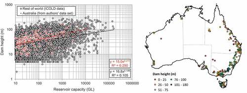
Figure A2. Relationship between reservoir capacity and ratio of reservoir surface area to catchment area comparing 184 Australian reservoirs with 3505 from the rest of world.

References

- ABS (Australian Bureau of Statistics). 2008. “Water and the Murray-Darling Basin – A Statistical Profile, 2000-01 to 2005-06. 4610.0.55.007, 2008”. Accessed 15 August 2008. http://www.abs.gov.au/ausstats/[email protected]/Latestproducts/4D07326348788498CA2574A50014B975?opendocument
- ANCOLD (Australian National Committee on Large Dams). 1994. Guidelines on Dam Safety Management. Australia: Australian National Committee on Dams.
- ANCOLD (Australian National Committee on Large Dams). 2000. Guidelines on Selection of Acceptable Flood Capacity for Dams. Australia: Australian National Committee on Dams.
- ANCOLD (Australian National Committee on Large Dams). 2010. “Register of Large Dams in Australia.” Accesed 20 October 2011 https://www.ancold.org.au/?page_id=24
- Anderson, TW, and DA. Darling. 1952. “Asymptotic Theory Of Certain 'Goodness-of-fit' Criteria Based on Stochastic Processes.” Annals Of Mathematical Statistics 23: 193–212. doi:10.1214/aoms/1177729437.
- Australian Geographic. 2008. “To Dam or Not to Dam. By Peter Meredith.” Australian Geographic Magazine. Accesed May 2017. http://www.australiangeographic.com.au/topics/science-environment/2011/01/to-dam-or-not-to-dam
- Barber, M., and S. Jackson. 2011. Indigenous Water Values and Water Planning in the Upper Roper River, Northern Territory. CSIRO: Water for a Healthy Country National Research Flagship.
- Baumgartner, A., and E. Reichel. 1975. The World Water Balance: Mean Annual Global, Continental and Maritime Precipitation and Runoff. Amsterdam: Elsevier Scientific Publishing Company.
- BoM (Bureau of Meteorology). 2012. Australian Water Resources Assessment 2012. Australian Bureau of Meteorology.
- Cole, B. 2000. “Chapter 1: Dams to the Rescue.” In ‘Dam Technology in Australia 1850-1999ʹ, edited by B. Cole. Australia: Australian National Committee on Large Dams Inc.
- Cole, B. 2003. Australia’s 500 Large Dams, Conserving Water on a Dry Continent. Australia: Australian National Committee on Large Dams Inc.
- Conversation, T. 2011. “Murray Darling Basin Plan Draft Released: Expert Reactions.” Accesed 11 January 2011. http://theconversation.com/murray-darling-basin-plan-draft-released-expert-reactions-4478
- CSIRO, Ian Prosser, Editor. 2011. Water: Science and Solutions for Australia. Melbourne: CSIRO Publishing.
- Department of Agriculture and Water Resources (DAWR). 2016. “National Water Infrastructure Development Fund – Capital Component. Expression of Interest Guidelines.” Department of Agriculture and Water Resources, Australian Government. Accesed. 5 May 2017. https://www.internationalrivers.org/sites/default/files/attached-files/truecostofhydro_en_small.pdf on 5 May 2017
- Doherty, J. 1999. “Gravity Dams.” Chapter 4 in A History of Dam Technology in Australia 1850 – 1999, edited by B. Cole. Institution of Engineers, Australia and Australian National Committee on Large Dams.
- Eagles, J. 2000. “Rockfill Dams with Earth Cores.” Chapter 8 in Dam Technology in Australia 1850 – 1999, edited by B. Cole. 248pp, Penrith, N.S.W: Australian National Committee on Large Dams Inc.
- Forbes, B. A., and M. G. Delaney. 1985. “Design and Construction of Copperfield River Gorge Dam.” Australian National Committee on Large Dams Bulletin 71: 25–41.
- Francou, J., and J. Rodier. 1967. “Essai de classification des crues maximales observées dans le monde.” Cahiers ORSTOM, Série Hydrologie IV (3): 19–46.
- Gehin. 1961. Trans. 7th International Congress on Large Dams, Rome, 3. doi:10.1021/jm50016a012.
- Hutchinson, M. F., J. L. Stein, J. A. Stein, H. Anderson, and P. K. Tickle, 2008. “GEODATA 90 Second DEM and D8: Digital Elevation Model Version 3 and Flow Direction Grid 2008.” Metadata file identifier: a05f7892-d78f-7506-e044-00144fdd4fa6. Accesed March 2011. http://www.ga.gov.au/metadata-gateway/metadata/record/gcat_66006
- ICOLD (International Commission on Large Dams). 2011. “Registre des Barrages – 2011.” Accesed 2 February 2015. http://www.icold-cigb.org/GB/icold/icold.asp
- International Rivers. 2015. “True Cost of Hydropower in China.” Accesed 5 May 2017. https://www.internationalrivers.org/sites/default/files/attached-files/truecostofhydro_en_small.pdf
- Jeffrey, S. J., J. O. Carter, K. M. Moodie, and A. R. Beswick. 2001. “Using Spatial Interpolation to Construct a Comprehensive Archive of Australian Climate Data.” Environmental Modelling & Software 16 (4): 309–330. doi:10.1016/S1364-8152(01)00008-1.
- Kenny, B. C. 1982. “Beware of Spurious Self-correlations!” Water Resources Research 18 (4): 1041–1048. doi:10.1029/WR018i004p01041.
- Kinstler, F. 2000a. “Buttress Dams.” Chapter 7 in Dam Technology in Australia 1850–1999, edited by B. Cole. 248pp, Penrith, N.S.W: Australian National Committee on Large Dams Inc.
- Kinstler, F. 2000b. “Spillways.” In Dam Technology in Australia 1850-1999, edited by B. Cole. 248pp, Penrith, N.S.W: Australian National Committee on Large Dams Inc.
- McMahon, T. A., and A. Adeloye. 2005. Water Resources Yield, 220. CO, USA: Water Resources Publications.
- McMahon, T. A., B. L. Finlayson, A. T. Haines, and R. Srikanthan. 1992. Global Runoff – Continental Comparisons of Annual Flows and Peak Discharges. Germany: Catena Paperback, Catena Verlag.
- McMahon, T. A., R. M. Vogel, G. G. S. Pegram, M. C. Peel, and D. Etkin. 2007. “Global Hydrology – Part 2, Reservoir Storage-yield Performance.” Journal of Hydrology 347 (3–4): 260–271. doi:10.1016/j.jhydrol.2007.09.021.
- Nathan, R. J., and P. E. Weinmann. 2004. “An Improved Framework for the Characterisation of Extreme Floods and for the Assessment of Dam Safety.” Hydrology: Science & Practice for the 21st Century, London, Proc. British Hydrol. Soc. 1: 186–193.
- Nathan, R. J., P. E. Weinmann, and S. A. Gato, 1994. “A Quick Method for Estimating the Probable Maximum Flood in South Eastern Australia.” Water Down Under ’94, Adelaide, Australia, 21–25 November 1994.
- O’Donnell, E., and B. Hart, 2016. “Damming Northern Australia: We Need to Learn Hard Lessons from the South.” The Conversation. Accesed 5 May 2017. https://theconversation.com/damming-northern-australia-we-need-to-learn-hard-lessons-from-the-south-53885
- Peel, M. C., T. A. McMahon, and B. L. Finlayson. 2004. “Continental Differences in the Variability of Annual Runoff – Update and Reassessment.” Journal of Hydrology 295: 185–197. doi:10.1016/j.jhydrol.2004.03.004.
- Petheram, C., J. Gallant, P. Wilson, P. Stone, G. Eades, L. Roger, A. Read, et al., 2014. “Northern Rivers and Dams: A Preliminary Assessment of Surface Water Storage Potential for Northern Australia, CSIRO Land and Water Flagship Technical Report.” Australia: CSIRO. Accesed 10 February 2018 https://publications.csiro.au/rpr/pub?pid=csiro:EP147168
- Petheram, C., L. Rogers, G. Eades, S. Marvanek, J. Gallant, A. Read, B. Sherman, et al., 2013. “Assessment of Surface Water Storage Options in the Flinders and Gilbert Catchments, A Technical Report to the Australian Government from the CSIRO Flinders and Gilbert Agricultural Resource Assessment, Part of the North Queensland Irrigated Agriculture Strategy.” CSIRO Water for a Healthy Country and Sustainable Agriculture flagships. Australia. Accesed 10 February 2018. https://publications.csiro.au/rpr/pub?pid=csiro:EP139850
- Petheram, C., P. Rustomji, T. R. McVicar, W. Cai, F. H. S. Chiew, J. Vleeshouwer, T. G. Van Niel, et al. 2012. “Estimating the Impact of Projected Climate Change on Runoff across the Tropical Savannas and Semiarid Rangelands of Northern Australia.” Journal of Hydrometeorology 13: 483–503. doi:10.1175/JHM-D-11-062.1.
- Petheram, C., and T. A. McMahon. 2019. “Dams, Dam Costs and Damnable Cost Overruns.” Journal of Hydrology X 3: 100026. doi:10.1016/j.hydroa.2019.100026.
- Petheram, C., T. A. McMahon, and M. C. Peel. 2008. “Flow Characteristics of Rivers in Northern Australia: Implications for Development.” Journal of Hydrology 58 (1–2): 93–111. doi:10.1016/j.jhydrol.2008.05.008.
- PMC (Prime Minister and Cabinet), 2015. “Our North, Our Future: White Paper on Developing Northern Australia, Prime Minister and Cabinet.” Commonwealth Government of Australia. Accesed 30 June 2015 https://northernaustralia.dpmc.gov.au/sites/default/files/papers/northern_australia_white_paper.pdf
- Rodier, J., and M. Roche. 1984. World Catalogue of Maximum Observed Floods, 143. International Association of Hydrologic Sciences Publication.
- Schnitter, N.J. 1994. A history of dams: the useful pyramids. AA Balkema, Rotterdam. 266pp.
- Snowy Hydro, 2018. “The Snowy Mountains Scheme: A Civil Engineering Wonder.” Accesed 6 March 2018 https://www.snowyhydro.com.au/our-energy/hydro/the-scheme/on
- Vaze, J., N. Viney, M. Stenson, L. Renzullo, A. Van Dijk, D. Dutta, R. Crosbie, et al., 2013. “The Australian Water Resource Assessment System (AWRA).” Proceedings, 20th International Congress on Modelling and Simulation (MODSIM2013), Adelaide, Australia.
- Watt, B. 2000. “Earthfill Dams.” Chapter 6 in Dam Technology in Australia 1850 – 1999, edited by B. Cole. Australian National Committee on Large Dams Inc.
- WCD (World Commission on Dams). 2000. Dams and Development: A New Framework for Decision-making. World Commission on Dams. London: Earthscan Publications Ltd.
- Zarfl, C., A. E. Lumsdon, J. Berlekamp, L. Tydecks, and K. Tockner. 2015. “A Global Boom in Hydropower Dam Construction.” Aquatic Sciences 77: 161–170. doi:10.1007/s00027-014-0377-0.
Appendix
summarises the number and types of variables available for detailed analyses of the Australian data in which dam height and dam length are related to at-site, catchment, climate, and hydrology attributes. These attributes or variables are detailed in –. Of the 133 attributes, 112 are primary cardinal attributes, 13 are secondary cardinal attributes and 8 are nominal attributes. Dam and reservoir details were obtained from the ANCOLD database. Where erroneous values were identified they were either corrected, if authoritative information were available (i.e. a published study) or removed from the analysis.