The SWTools R package for SILO data acquisition, homogeneity testing and correction

ABSTRACT

Rainfall is a fundamental input to water resources models. Data products are making rainfall data available in application ready formats. There is a temptation to adopt these datasets directly without undertaking thorough quality assurance checks. The SWTools R package is introduced to download, summarise, check and, if necessary, correct rainfall data from a commonly used data product in Australia, the SILO database. A case study is presented where interpolation to extend a dataset after a station closed introduced non-homogeneity when compared to adjacent sites. SWTools functions are used to identify this change and apply corrections to the data. Calibrating a rainfall–runoff model to the datasets with and without corrections had a substantial influence on the simulated water availability in the catchment, with a 30% reduction in average runoff after the rainfall corrections. This case study highlights the importance of undertaking data quality assurance checks, particularly when applying a model outside the calibration period.

KEYWORDS:

• Non-homogeneity test
• SILO
• rainfall

1. Introduction

Rainfall is a primary data input for almost all water resources projects (Black et al. 2011; Vaze et al. 2011). Often these data must be regular, continuous and complete over the period of interest to be used as model inputs. Frequently, the recorded data does not meet these requirements for a range of reasons, including infrequent reading of rainfall gauges resulting in accumulated rainfall totals over time, instrument failure, maintenance, communication issues or the stations being commissioned or decommissioned within the application period. These issues can reduce rainfall data quality which has been well documented to have a large impact on both the parameter values and overall quality of hydrologic model simulations (Andréassian et al. 2001; Oudin et al. 2006; Vaze et al. 2011).

Beyond the most obvious gaps in data that prevent the data being used directly, there can be other errors or inconsistencies in climate data, which present as heterogeneous changes in one data set compared to another at a point in time. Examples include different collection methods (individuals reading a gauge or change in instrumentation), a change in the location or housing used around the instruments, or interference through poor site selection or changes over time due to vegetation growth or infrastructure construction (Lavery, Kariko, and Nicholls 1992). Traditionally, significant effort was required to ensure input data were suitable before modelling could commence. This could involve checking data consistency with other sites, as well identifying suitable sites to infill or correct data, based on spatial proximity, elevation or isohyets.

Climate data products have become readily available that provide application ready data, with any spatial and temporal gaps in data interpolated. Examples of daily rainfall data products in Australia include the Scientific Information for Land Owners (SILO) database (Jeffrey et al. 2001) and Australian Water Availability Project (AWAP) dataset (Jones, Wang, and Fawcett 2009), and global datasets include the NCEP/NCAR Global Reanalysis Product (Kalnay et al. 1996) and CPC Global Unified Gauge-Based Analysis of Daily Precipitation (Chen et al. 2008). Depending on the methodology, these datasets can produce different statistics over a given region and the areal average rainfall calculated is dependent on the density of the rainfall stations (Lee, Kim, and Jun 2018).

One commonly used point-based data set in Australia is the SILO Patched Point Dataset (PPD) (Jeffrey et al. 2001). This dataset consists of observational records at rainfall stations which have been supplemented by interpolated estimates when observed data are missing. This has the significant advantage of addressing many of the issues with rainfall data in a consistent and repeatable way, disaggregating rainfall totals that have accumulated over several days, and infilling gaps through spatial interpolations from other stations. Quality codes are provided to allow the user to determine the source and quality of the values presented. However, often these codes are not checked, and there is a temptation to acquire the data and directly continue to use them in the application of interest.

In using this data over time, applications where interpolated data have materially impacted on water resource assessments have been identified. Without appropriate review of input data to a modelling application, these issues require time-consuming interrogations of all aspects of hydrological modelling, if they are identified in the first place. This paper presents an R package, SWTools, which was developed to acquire SILO PPD for hydrological analyses, allow for interrogation of the source and homogeneity of SILO data, and, if necessary, apply corrections based on other sites. The analyses are based on the original rainfall station data as provided by the Australian Bureau of Meteorology, and hence the results are relevant to other products based on this source datum, e.g. AWAP, which also has an R package to acquire this gridded datum, AWAPer (Peterson et al. 2020). The SWTools package is readily available to R users through The Comprehensive R Archive Network (R Core Team 2021). A case study is presented where SWTools functions are used to review the data quality, identify heterogeneous changes in data from a number of stations, correct this change, and apply the revised rainfall data to simulate the streamflow in a catchment.

2. Methods

2.1. SWTools package overview

The SWTools package has a range of functions for locating, downloading, querying and correcting SILO PPD (summarised in Table 1). Full documentation of the usage of each function is provided with the SWTools package. The functions allow sites within a location to be identified (SILOSitesfromPolygon()) datasets to be retrieved using the SILO Application Programming Interface (API) (SILODownload()), read the downloaded datasets into the R environment (SILOLoad()), summarise the stations locations and data (SILOSiteSummary() and SILOMonthlyRainfall()), review the period of observed data and infilling techniques (SILOSiteSummary(), SILOQualityCodes() and SILOMortonCodes()) and finally undertake homogeneity tests and corrections if necessary (SILOCheckConsistency() and SILOCorrectSite() respectively). SILOReport() can be used to write all summary information and homogeneity test results in a convenient word document.

Table 1. Summary of SILO-related functions in SWTools package.

Function	Usage
SILOSitesfromPolygon	Locate stations within a buffer distance of a polygon shapefile (e.g. catchment boundary)
SILODownload	Downloaded SILO climate files
SILOLoad	Load SILO climate files into a list in the R environment
SILOSiteSummary	Produce a table summarising SILO sites, including station name and number, longitude, latitude, elevation, mean annual rainfall, percentage of data missing
SILOMap	Plot a simple map of the station locations, useful to check stations are in the region intended
SILOThiessenShp	Generate an ESRI shapefile containing Theissen polygons based on the rainfall station locations, and calculate area based weightings
SILOMonthlyRainfall	Boxplots of monthly rainfall with a line of mean monthly evapotranspiration for each site
SILOQualityCodes	Plot the rainfall quality codes for each station in the list
SILOMortonCodes	Plot the quality codes of the input data for Morton’s evaporation calculations, i.e. maximum and minimum temperature, solar radiation and vapor pressure. Evaporation is also plotted, if the site has pan observations
SILOCheckConsistency	Apply two homogeneity tests for each station in the list of SILO sites
SILOCorrectSite	If SILOCheckConsistency() suggests a change in rainfall at a point in time at a site, this function uses linear relationships to correct the change
SILOReport	Generate a word document containing summary information for the sites in the R environment from SILOLoad(). This report includes the output of SILOSiteSummary(), SILOMap(), SILOMonthlyRainfall(), SILOQualityCodes(), SILOMortonCodes() and SILOCheckConsistency()

2.2. Homogeneity tests

Two traditional homogeneity tests have been implemented in SWTools which have been available to hydrologists and data users for close to a century (Merriam 1937). The first is the method of cumulative residuals (e.g. Allen et al. 1998), and the second a double mass analysis (e.g. Chang and Lee 1974). These approaches have been recommended for testing daily rainfall data (e.g. Nathan and McMahon 2017), however further testing of rainfall intensity may be necessary if rainfall at the sub-daily event scale is required for a given application (Wasko et al. 2022).

The tests are applied to annual rainfall totals for each station in the list of station data, Y, and compared to the annual average rainfall from all stations in the list, X_av. This average data set is used to represent a regional homogenous data set for comparison (Allen et al. 1998). It is assumed that the list of station data loaded into the R environment with SILOLoad() contains only stations from the same climatic region where the same trends would be expected.

2.2.1. Cumulative residuals method

This test utilises results from residuals between Y and the linear regression of Y on X_av, with a fixed intercept of 0. If the residuals from the regression are independent random variables (i.e. they exhibit homoscedasticity), then the residuals, ε, follow a normal distribution with mean zero and standard deviation, ${\sigma }_{\mathit{Y}|Xav}$, i.e. $\mathit{\epsilon }\in \mathit{N}\left(0,{\sigma }_{\mathit{Y}|Xav}\right)$ SILOCheckConsistency() produces a scatter plot of Y against X_av to visually inspect the homoscedasticity assumption.

The probability that the cumulative residuals exceed a value over the period of record can be represented by an ellipse with axes α and β, computed as (Allen et al. 1998):

$\mathit{\alpha }=\mathit{n}/2$

$\mathit{\beta }=\frac{n}{{\left(\mathit{n}-1\right)}^{1/2}}{Z}_p{\sigma }_{\mathit{Y}|X}$

Where n is the number of years in the data record and $Z_p$ is the standard normal variate for a given probability of non-exceedance. SILOCheckConsistency() plots probability limits for the 80^th $\left(Z_p=0.84\right)$ and 95^th $\left(Z_p=1.64\right)$ percentile over the cumulative residuals of Y against the linear regression of Y on X_av for each year in the record.

2.2.2. Double mass method

A double mass analysis is a common approach to check consistency over time between two data sets based on the cumulative sum of values in each data set, and is recommended to be included in reporting of hydrological applications (Nathan and McMahon 2017). If Y is homogeneous relative to X_av then the cumulative sum of values, Y_sum and X_av,sum, will follow a straight line. If there is a breakpoint in the line between Y and X_av this suggests Y (assuming X_av is homogenous) is heterogeneous and there is a change in the dataset at the time of the breakpoint. To identify a breakpoint, SILOCheckConsistency() uses the segmented() function from the segmented R package (Muggeo 2008). The method identifies the location of a breakpoint in a dataset compared to the linear regression (see Muggeo 2003), and a bootstrap method is used to escape local minima and represent the uncertainty in the location of any breakpoint (Wood 2001).

SILOCheckConsistency() produces the double mass curve, with the colour scale representing the median quality code for each year, using the same legend as SILOQualityCodes(). The plot also includes the location of any breakpoint on the double mass plot, the confidence limits on the location of the breakpoint, the magnitude of the change in slope between Y_sum and X_av,sum after the breakpoint, and the probability (p value) that the hypothesis that there is no change in slope can be rejected. SILOCheckConsistency() has optional arguments for maximum p value and minimum magnitude of change in slope required to plot a breakpoint on the double mass curve, with defaults of p = 0.05 and a change in slope of 2.5%. The final plot produced by SILOCheckConsistency() is the residuals of Y_sum from the linear regression of Y_sum on X_av,sum against time, to provide a visual representation of the timing of any breakpoint in the linear relationship between Y_sum and X_av,sum.

2.3. Non-homogeneity corrections

If after applying SILOCheckConsistency(), a modeller decides that a given Y is heterogeneous compared to X_av, SILOCorrectSite() can be used to adjust the relationship between Y and a selected second rainfall site, X, after (or before) a point in time. One rainfall site is used for the correction instead of the average of sites used for testing, as after testing information on high-quality stations, that have a long period of observed data, are homogenous compared to the average of sites, and have a similar elevation, annual average rainfall and slope compared to the average of sites to Y can be identified, and hence more likely to represent similar climate conditions.

The correction methodology follows the method of cumulative residuals of Allen et al. (1998). Given two periods of annual rainfall data, $\mathit{k}\in \left[1,2\right]$, around an identified breakpoint, the regression of Y_k on X_k for both periods is computed. For each year in the period to be corrected, j, an annual rainfall correction is computed as the difference between the totals predicted from the two regression equations, Y_2,j and Y_1,j, for X_j, as ΔY = Y_2,j – Y_1,j. To correct the daily rainfall data, a scaling fraction $\mathit{f}=\left(Y_j+\mathrm{\Delta }\mathit{Y}\right)/Y_j$ is applied to each daily value for year j. The start and end years for each period can be specified in SILOCorrectSite(), or by default the full data record is used.

2.4. Application to North Para River rainfall–runoff model

The methods outlined above have been applied to rainfall stations in a case study catchment. This case study also demonstrates the different results that can be produced by a rainfall–runoff model calibrated to rainfall data both pre- and post-correction of heterogeneous changes.

2.4.1. Catchment and data description

The catchment contributing to streamflow station A4260517, North Para River at Penrice, in the Barossa Valley in South Australia has been used as a case study catchment. The station commenced in 1977 and remains open, and is a Bureau of Meteorology Hydrological Reference Station (Zhang et al. 2016), indicating a well-maintained station with a verified rating table, and in an unregulated catchment with minimal land-use change. The catchment area is 117 km² with average annual runoff of 38 mm/year with a seasonal flow regime, typically between May and December each year. The Mediterranean climate has mean annual rainfall varying from 480 mm at the station to 720 mm in the headwater catchments. The predominant land use in the headwaters is viticulture, making way for grazing in the lower sub-catchments, with farm dam densities (volume of storage/catchment area) aligned to this land use, ranging from 35 ML/km² in the upper catchment to 4 ML/km² lower in the catchment (Jones-Gill and Savadamuthu 2014).

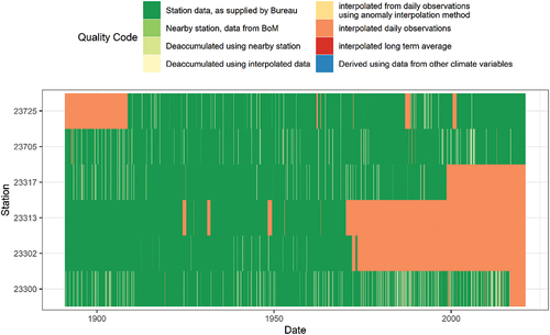
Figure 1 provides a map of the catchment, including the location of available SILO rainfall stations. A summary of the stations, produced by SILOReport(), is provided as supplementary material. The one station within the catchment, 23302, as well as the station closest to the high rainfall headwater catchments, 23313, have a long period of record, commencing in 1870s; however, they were closed in 1975 and 1970, respectively, as seen from the quality codes produced by SILOQualityCodes() (Figure 2). Hence, the rainfall and streamflow records do not overlap for these stations. Homogeneity tests outlined in Section 2.2 were applied to all stations in Figure 1, where it was identified that corrections were required to be applied for stations 23302 and 23313 for the period of interpolated data after the stations were closed. Further details are presented in the Results section.

Figure 1. Map of the catchment contributing to station A5050517 and rainfall stations within and near the catchment. Rainfall site 23705 is 20 km to the south, at a similar elevation and annual rainfall to site 23313.

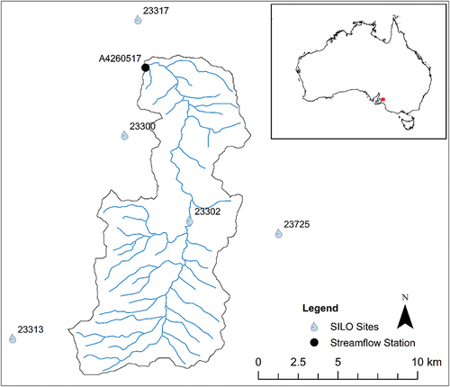
Figure 2. Rainfall data quality codes for the stations available for the case study catchment, produced by SILOQualityCodes(). Interpolated daily observations (orange) indicates where spatial interpolation has been used to infill the data record, or to extend the data record in the case of closed stations.

2.4.2. Rainfall–runoff model

A rainfall–runoff model has been calibrated to each of the input datasets. The first model applied rainfall data directly from SILO (‘Original’) and the second model applied rainfall data, after detecting heterogeneous periods in the rainfall data compared to the regional average and then correcting the data in those periods (‘Corrected’). Thiessen polygons were used to calculate the spatially weighted average of the station data as input to the rainfall runoff model for rainfall and potential evapotranspiration (PET), with the weightings produced by SILOThiessenShp(). The PET input was the Morton’s wet-environment areal potential evapotranspiration over land formulation (Morton 1983) available from SILO.

GR6J was selected as the rainfall runoff model, an extension to the commonly used GR4J model (Perrin, Michel, and Andréassian 2003) with a focus on improvement in the representation of the low flows through an additional routing store (Pushpalatha et al. 2011). This was considered necessary as low flows are an important component of the flow regime ecologically for this catchment (Jones-Gill and Savadamuthu 2014). The implementation of GR6J in the airGR package was used (Coron et al. 2017).

The model was calibrated to the square root transform of the daily flows, to increase the focus on the overall flow regime. The objective function was the modified Kling-Gupta Efficiency (KGE) (Kling, Fuchs, and Paulin 2012) using the calibration method developed by Michel (1991), available in airGR. After transforming the parameter space to similar ranges, this calibration method applies an initial grid-based screening of the global parameter space to identify suitable starting values for a steepest descent local search algorithm. The deterministic algorithm produces a consistent calibration approach to compare results from the two rainfall inputs, and the pseudo-local calibration method was deemed suitable for calibration of this parsimonious rainfall runoff model with six calibration parameters.

Three different periods were considered. The calibration period (1/1/1978–31/12/2004) was used to determine values for the six model parameters for each rainfall input dataset. The validation period was used to test the generalisability of the model, if similar model performance is achieved compared to streamflow data that was not used in the calibration of the model parameters (1/1/2005–31/12/2020). The application period was used to represent a use case for the model, where the model is used to simulate streamflow prior to the observed record becoming available (1/1/1891–31/12/1977). For example, the application period outputs may be used to represent a wider variety of climatic conditions and calculate more robust streamflow statistics (based on a larger sample) to inform the setting of water extraction limits. The application period was used to test if corrections to the rainfall data to improve the homogeneity between rainfall stations had an impact on the simulated water available in the application period.

3. Results

3.1. Homogeneity tests

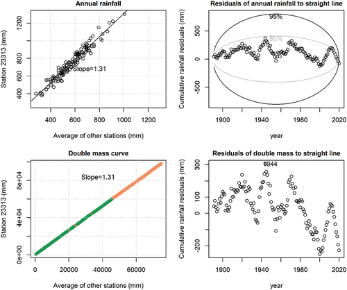
SILOCheckConsistency() was applied to the SILO data for the six stations (shown in Figures 1 and 2). Results for two of the stations are presented in Figures 3 and 4, with all results for all stations provided as Supplementary Material. Station 23,313 is near the wetter headwaters of the catchment, as indicated by the slope of 1.26 between the annual rainfall totals (top left plot in Figure 3). The cumulative residuals from the annual rainfall to this straight line indicate a non-homogeneous change around 1970, which is statistically significant at greater than the 95^th percentile. A breakpoint was also identified in the double mass curve, which coincides with the closing of the station, and a reduction in slope at this time of 0.135. Upon assessment of the results in Figure 3, it was decided to correct the interpolated data from 1970 onwards.

Figure 3. Homogeneity tests from SILOCheckConsistency() for station 23313. The outputs suggest the interpolated data (orange points in double mass curve panel) are significantly different to the observed data (green) with a reduction in slope of 13.5% and significant p value (p<<0.05). The residuals of annual rainfall to straight line panel also supports this discontinuity, with the cumulative residuals over 1000 mm outside the 95^th percentile ellipse, with the peak also coinciding with the closing of the site in 1970.

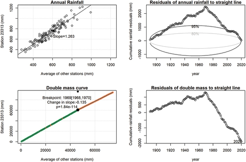
Figure 4. Homogeneity tests from SILOCheckConisistency() for station 23705. For this site, the breakpoint analysis did not identify a statistically significant change in slope. The residuals of annual rainfall to straight line panel deviate beyond the 80^th percentile confidence level for only a small number of years. Based on these results, this site was deemed to have homogeneous data throughout the record.

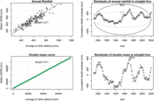
Stations in the region with similar annual rainfall and elevation were interrogated to find a suitable site to correct station 23313. Station 23705 was identified as having a similar relationship to the average of stations (slope of 1.21 in Figure 4), the cumulative annual residuals remain within the 95^th percentile ellipse (and 80^th percentile ellipse) for much of the time, and no breakpoint was identified on the double mass curve (Figure 4). Station 22302 in the centre of the catchment was also found to have a non-homogenous change at the time when the station closed (see Supplementary Material) and was corrected with station 23725 using the relationship based on data from the time that station 23725 opened (1908) and the breakpoint in 1973.

3.2. Non-homogeneity corrections

SILOCorrectSite() was used to correct the rainfall data for site 23313 and 23302 for the period of interpolated data. The increase in station 23313 annual rainfall based on that recorded at station 23705 was computed as the difference between the red and blue linear regression lines in Figure 5, with the new annual rainfall total used to calculate a fraction to scale the daily rainfall for that year. This methodology is implemented in the SILOCorrectSite() function, which also produced Figure 5. The homogeneity tests were again applied to the data for station 23313, this time after correction, and from Figure 6, the adjusted data now pass the two tests, with the cumulative annual residuals remaining within the 80^th percentile confidence limits, and no breakpoint on the double mass curve identified. The mean annual rainfall for station 23313 in the period of correction (1970–2020) increased from 655 mm to 732 mm, and for station 23302 (period of correction 1973–2020) from 550 mm to 589 mm.

Figure 5. Annual rainfall totals for two rainfall stations near the study catchment. The linear regression lines were used to correct rainfall data for station 23313 (produced by SILOCorrectSite()). The trend line for the second period (blue) is scaled up to match the relationship between stations for the period with homogeneous data (red line) to correct for the non-homogeneity identified in Figure 3.

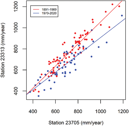
Figure 6. Homogeneity tests from SILOCheckConisistency function for station 23313 after applying SILOCorrectSite function for station 23313 based on station 23705 for the interpolated data after 1970. In contrast to Figure 3, now the interpolated data are consistent with the observed data prior to 1970, as indicated by the constant slope in the double mass curve panel, and cumulative residuals within the 80^th percentile ellipse (top right).

3.3. Rainfall–runoff model

3.3.1. Model calibration

The results from the model calibration are provided in Table 2, including the KGE and Nash-Sutcliffe Efficiency values and the mean annual rainfall and streamflow for the different periods considered. Both models accurately represent the observed mean annual streamflow over the calibration period, 46.6 mm/year. The selection of the GR6J model appears appropriate, with acceptable KGE and NSE values; however, there is some reduction in performance in the validation period, most likely due to overestimation of the observed streamflow (observed 23.8 mm/year) for this drier period. The model performance is similar for the two rainfall data sets, with slightly better metrics values for the corrected rainfall data. The calibrated parameter values for the rainfall–runoff model (Table 3) indicate a higher X1 value, requiring more rainfall for the production store to fill and produce direct runoff, was necessary to lose more water from the catchment and simulate the same streamflow for the corrected rainfall compared to the original rainfall.

Table 2. Results from the rainfall runoff model for streamflow station A5050517, including Kling–Gupta Efficiency (KGE), Nash–Sutcliffe Efficiency (NSE) values for the calibration and validation periods, based on both the original SILO rainfall data (‘Original’), and the rainfall data corrected for non-homogeneity (‘Corrected’). The mean annual rainfall (P) and simulated streamflow (Q) for both rainfall datasets and each period are also provided.

Period	Rainfall data	$\mathit{KGE}\left(\sqrt{\mathit{Q}}\right)$	$\mathit{NSE}\left(\sqrt{\mathit{Q}}\right)$	Mean P (mm/yr)	Mean Q (mm/yr)
Calibration	Original	0.89	0.79	562	45.3
	Corrected	0.9	0.81	595	45.7
Validation	Original	0.44	0.61	521	26.9
	Corrected	0.45	0.64	554	27.3
Application	Original	No observed flow data		612	60.2
	Corrected			615	49.2

Table 3. Calibrated GR6J model parameters based on both the original SILO rainfall data (‘Original’), and the rainfall data corrected for non-homogeneity (‘Corrected’).

Climate data	X1	X2	X3	X4	X5	X6
	(mm)	(mm/d)	(mm)	(days)	(-)	(mm)
Original	212	−0.44	15.54	1.32	0.07	0.14
Corrected	254	−0.46	13.23	1.31	0.07	0.28

3.3.2. Model application

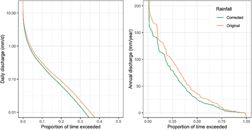
The model calibrated to each rainfall data set was applied to the available climate data prior to model calibration, from 1891 to 1977. The rainfall data are the same for most of this period, with corrections to site 23,313 resulting in corrected rainfall data after 1970. Exceedance curves of the daily and annual discharge (Figure 7) indicate that the model based on the corrected rainfall data simulates substantially less streamflow over the long term, with a mean annual runoff of 49 mm/year compared to 60 mm/year, 22% less water available as a long-term average (Table 2). There is also a reduction in the proportion of days with flow, reducing from 35% of the time to 32% (based on a flow threshold of 0.01 mm/d). These differences are potentially significant in the context of setting water allocations and environmental water requirements in the catchment and demonstrate the implications of extrapolating model results based on inputs that are not consistent over the modelling period.

Figure 7. Exceedance curve of daily (left) and annual discharge (right) over the period prior to model calibration (1891–1977) for the rainfall runoff models calibrated to the original and corrected rainfall data.

4. Discussion

The software contribution of the SWTools package provides a simple, fast and readily available framework for the Australian hydrological community to undertake rainfall data homogeneity checks from a commonly used database. The software provides a repeatable and well-accepted methodology to apply corrections to rainfall data if deemed necessary by the modeller and provides a standard report to support model documentation. The functions available can be applied to other data sources that are read into the R environment with the same data structure as that created by SILOLoad() (the SILOLoad() documentation provides details of the data structure). The code is open source (GNU General Public Licence V3) and as such the package represents a starting point for the community to add additional data sources and functionality as required.

While the broad methodology implemented in the SWTools package is not new, the specific implementation of the more advanced breakpoint estimation method is novel to the water resources field. The breakpoint analysis implemented in SWTools currently identifies one breakpoint if it exists, where it is conceivable that there could be more than one change in the relationship between rainfall at one site and the regional average in some cases. The functions available could be extended to the identification of multiple breakpoints. Currently, if an initial application of SILOCheckConsistency() suggests that more than one breakpoint might exist, this can be tested by adjusting the start and end dates of the data considered to assess each period incrementally.

The analysis of SILO PPD found the interpolated data extending the rainfall record after stations closed underestimated the rainfall based on the relationship with adjacent stations. No physical reason for a change in spatial rainfall patterns in the catchment was identified (e.g. large-scale change in land use) and hence the ‘Corrected’ rainfall data, updated to maintain homogeneity with a nearby high-quality rainfall station over the period of record, are expected to be more representative of the rainfall that occurred at locations of stations 23313 and 23302 for the period after the stations were closed. The SILO interpolation algorithm normalises the observed data using a power transformation to minimise persistent variability, such as seasonality and orographic effects (Jeffrey et al. 2001; Richardson 1977). The power value used to normalise the observed data is based on spatially interpolated values, and different values are used for each month (Jeffrey 2006). Reviews have found this approach suitable across Australia with a wide range of climatic regions (Beesley, Frost, and Zajaczkowski 2009; Tozer, Kiem, and Verdon-Kidd 2012). However, for a given local scale application it is the responsibility of the modeller to understand and review the input data available and assess the sensitivity of the application to any data uncertainties.

The case study is an example where rainfall non-homogeneity had a material influence on the simulated water availability. In this case, the modelled relationship between rainfall and runoff was unlikely to represent the underlying processes without homogeneity corrections to the interpolated data. This resulted in a 1288 ML/year increase in mean annual streamflow in the catchment, representing 38% of the total resource capacity (3400 ML/year), similar to the total capacity of licensed farm dams in the catchment (1184 ML), and more than three times greater than the water use in the catchment, estimated to be 34% of the licenced dam capacity (Jones-Gill and Savadamuthu 2014). While the models presented here were not used to inform the Barossa Prescribed Water Resource Area Water Allocation Plan (Adelaide and Mount Lofty Ranges Natural Resources Management Board 2009), this volume difference is significant in the context of water availability and extraction in the catchment, and hence potentially influences the water allocations made available. The persistence of the flow has been found to be a strong predictor of ecological responses in this catchment, and while a reduction of 3% of the time appears small, this is 9% of the flowing period, and may be sufficient to lead to different environmental objectives being set for the catchment. While this is only one example, it is not an outlier and demonstrates the importance of understanding the source of input data and undertaking appropriate quality checks before investing significant effort in developing environmental models.

In the case study presented, it was the closing of a rainfall station that resulted in non-homogeneous changes in rainfall data for the period that was interpolated based on surrounding stations. However, this is not always the case, for example, station 23317 was closed in 1999, but the tests did not identify a change in homogeneity with the other sites for this station. Spatial interpolation of daily data is more likely to be consistent with the historical data in relatively flat terrain with sufficient gauge density, whereas topographic effects are a key reason for changes in rainfall statistics over short distances where the interpolation methods may be less suitable. Some judgement from the modeller may be required to determine if corrections are required, and if this is the case, which period before or after a breakpoint is most likely to be the homogeneous data. In cases where this is less obvious than that in the case study, The Bureau of Meteorology Weather Station Directory provides climatological station metadata including the equipment history to evaluate the data quality and the cause for a perceived change beyond the codes provided by SILO. Some judgement is also required to identify suitable stations to include in the station average for comparison, where the local topography and gauge density are likely to influence the number of stations that are available to be included. Some iteration may be required to remove suspected lower-quality stations from being included in the regional average to evaluate changes in the homogeneity test results.

The issues outlined in this work are not unique to point-based data and are just as, if not more, relevant for gridded products, which in the case of AWAP may not reproduce observed data where available (Tozer, Kiem, and Verdon-Kidd 2012). The functions available in SWTools evaluate potential changes in homogeneity against nearby stations for the station data provided by the Australian Bureau of Meteorology (via SILO), and as such the results are relevant for any product derived from this data (e.g. the SILO gridded dataset or the AWAP dataset (Jones, Wang, and Fawcett 2009)).

Another application where it is important to undertake homogeneity checks is when investigating state changes and non-stationarity detection (e.g. Hughes et al. 2021; Peterson et al. 2021). For the case study presented here, if the rainfall data was not checked, potentially a state change in the rainfall–runoff relationship would be inferred, as the data suggest more streamflow was generated for the same rainfall in the latter period. However, the cause is more likely to be the non-homogenous interpolated rainfall data rather than a true change in processes in the catchment. While not presented in this work, similar effort in the quality assessment of streamflow data is required (e.g. McMahon and Peel 2019), where a change in rating curve or monitoring structure may also imply a change in the relationship between rainfall and runoff.

The accuracy of the potential evapotranspiration (PET) data is often less important for rainfall runoff modelling, particularly in water-limited catchments such as the one used in this study. Many applications use a regular monthly average, given this lower sensitivity and lower variability in PET (Chapman 2003), however this is not always the case (Guo, Westra, and Maier 2017). In applications such as actual water loss from permanent water storage, the influence of the derived PET can be more significant. SWTools includes SILOMortonQualityCodes() function to plot the quality codes for variables that are input to the calculation of the evaporation data available from SILO, similar to Figure 2. For many stations, there are no observed temperature data, for the dry bulb (minimum and maximum temperature) or wet bulb (used to calculate vapour pressure) instruments. Solar radiation data for all stations is derived from a gridded product based on observed cloud cover twice daily (Zajaczkowski, Wong, and Carter 2013). Department for Environment and Water (2021) found that the cloud-cover-derived solar radiation underestimated solar radiation observed from pyranometers by an average of 6%, which in turn led to an average underestimation of Morton’s Lake evaporation by 9%. When undertaking a water balance on a storage where the evaporation loss is a large component, these differences may be substantial and important.

The SWTools package also includes helper functions for working with Australia’s National Hydrological Modelling Platform, eWater Source (Welsh et al. 2013). This includes functions for writing SILO climate data in the format expected by Source, reading Source outputs into the R environment, as well as interacting with Source models via the Veneer plugin. SWTools provides functions that interact with the Veneer API to modify and run a Source model that is open in the graphical user interface, as well as query information about the model and retrieve results from runs that have been undertaken. Finally, SWTools provides functions for downloading and reading data from the Government of South Australia hydrological database (https://water.data.sa.gov.au/, accessed 5/7/2022), which were used to acquire the streamflow data for the case study.

5. Conclusions

Climate, and in particular rainfall, data is a key input to many water resources models. The estimate of rainfall across a region of interest can be influenced by which stations are available at different points in time, as well as the quality of the observed data from those stations. Data products are readily available that provide application ready rainfall data with any gaps in space and time interpolated, and these services provide significant efficiencies for modellers. However, the modeller still has a responsibility to ensure that input data is suitable for the intended purpose.

A case study was presented to provide an example where data interpolation had a material influence on the simulated water availability, where the relationship between rainfall and runoff calibrated for the period with streamflow data available was unlikely to represent the underlying processes without homogeneity corrections to the interpolated data. While this was only one example, it is not an outlier and demonstrates the importance of understanding the source of input data and undertaking appropriate quality checks before investing significant effort in developing environmental models.

The SWTools package was introduced to support this review process for rainfall data from one commonly used data source in Australia, SILO PPD. With a few lines of R code data can be discovered, downloaded, imported, summarised, checked, and if necessary, corrected, for homogeneity with the regional average. Additional importing routines, equivalent to SILOLoad(), could be added to enable the homogeneity checking and correcting routines to be applied to rainfall data from other sources. The code is open source (GNU General Public Licence V3) and as such the package represents a starting point for the community to add additional data sources and functionality as required. The SWTools package also includes functions to support the use of eWater Source hydrological models from R, including writing climate data input files and reading output files, as well as interacting with Source models via the Veneer plugin.

Acknowledgements

Parts of this work were undertaken while some authors were employed by the Department for Environment and Water (DEW), South Australia (MG and MA) and the University of Adelaide (MG). Dr Daniel McCullough (DEW) is thanked for his contribution to the SILOThiessenShp() function. The authors thank the two anonymous reviewers for their constructive comments that improved this manuscript.

Disclosure statement

No potential conflict of interest was reported by the authors.

Data availability statement

The SWTools package is available from the Comprehensive R Archive Network. The Source code and code to produce the analyses in this manuscript are available at https://github.com/matt-s-gibbs/swtools and https://github.com/matt-s-gibbs/Rainfall-homogeneity-example., respectively.

Additional information

Funding

This research did not receive any specific grant from funding agencies in the public, commercial, or not-for-profit sectors.

Notes on contributors

Matt Gibbs

Matt Gibbs is a Senior Research Scientist (hydrologist) in CSIRO’s Water Resource Assessment team. Matt has 15 years’ experience in the fields of water resources, modelling and optimisation techniques based in academia, state and federal government. He has worked extensively on the River Murray, Lower Lakes and Coorong in South Australia, focusing on hydrological, hydraulic and water quality modelling to inform policy, infrastructure, and river operations decisions. Matt has recently published in the fields of river restoration, inundation and hydraulic modelling, environmental water management, uncertainty analysis, streamflow forecasting as well as salinity and blackwater modelling.

Mark Alcorn

Mark Alcorn is a Senior Hydrologist at Jacobs. He has over 15 years’ experience as a hydrologist, with much of this time in state government in South Australia. His main interest is in catchment hydrology, in particular the representation and impact of farm dams on hydrology and implications for water allocation planning.

Jai Vaze

Jai Vaze is an internationally recognised hydrologist developing methods to estimate runoff in ungauged catchments and studying the impacts of land use and climate change on catchment, regional and continental-scale water balance. He is currently a Research Team Leader (Water Resources Assessment Team) within Land and Water Business unit. He collaborates widely with leading scientists from Australian Universities and State Government Departments, and from France, the UK, the USA, Ireland, South Africa, China, Nepal, and India. He has worked (and continues to work) on and led many high impact projects that contribute to key national initiatives including the CSIRO Sustainable Yields projects, the AWRA project, the MDBA floodplain inundation modelling project, the eWater Source, SEACI, the Bioregional Assessments project and the Northern Australian Water Resources Assessment project.

References

- Adelaide and Mount Lofty Ranges Natural Resources Management Board. 2009. “.” In: Water Allocation Plan - Barossa Prescribed Water Resources Area, Eastwood, South Australia: Adelaide and Mount Lofty Ranges Natural Resources Management Board, Government of South Australia.
- Allen, R. G., L. S. Pereira, D. Raes, and M. Smith. 1998. Crop Evapotranspiration: Guidelines for Computing Crop Water Requirements. Rome: Food and Agriculture Organization of the United Nations.
- Andréassian, V., C. Perrin, C. Michel, I. Usart-Sanchez, and J. Lavabre. 2001. “Impact of Imperfect Rainfall Knowledge on the Efficiency and the Parameters of Watershed Models.” Journal of Hydrology 250 (1–4): 206–223. doi:https://doi.org/10.1016/S0022-1694(01)00437-1.
- Beesley, C. A., A. J. Frost, and J. Zajaczkowski 2009 13-17 July 2009. A Comparison of the BAWAP and SILO Spatially Interpolated Daily Rainfall Datasets. Paper presented at the 18th World IMACS Congress and MODSIM09 International Congress on Modelling and Simulation, Cairns, Australia.
- Black, D., P. Wallbrink, P. Jordan, D. Waters, C. Carroll, and J. Blackmore. 2011. Towards Best Practice Model Application - Generic Guidelines for Water Management Modelling. eWater CRC. https://ewater.org.au/document-library/.
- Chang, M., and R. Lee. 1974. “Objective Double-Mass Analysis.” Water Resources Research 10 (6): 1123–1126. doi:10.1029/WR010i006p01123.
- Chapman, T. G. 2003. “Estimation of Evaporation in Rainfall-Runoff Models.” Modsim 2003: International Congress on Modelling and Simulation 1-4: 148–153.
- Chen, M. Y., W. Shi, P. P. Xie, V. B. S. Silva, V. E. Kousky, R. W. Higgins, and J. E. Janowiak. 2008. “Assessing Objective Techniques for Gauge-Based Analyses of Global Daily Precipitation.” Journal of Geophysical Research-Atmospheres 113 (D4): 113(D4. doi:https://doi.org/10.1029/2007JD009132.
- Coron, L., G. Thirel, O. Delaigue, C. Perrin, and V. Andréassian. 2017. “The Suite of Lumped GR Hydrological Models in an R Package.” Environmental Modelling & Software 94: 166–171. doi:10.1016/j.envsoft.2017.05.002.
- Department for Environment and Water. (2021). Methodology for Calculating Flow Through the River Murray barrages. Government of South Australia Through Department for Environment and Water, DEW Technical report 2021/04, Adelaide
- Guo, D., S. Westra, and H. R. Maier. 2017. “Impact of Evapotranspiration Process Representation on Runoff Projections from Conceptual Rainfall-Runoff Models.” Water Resources Research 53 (1): 435–454. doi:10.1002/2016WR019627.
- Hughes, J., N. Potter, L. Zhang, and R. Bridgart. 2021. “Conceptual Model Modification and the Millennium Drought of Southeastern Australia.” Water 13 (5): 669. doi:10.3390/w13050669.
- Jeffrey, S. J. 2006. “.” In Error Analysis for the Interpolation of Monthly Rainfall Used in the Generation of SILO Rainfall Datasets. Indooroopilly, Queensland: Department of Natural Resources and Water.
- Jeffrey, S. J., J. O. Carter, K. B. Moodie, and A. R. Beswick. 2001. “Using Spatial Interpolation to Construct a Comprehensive Archive of Australian Climate Data.” Environmental Modelling & Software 16 (4): 309–330. doi:10.1016/S1364-8152(01)00008-1.
- Jones-Gill, A., and K. Savadamuthu 2014. Hydro-Ecological Investigations to Inform the Barossa PWRA WAP Review – Hydrology Report. Government of South Australia through Department of Environment Water and Natural Resources, Adelaide
- Jones, D. A., W. Wang, and R. Fawcett. 2009. “High-Quality Spatial Climate Data-Sets for Australia.” Australian Meteorological and Oceanographic Journal 58 (4): 233–248. doi:10.22499/2.5804.003.
- Kalnay, E., M. Kanamitsu, R. Kistler, W. Collins, D. Deaven, L. Gandin, M. Iredell, et al. 1996. “The NCEP/NCAR 40-Year Reanalysis Project.” Bulletin of the American Meteorological Society 77 (3): 437–471. doi:10.1175/1520-0477(1996)077<0437:Tnyrp>2.0.Co;2.
- Kling, H., M. Fuchs, and M. Paulin. 2012. “Runoff Conditions in the Upper Danube Basin Under an Ensemble of Climate Change Scenarios.” Journal of Hydrology 424-425: 264–277. doi:10.1016/j.jhydrol.2012.01.011.
- Lavery, B., A. Kariko, and N. Nicholls. 1992. “A Historical Rainfall Data Set for Australia.” Australian Meteorological Magazine 40 (1): 33–39.
- Lee, J., S. Kim, and H. Jun. 2018. “A Study of the Influence of the Spatial Distribution of Rain Gauge Networks on Areal Average Rainfall Calculation.” Water 10 (11): 1635. doi:10.3390/w10111635.
- McMahon, T. A., and M. C. Peel. 2019. “Uncertainty in Stage–Discharge Rating Curves: Application to Australian Hydrologic Reference Stations Data.” Hydrological Sciences Journal 64 (3): 255–275. doi:10.1080/02626667.2019.1577555.
- Merriam, C. F. 1937. “A Comprehensive Study of the Rainfall on the Susquehanna Valley.” Eos Transactions American Geophysical Union 18 (2): 471–476. doi:10.1029/TR018i002p00471.
- Michel, C. 1991. Hydrologie appliquée aux petits bassins ruraux. Antony, France: Cemagref.
- Morton, F. I. 1983. “Operational Estimates of Lake Evaporation.” Journal of Hydrology 66 (1–4): 77–100. doi:10.1016/0022-1694(83)90178-6.
- Muggeo, V. 2008. “Segmented: An R Package to Fit Regression Models with Broken-Line Relationships.” R News 8: 20–25.
- Muggeo, V. M. R. 2003. “Estimating Regression Models with Unknown Break-Points.” Statistics in Medicine 22 (19): 3055–3071. doi:10.1002/sim.1545.
- Nathan, R. J., and T. A. McMahon. 2017. “Recommended Practice for Hydrologic Investigations and Reporting.” Australasian Journal of Water Resources 21 (1): 3–19. doi:10.1080/13241583.2017.1362136.
- Oudin, L., C. Perrin, T. Mathevet, V. Andréassian, and C. Michel. 2006. “Impact of Biased and Randomly Corrupted Inputs on the Efficiency and the Parameters of Watershed Models.” Journal of Hydrology 320 (1–2): 62–83. doi:https://doi.org/10.1016/j.jhydrol.2005.07.016.
- Perrin, C., C. Michel, and V. Andréassian. 2003. “Improvement of a Parsimonious Model for Streamflow Simulation.” Journal of Hydrology 279 (1–4): 275–289. doi:https://doi.org/10.1016/S0022-1694(03)00225-7.
- Peterson, T. J., M. Saft, M. C. Peel, and A. John. 2021. “Watersheds May Not Recover from Drought.” Science 372 (6543): 745–749. doi:10.1126/science.abd5085.
- Peterson, T. J., C. Wasko, M. Saft, and M. C. Peel. 2020. “AWAPer: An R Package for Area Weighted Catchment Daily Meteorological Data Anywhere Within Australia.” Hydrological Processes 34 (5): 1301–1306. doi:10.1002/hyp.13637.
- Pushpalatha, R., C. Perrin, N. Le Moine, T. Mathevet, and V. Andréassian. 2011. “A Downward Structural Sensitivity Analysis of Hydrological Models to Improve Low-Flow Simulation.” Journal of Hydrology 411 (1–2): 66–76. doi:https://doi.org/10.1016/j.jhydrol.2011.09.034.
- R Core Team. 2021. R: A Language and Environment for Statistical Computing. Vienna, Austria: R Foundation for Statistical Computing. https://www.R-project.org/.
- Richardson, C. W. 1977. A Model of Stochastic Structure of Daily Precipitation Over an Area. Hydrology paper no. 91. Fort Collins: Colorado State University.
- Tozer, C. R., A. S. Kiem, and D. C. Verdon-Kidd. 2012. “On the Uncertainties Associated with Using Gridded Rainfall Data as a Proxy for Observed.” Hydrology and Earth System Sciences 16 (5): 1481–1499. doi:10.5194/hess-16-1481-2012.
- Vaze, J., P. Jordan, R. Beecham, A. Frost, and G. Summerell. 2011. Guidelines for Rainfall-Runoff Modelling: Towards Best Practice Model Application. eWater CRC.
- Vaze, J., D. A. Post, F. H. S. Chiew, J. M. Perraud, J. Teng, and N. R. Viney. 2011. “Conceptual Rainfall–Runoff Model Performance with Different Spatial Rainfall Inputs.” Journal of Hydrometeorology 12 (5): 1100–1112. doi:10.1175/2011JHM1340.1.
- Wasko, C., J. B. Visser, R. Nathan, M. Ho, and A. Sharma. 2022. “Automating Rainfall Recording: Ensuring Homogeneity When Instruments Change.” Journal of Hydrology 609: 127758. doi:10.1016/j.jhydrol.2022.127758.
- Welsh, W. D., J. Vaze, D. Dutta, D. Rassam, J. M. Rahman, I. D. Jolly, P. Wallbrink, et al. 2013. “An Integrated Modelling Framework for Regulated River Systems.” Environmental Modelling & Software 39: 81–102. doi:10.1016/j.envsoft.2012.02.022.
- Wood, S. 2001. “Minimizing Model Fitting Objectives That Contain Spurious Local Minima by Bootstrap Restarting.” Biometrics 57 (1): 240–244. doi:10.1111/j.0006-341X.2001.00240.x.
- Zajaczkowski, J., K. Wong, and J. Carter. 2013. “Improved Historical Solar Radiation Gridded Data for Australia.” Environmental Modelling & Software 49: 64–77. doi:10.1016/j.envsoft.2013.06.013.
- Zhang, X. S., G. E. Amirthanathan, M. A. Bari, R. M. Laugesen, D. Shin, D. M. Kent, A. M. MacDonald, M. E. Turner, and N. K. Tuteja. 2016. “How Streamflow Has Changed Across Australia Since the 1950s: Evidence from the Network of Hydrologic Reference Stations.” Hydrology and Earth System Sciences 20 (9): 3947–3965. doi:10.5194/hess-20-3947-2016.