Load distribution factors for quick design and assessment in typical Australian bridges

ABSTRACT

The increase in freight productivity in Australia is pressuring Australian bridge infrastructure. Bridge assessment is crucial to ensure the safety of bridges to accommodate heavier vehicles. Load distribution factor (LDF) has been widely used for bridge design and evaluation in the preliminary stage, but it is not specified in the Australian standard code. This study aims to develop the LDFs for typical Australian bridges with the most adverse load effects of single- and two-lane loads. Later, the LDFs were compared with the LDF equations in the different standards, including National Association of Australian State Road Authorities (National Association of Australian State Road Authorities, 1976), American Association of Highway and Transportation Officials: Load and Resistance Factor Design (AASHTO (2017), Henry’s and modified Henry’s methods. It can be concluded that the AASHTO (2017) LDF equations provide very good correlations with typical Australian bridges. It is possible to use the AASHTO LRFD LDF equations for assessing and designing in Australian concrete I-girder and Super-T girder bridges. However, most AASHTO LFRD provides conservative results of LDFs compared with LDFs of Australian bridges. It is recommended that LDFs of Australian bridges should be developed for bridge design and assessment.

KEYWORDS:

• Load distribution factor
• I-girder
• super-T girder

1. Introduction

Concrete I-girder and Super-T girder bridge decks are prevalent in bridge construction in Victoria, Australia, constituting approximately 30% of the state’s bridge inventory (DataVic 2021). Prestressed concrete I-girders were adopted in Australia before 1976 and have continued to be utilised in bridge construction. In the 1990s, Super-T girders were developed in Australia, gaining widespread adoption not only in Australia but also in New Zealand. They have become a common bridge design in regions such as New South Wales and Victoria.

The Australian national reform agenda, aimed at enhancing freight productivity, has resulted in increased vehicle loads on bridges across the country. With safety as a paramount concern in asset management, bridge evaluation has become essential to ensure the structural integrity of bridges when accommodating newer and heavier vehicles. Various approaches for bridge assessment have been implemented in Australia, including load rating factors, comparative assessments, and comprehensive evaluations. These approaches primarily focus on individual bridge analysis, which necessitates intricate analytical and numerical methods like finite element and grillage analyses. However, assessing each bridge individually through analytical methods can be time-consuming.

Consequently, many countries, including Australia, have turned to the load distribution factor (LDF) to address the limitations of analytical analyses. The LDF offers a way to swiftly estimate live load distribution across the bridge superstructure, enabling the derivation of load demands without the need for extensive analytical analysis. This parameter has significant importance in calculating live load responses and is a fundamental component in the preliminary stages of designing or evaluating superstructures according to the American Association of State Highway and Transportation Officials (AASHTO) guidelines.

The basis for the LDF dates back to the work of Westergaard in 1930 and Newmark in 1938. The AASHTO Standard Specification of Highway Bridges, introduced in 1931, incorporated the LDF method for bridge design, utilising what became known as S-over (S/D) equations, where S represents centre-to-centre girder spacing and D is a constant related to the bridge superstructure type. These straightforward equations, referred to as S-over equations, were also included in the Australian bridge design standard National Association of Australian State Road Authorities (1976). They were employed in designing various Australian bridge types, such as prestressed concrete I-girders, T-beams, spread box beams, and steel grids.

A pivotal advancement was initiated by Zokaie et al. (1991), who developed comprehensive guidelines for the LDF in highway bridges under the NCHRP 12–26 project, aiming to address the limitations of S-over equations. The enhancements introduced by Zokaie et al. (1991) were integrated into the AASHTO Load and Resistance Factor Design (LRFD) in 1994. Subsequent development of LDF equations has continued, culminating in the current formulations presented in AASHTO (2017).

The LDF was initially based on the work of Westergaard in 1930 and Newmark in 1938. Later, the AASHTO Standard Specification of Highway Bridges was adopted and introduced the LDF method for bridge design with LDF for the first time in 1931. These formulas were known as S-over (S/D), where S is centre-to-centre girder spacing and D is a constant number of the bridge superstructure types. S-over equations are simple. The Australian bridge design standard, National Association of Australian State Road Authorities (1976), also included equations based on S-over (S/D) equations in AASHTO standard specifications. They were used to design different Australian bridges such as prestressed concrete I-girder, T-beam, spread box beams, and steel grids.

Zokaie et al. (1991) started the research by developing comprehensive guidelines for the LDF in the highway bridge in NCHRP 12–26 to overcome the disadvantages of S-over equations. The improvement of LDF empirical equations developed by Zokaie et al. (1991) was introduced in the AASHTO Load and Resistance Factor Design (LRFD) in 1994. The LDF equations in AASHTO LRFD have been developing until now. The current equations are provided in AASHTO (2017).

LDFs are commonly defined by beamline and refined analyses to estimate the LDF. There are two common refined analyses used to derive LDF: FEA and GA. The equation used to calculate LDF is described in the equation below:

(1) $LD{F}_i=\frac{F_{refined}}{F_{beamline}}$(1)

Where $LD{F}_i$ is load distribution factor for the ith girder, $F_{refined}$ is the maximum load effects from refined analysis such as bending moment and shear of ith girder, and $F_{beamline}$ is the maximum load effects of bridge in one lane from beamline analysis (Barker and Puckett 1997).

Hughs and Idriss (2006) state that overestimating the LDFs can lead to bridges being designed for a larger load capacity than required. Conversely, underestimating the LDFs can result in bridges underestimating their load capacity requirements, leading to serviceability issues and potential negative impacts on bridge safety.

Therefore, several researchers focused on deriving LDFs for the specific bridge types in the United States and comparing them with LDF AASHTO LRFD empirical equations. The main reasons are to identify the conservativeness of the LDF empirical equations in AASHTO LRFD.

Song, Chai and Hida (2003) investigated on box-girder bridges in the United States and identified the conservativeness and limitations of the equations in AASHTO LRFD for bridge design.

Yousif and Hindi (2007) investigated, explored the sensitive parameters and compared the LDF of concrete I-girder and spread-box girder bridges with various equations, including AASHTO LRFD. They also developed the new refined empirical equations and compared them with AASHTO LRFD empirical equations to validate the accuracy of the developed equations.

Hughsand Idriss (2006) studied the LDF of spread box-girder bridge. In this study, the validated FEA was used to calculate shear and bending moment LDFs with AASHTO LRFD to investigate the accuracy of the LDF estimation under the actual loads.

Suksawang and Nassif (2007) focused on steel I-girder bridges in the United States and developed new empirical equations for these bridges. They then compared these equations with AASHTO LRFD to establish their correlation of LDF results.

In Kim and Ji’s (2019) study, five different prestressed concrete bridges under tram load were examined, comparing the LDF using the Lever rule and AASHTO LRFD equations. The findings highlighted the discrepancy between LDF from FEA and AASHTO LRFD equations under tram load.

However, investigations on the LDFs in Australian bridges have been relatively limited. Melhem et al. (2020) conducted a study on three Australian bridge types and compared their LDFs with AASHTO LRFD. This research explored the utilisation of AASHTO LRFD LDFs in Australian bridge assessment under specific heavy vehicles. However, only one lane load was considered to derive the LDFs.

On the other hand, Fatemi, Sheikh and Ali (2018) developed LDF equations for steel-concrete composite box and I-girder bridges and compared them with AASHTO LRFD. This analysis aimed to establish the relationship between the bridges designed as per AS5100 and AASHTO LRFD.

2. Research motivation and significance

The use of LDFs has been widespread in many principal standard codes, such as AASHTO LRFD specifications. These LDFs offer high accuracy and straightforward methods, leading to their extensive adoption for preliminary bridge design and assessment in the United States. However, it is important to note that LDF is not specified in the current Australian standard code, AS 5100 (2017).

Considering the advantages of LDF, such as its ability to provide high accuracy and simplicity, it could prove beneficial in the preliminary stages of Australian bridge design and assessment. Therefore, conducting a comparison of LDFs in other standard codes with Australian bridges could provide valuable insights and help decision-makers and bridge engineers in assessing existing bridges during the preliminary stage. Moreover, such a comparison could identify the effects of various parameters on LDFs for further studies.

3. Objective

This study aims to investigate Australian precast I-girder and Super-T girder bridges within the Australian bridge design space, considering various parameters such as lengths, girder spacing, and girder depth. The LDF of Australian I-girder and Super-T girder bridges was derived for the most critical load and load positioning. Then, the LDFs of Australian bridges were compared with different LDF standard codes, including National Association of Australian State Road Authorities (1976), AASHTO LRFD, and Henry’s methods, to assess the possibility of adopting other standard codes in typical Australian bridges for quick bridge design and assessment.

4. Methodology

Due to the FEA being a primary analysis in this paper, the FEA must be validated. The field measurement was carried out in Victoria, Australia, on a Super-T girder bridge, with accelerometers installed at the bottom of each girder to collect the bridge’s frequency data. The collected data was then used to derive the natural frequencies in different modes. The FEA model was created based on the bridge geometries and material properties from the actual drawing provided by VicRoads. The natural frequencies obtained from FEA were compared with the field measurements to validate the model. Additionally, the LDF result from Yousif and Hindi (2007) was used to validate the LDFs derived from FEA.

To find a reliable load for deriving LDFs for bridge design and assessment in Victoria, it is essential to review typical standards sections, designed material properties, and existing I-girder and Super-T girder bridges. The historical design loads since 1948 and current heavy vehicles, such as standard heavy freight vehicle configurations and trams in Australia, were reviewed and selected. The chosen load was then used to derive the LDFs and compare various scenarios to determine the ones resulting in the highest and worst LDFs. Subsequently, the worst cases in the transverse direction were identified, based on the positions yielding the highest moments and shears in both exterior and interior girders.

To further investigate, the selected load was applied in the most adverse longitudinal and transverse directions to derive the LDF and compare it with other empirical standard codes. The study considered empirical LDF standard codes like National Association of Australian State Road Authorities (1976), AASHTO (2017), Henry’s, and modified Henry’s methods. Typical bridges with Super-T and I-girder geometries were selected, falling within the Australian design space and applicable ranges of the other LDF standard codes (such as span length and girder spacing). Later, the LDFs of these typical bridges were derived using FEA, and the equations from the different LDF standard codes were calculated. Subsequently, graphs were plotted to establish correlations between Australian Super-T and I-girder bridges and the different standard codes.

5. Bridge modelling

5.1. Finite element analysis validation

The finite element software, CSiBridge, was selected in this study because this software has been adopted in many published papers to analyse the load effects of bridge superstructures. Additionally, it provides quick design with reliable results. Field measurements of the Super-T girder bridge were conducted to collect and derive the natural frequencies. The results are shown in Table 1.

Table 1. Finite element modelling verification.

		Natural frequency modes (Hz)
		1	2	3
Field measurement		4.49	6.78	11.32
Mesh size (mm)	800	4.21	7.06	9.81
	1200	4.19	7.52	10.02
	1600	4.14	8.15	10.28

The investigation of the Super-T girder at Boronia Road involves an essential aspect of validating and determining the most appropriate mesh size for the analysis. This study encompasses the comparison of three distinct mesh sizes, namely 800 mm, 1200 mm, and 1600 mm, in order to ascertain their efficacy in representing the actual girder accurately. The bridge in question features a span length of 22.50 metres, composed of five girders, and exhibits a slab thickness measuring 140 mm. The bridge is supported by pin and roller supports, adhering to the specified concrete compressive strength of 55 MPa, an elastic modulus of 37.5 GPa for the girder, and a Poisson’s ratio of 0.2. The Super-T girder bridge’s cross-section, depicted in Figure 1(a), serves as the basis for constructing the finite element (FE) model. This model encompasses shell elements employed to represent the slab and girder structures, as illustrated in Figure 1(b).

Figure 1. Super-T girder bridge at Boronia Road (a) actual cross-section (b) FE model by CSiBridge.

In this study, modal analysis played a crucial role in estimating the natural frequency of the system under investigation. The outcomes of the natural frequencies derived from FEA were compared with the actual natural frequencies of the bridge. The comparative results, encompassing both FEA-derived and actual natural frequencies, are presented in Table 1.

The results obtained from FEA and field measurements were compared and are shown in the table above. The different mesh sizes were compared with the first three modes of natural frequencies. It is evident that the FEA model with an 800 mm mesh size exhibits smaller discrepancies in the first two natural frequency modes compared to the other mesh sizes. Therefore, a mesh size of 800 mm was selected for this study.

5.2. LDF validation

Before proceeding with further investigations into LDF, an additional validation was implemented to ensure the accuracy of the FEA software, CSiBridge. This validation process involved the benchmark for bridge validation, which was documented by Hays, Consolazio, and Hoit (1995). The benchmark has been widely used to validate FEA results in several prior studies, including those by Chen and Aswad (1996) and Yousif and Hindi (2007).

For this validation, a simply supported bridge with a span of 14.74 metres and six concrete I-girders was used. The girder specifications were based on AASHTO Type II concrete I-girders, as referenced from Hays, Consolazio, and Hoit (1995). The girder spacing is 2.26 metres, and the overhanging slab extends 0.8 metres from the centre exterior girder to the edge of the slab. Notably, there is no diaphragm at the mid-span, and the slab thickness measures 178 millimetres. The concrete strength is 23.44 MPa for the slab and 34.47 MPa for girders, with a Poisson’s ratio of 0.2.

An HS-20 truck was considered in the bridge benchmark, with a front axle load of 35.58 kN and 142.34 kN for the middle and rear axles. The axle spacing is 4.27 metres, and the wheel spacing is 1.83 metres. The trucks were positioned 2.86 metres from the slab edge.

The FE model was created using shell elements with an 800 mm mesh size, validated from the field test. The bridges were supported with pin and roller supports as boundary conditions. The FEA results were used to estimate the moment LDFs and were compared with the LDF results from Yousif and Hindi (2007). The Figure 2 shows the comparison of LDFs in each girder between this study and Yousif and Hindi (2007) is presented in Hays et al. (1995).

Figure 2. LDF comparison between Yousif and Hindi (2007) and this study.

The comparison demonstrates an excellent correlation between the two studies, indicating that the modelling technique with shell elements and an 800 mm mesh size in this study is reliable.

5.3. Bridge geometries and properties

The Super-T girder selected for this study was from a typical bridge cross-section of a two-lane bridge as described by Caprani, Melhem & Siamphukdee (2017). This bridge comprises five Super-T girders with a centre-to-centre girder spacing of 2.2 metres and a 1.1-metre overhang. Specifically, Super-T girder type 3 was chosen due to its implementation in Victoria, Australia (DataVic 2021), with a slab thickness of 180 mm. The material properties of the Super-T girder bridges are as follows: compressive strength for the girder is 50 MPa, compressive strength for the slab is 32 MPa, elastic modulus for the girder is 35 GPa, elastic modulus for the slab is 28.6 GPa, and Poisson’s ratio is 0.2. The FEA analysis utilised shell elements for both the slabs and girders with an 800 mm mesh size, and the bridges were supported by pin and roller supports. The Super-T girder bridge cross-section is shown in Figure 3(a).

Figure 3. Studied Australian bridge geometries: (a) Super-T girder bridge (b) I-girder bridge.

Moving on to Figure 3(b), the I-girder bridge was modelled with a similar bridge cross-section to the Super-T girder bridge to identify correlations and differences in load effects between the various analyses and bridge types. The I-girder bridge consists of five girders with a 2.2-metre spacing and a 1.1-metre overhang, following the standard in National Association of Australian State Road Authorities (1976), with two traffic lanes. The I-girder bridge uses I-girder standard section type 3 according to National Association of Australian State Road Authorities (1976), with a 250 mm concrete slab deck. The material properties of the concrete I-girder bridges are as follows: compressive strength for the girder is 35 MPa, compressive strength of the slab is 30 MPa, elastic modulus of the girder is 36.68 GPa, elastic modulus of the slab is 33.96 GPa, and Poisson’s ratio is 0.2. The FEA configurations for the I-girder bridge remain the same as the Super-T girder bridge model, including the use of shell elements, mesh size, and boundary conditions.

5.4. Selected load to derive LDF for Australian bridges

It is necessary to identify the load that generates the adverse LDFs, which will be beneficial in ensuring the safety of bridge design and assessment. Six different types of loads were selected to investigate the load case likely to produce the most LDF in load response in moment and shear. They are categorised into three different eras of Australian design loads and three common heavy vehicles. The selected loads to investigate the adverse LDFs are MS18, T44, M1600, E-class tram, B-double (68t), and road train trucks (102t). The selected load diagrams are shown in Figure 4:

Figure 4. Selected load cases (a) MS18 (b) T44 (c) M1600 (d) B-double truck (e) Road train (102t) (f) E-class tram.

An Australian I-girder bridge with two traffic lanes was selected to determine the most adverse moment and shear LDFs among different loads. The chosen vehicles were run simultaneously in the middle of lane 1 and lane 2 along the bridge to gather and record the maximum bending moment and shear. To calculate moment and shear LDFs in exterior and interior girders, Finite Element FE software was employed to obtain the maximum load effects through refined analysis. Additionally, beamline analysis was utilised to derive the maximum load effects of the bridge in one traffic lane. The bridge shown in Figure 5 was modelled and analysed with different load cases displayed in Figure 4, maintaining the same lane positioning in the refined analysis to derive the load effects. Subsequently, LDFs are calculated using Equation 1(1) $LD{F}_i=\frac{F_{refined}}{F_{beamline}}$(1) .

Figure 5. Studied I-girder bridge to identify the critical load.

The LDFs in the various load cases under the bridge are compared in Table 2. The LDFs of the interior girder demonstrated higher values than those of the exterior. This discrepancy can be attributed to the symmetrical positioning of the loads in the transverse direction of the bridge, running simultaneously in the same direction, leading to the concentration of loads on the interior girder.

Table 2. The comparison LDFs of the different Australian loads.

Vehicle	Distribution factors				% different with T44 distribution factors
	Moment		Shear		Moment		Shear
	Ext	Int	Ext	Int	Ext	Int	Ext	Int
T44	0.64	0.72	0.79	0.88	0%	0%	0%	0%
MS18	0.65	0.73	0.79	0.88	1%	0%	0%	0%
M1600	0.66	0.71	0.62	0.88	3%	−2%	−21%	0%
E-class tram	0.65	0.72	0.63	0.93	1%	0%	−20%	7%
B-double (68t)	0.65	0.71	0.62	0.90	2%	−1%	−21%	3%
Road train (102t)	0.66	0.71	0.67	0.86	3%	−2%	−16%	−2%

Comparing moment and shear LDFs with different loads revealed that the T44 and MS18 design loads produced higher shear distribution factors, especially in exterior shear distribution factors. Conversely, moment distribution factors did not vary significantly among the cases. Consequently, T44 was selected as the basis for deriving LDFs in this study, as it provided the highest shear LDFs. Furthermore, T44 was primarily designed for Australian bridges in Victoria, as indicated by DataVic (2021).

Number of girder = 3 girders, Girder spacing = 3.06 m, slab thickness = 250 mm, span length = 20 m

5.5. Loading positions for derivation LDFs

The identification of the load and determining the most adverse transverse vehicle positions are crucial steps in deriving the LDF for both bridge design and assessment. For this study, the T44 design load was chosen to derive the LDF, building on the findings from the previous section. Figure 6(a, b) present the typical bridge cross-sections for Super-T and I-girder, respectively, and were used to pinpoint the most critical positions for single-lane and multiple-lane loads on the bridge. To assess the most critical loading scenarios, a static analysis approach was adopted, with vehicle loads positioned at various locations along the longitudinal direction. This allowed for a comprehensive evaluation of potential load distribution patterns.

Figure 6. Transverse vehicle positioning: (a) single-lane load (b) multiple-lane load.

The critical load positioning in the transverse direction was determined by systematically placing loads at different transverse locations, following the guidelines outlined in AS 5100.7 (2017). For both types of bridges, the truck wheels were positioned over the exterior and interior girders. In the case of a single-traffic lane, the truck’s wheels were initially placed at the centreline of the exterior girders. Subsequently, the wheels were moved at intervals of 1100 mm in the transverse direction to be positioned on the slab between two girders and finally at the centreline of the interior girders. The configurations for single-traffic lanes were denoted as 1 L–1 to 1 L–4, where 1 L represented a single-traffic lane, and the numerical suffix indicated the respective load cases. This systematic approach allowed for the identification of critical load scenarios in the transverse direction.

To assess multiple traffic lanes on bridges, the first vehicle was positioned similarly to the single-traffic lane configuration, and a second vehicle was placed adjacent to the first vehicle in the transverse direction, maintaining a spacing of 1700 mm between them. The configurations for multiple-traffic lanes were designated with reference numbers as 2 L–1 to 2 L–4, where 2 L represented multiple traffic lanes, and the numerical suffix indicated the respective load cases. As a result, a total of four load cases were considered for multiple lanes, as illustrated in Figure 7(b).

Figure 7. Comparison of the different loading positions in transverse direction: (a) Super-T girder bridge (b) I-girder bridge.

In total, the load cases for a single-traffic lane and multiple-traffic lanes are shown in Figure 7(a, b). This evaluation allowed for the study of the adverse load positioning in the transverse direction for various traffic scenarios on the bridge.

The method for deriving LDFs followed a similar approach to the previous section. Each positioning case for both single- and multiple-lane loads was compared to identify the most adverse LDFs. This method has also been described in prior studies (Ravazdezh 2021) and (Ali 2018).

Figure 7 illustrates the maximum LDF values for moment and shear in the interior and exterior girders of both I-girder and Super-T girder bridges. Notably, both types of girders exhibited their highest moment and shear LDFs for the multiple-lane load at 2 L–1 positioning. For the single-lane load, case 1 L–1 resulted in the highest moment LDFs for both interior and exterior girders in both bridge types. However, the peak shear LDFs for the interior and exterior girders differed, with 1 L–1 providing the highest interior shear LDF and 1 L–2 showing the peak exterior shear LDF.

Table 3 displays the selected load case positioning for single- and multiple-lane loads, used to determine the most adverse load effects for LDF in both bridge types. These findings contribute significantly to understanding critical load scenarios for LDF analysis in bridge design and assessment.

Table 3. Selected load cased for single- and multiple-lane loads for I-girder and Super-T girder bridges.

Type of lane load	Girder	Highest LDF in the cases
		Bending moment	Shear
Single-lane load	Exterior	1L–1	1L–1
	Interior	1L–1	1L–2
Multiple-lane load	Exterior	2L–1	2L–1
	Interior	2L–1	2L–1

6. Comparison with the other LDF standard codes

The study involved a comparison of Australian I-girder and Super-T girder bridges with LDFs specified in various standard codes, including National Association of Australian State Road Authorities (1976), AASHTO (2017), Henry’s, and modified Henry’s methods, to identify relationships and explore potential applications in bridge assessment. The empirical equations for LDFs in the different standard codes are presented in the sections below:

6.1. NAASRA1976

National Association of Australian State Road Authorities (1976) outlined the Australian LDF for bridge design, categorised under different deck types such as prestressed I-beam, concrete box girder, and timber plank decks. However, due to limitations, this LDF is no longer employed for designing Australian bridges. Additionally, the LDF for Super-T girder bridges is not included in this standard code as it was developed in the 1990s. The LDF for I-girder bridges in National Association of Australian State Road Authorities (1976) is described in the table below:

6.2. Henry’s method and modified henry’s methods

Henry Derthick developed the equal distribution factors, called Henry’s method. It assumes that the load distribution is equally distributed to all girders. This method has been used in Tennessee, U.S.A., since 1963. There are three factors applied to find distribution factor (DF), which is the width of roadway ($W_{roadway})$, intensity factor ($IF)$ and number of girders ($N_B)$ (Huo, Conner, and Iqbal 2003). There is no range of applicability for this formula. The formula is described below:

(2) $DF=\frac{W_{roadway}}{3.05}\left(IF\right)\left(\frac{2}{N_B}\right)$(2)

This formula applies to I-girder, box beams, and precast box beams bridges. For two-lane, three-lane, and four or more lanes, the corresponding intensity factors are 100%, 90%, and 75%, respectively. The application involves two steps: 1) calculating the DF using Equation 2(2) $DF=\frac{W_{roadway}}{3.05}\left(IF\right)\left(\frac{2}{N_B}\right)$(2) , and 2) for steel and prestressed girder bridges multiplying the DF by 1.09 for steel and prestressed girder bridges to derive the distribution factors.

There is no specified range of applicability for this formula, but it is commonly used for various bridge types, providing valuable insights into load distribution factors across different lane configurations.

6.3. Modified factor for henry’s method

Huo et al. 2003) have developed two sets of modification factors for Henry’s method. In this study, the focus will be on Set 1, which is detailed in Table 4, as the second set of modification factors is focused on the skew angle of the bridge. The Modified Henry’s steps are simple to follow: 1) calculate DF according to Equation 2(2) $DF=\frac{W_{roadway}}{3.05}\left(IF\right)\left(\frac{2}{N_B}\right)$(2) . 2) apply moment modification factors to derive the distribution factor for the bending moment according to structural types in Table 5. 3) multiply shear modification with the moment DF from step 2 to get the shear DF.

Table 4. Table National Association of Australian State Road Authorities (1976) LDF equations (National Association of Australian State Road Authorities, 1976).

Type of deck	Bridge designed for one lane load	Bridge designed for two or more traffic lanes
Concrete Deck (i) On steel I-beam stringers or prestressed concrete beams	S/2.1 (If S> 3m note 1 applies)	S/1.7 (If S>4.3m note 1 applies)

S = spacing between girder (m). Note 1 assumes the flooring between beams acts as a simple beam.

Table 5. Modification factor for Henry’s method to improve the accuracy (Huo, Conner, and Iqbal 2003.).

Structure Type	Moment modification factors	Shear modification factor
Precast spread box girder	1.00	1.15
Precast concrete I-girder	1.10
Cast-in-place concrete T-girder	1.05
Cast-in-place concrete box girder	1.05
Steel I-girder	1.10
Steel open box girder	1.00

These modification factors enhance the applicability and accuracy of Henry’s method by incorporating additional structural considerations, enabling a more refined load distribution analysis for a wide range of bridge configurations.

6.4. AASHTO LRFD 2017

6.4.1. I-girder bridges

Prestressed concrete I-girder bridge is described in section 4: structural analysis and evaluation of AASHTO (2017). The load effects, including bending moment and shear depending on the I-girder, are described in Table 6 below.

Table 6. I-girder bridge LDF equations (AASHTO 2017.).

Type of load effects	Girders	Distribution factors
		One-lane load	Multiple-lane load
Moment	Int	$0.06+{\left(\frac{S}{4300}\right)}^{0.4}{\left(\frac{S}{L}\right)}^{0.3}{\left(\frac{K_g}{L{t}_s^3}\right)}^{0.1}$	$0.075+{\left(\frac{S}{2900}\right)}^{0.6}{\left(\frac{S}{L}\right)}^{0.2}{\left(\frac{K_g}{L{t}_s^3}\right)}^{0.1}$
	Ext	Use lever rule	$g=e{g}_{interior}$ $e=0.77+\frac{d_e}{2800}$
Shear	Int	$0.36+\frac{S}{7600}$	$0.36+\frac{S}{3600}-{\left(\frac{S}{10700}\right)}^2$
	Ext	Use lever rule	$g=e{g}_{interior}$ $e=0.6+\frac{d_e}{3000}$

For all equations If $N_b=3$ use the less value that obtains from the equation above with $N_b=3$ or the lever rule

Longitudinal stiffness parameter $(K_g)$ can be calculated as:

(3) $K_g=n\left(I+A{e_g}^2\right)$(3)

(4) $n=\frac{E_B}{E_D}$(4)

6.4.2. Open precast concrete boxes

There is no Super-T girder specified in AASHTO (2017). However, the open precast concrete boxes cross-section is similar to Super-T girder, according to Figure 8. Therefore, open precast concrete box LDFs are chosen to compare the LDFs of Super-T girder bridges in single- and multiple lanes. The LDF equations of open precast concrete boxes cross-section are shown in the Table 7 below.

Figure 8. Open precast concrete/steel box support typical cross-section according to AASHTO (2017).

Table 7. Open precast concrete box bridge LDF equations (AASHTO 2017).

Type of load effects	Girders	Distribution factors
		One-lane load	Multiple-lane load
Moment	Int	${\left(\frac{S}{910}\right)}^{0.35}{\left(\frac{Sd}{L^2}\right)}^{0.25}$	${\left(\frac{S}{1900}\right)}^{0.6}{\left(\frac{Sd}{L^2}\right)}^{0.125}$
	Ext	Lever rule	$g=e{g}_{interior}$ $e=0.97+\frac{d_e}{8700}$
Shear	Int	${\left(\frac{S}{3050}\right)}^{0.6}{\left(\frac{d}{L}\right)}^{0.1}$	${\left(\frac{S}{2250}\right)}^{0.8}{\left(\frac{d}{L}\right)}^{0.1}$
	Ext	Lever rule	$g=e{g}_{interior}$ $e=0.8+\frac{d_e}{3050}$

For all equations: If $S>5500$ use lever rule

7. Results of the comparison

In this study, an investigation was conducted on various parameters, including span length, girder spacing, and girder depth for Super-T and I-girder bridges. The span length and girder spacing were selected from the commonly used range in Victoria, Australia, as reported by DataVic (2021). Girder depth was determined based on the standard sections of Super-T and I-girders according to AS 5100 (2017).

According to bridge inventory data from DataVic (2021), I-girder bridges in Victoria typically have span lengths between 10.5 and 19 metres, while Super-T girder bridges have a typical span length range from 18 to 35 metres. For the parametric studies, the considered typical bridge span length in Victoria falls within the range of 15–35 metres for both I-girder and Super-T girder bridges. The span length range is divided into intervals of 5 metres. The summarised ranges of the parametric studies for Super-T and I-girder bridges are presented in the Table 8 and Table 9 below:

Table 8. Range of parametric study (Super-T girder bridges).

Parametric study	Value
Span length (L)	15–35 m
Girder spacing (S)	1300 – 3000 mm.
Girder depth (d)	750–1800 mm

Table 9. Range of parametric study (I-girder bridges).

Parametric study	Value
Span length (L)	5–35 m
Girder spacing (S)	1300–3000 mm.
Girder depth (d)	750–1400 mm

The FEA software, CSiBridge, was employed to conduct an in-depth analysis and obtain results for the most critical longitudinal and transverse conditions. To enable a comprehensive comparison between Australian bridges and other standard codes, a specific parameter was systematically adjusted, while keeping the remaining parameters constant. The objective of this approach was to assess the viability of incorporating LDF equations from different standard codes into the design and evaluation of Australian bridges.

7.1. I-girder bridges – span length

The critical transverse positions of T44 were used to derive LDF in typical Australian I-girder bridges. These LDFs were then compared with those obtained from various standard codes, including National Association of Australian State Road Authorities (1976), AASHTO (2017), Henry’s, and modified Henry’s methods.

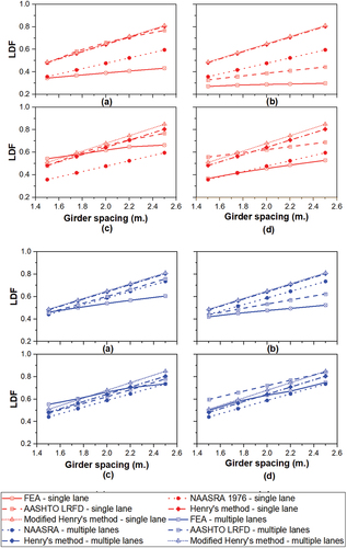
Figure 9(a, b) illustrate the moment LDFs of interior and exterior girders under single lane load, respectively, shown in red colour. Notably, the LDF derived from FEA for the interior girder exhibits the lowest value compared to other standards, as depicted in Figure 9(a). On the other hand, Figure 9(b) shows that AASHTO (2017) provides the smallest discrepancy and demonstrates a similar trend of interior moment LDF compared to the FEA results, with the highest and lowest LDFs occurring at the shortest and longest span lengths, respectively. However, it is noteworthy that the LDF of AASHTO (2017) closely resembles Henry’s and modified Henry’s methods, primarily due to the Lever rule method used to calculate the moment exterior girder LDF.

Moving on to two-lane bridges, Figure 9(a, b) present the moment LDFs in blue colour. As seen in Figure 9(b), the calculated moment interior LDF correlates well with AASHTO (2017), although AASHTO LRFD is slightly conservative, with the highest discrepancy at 5.25% when compared to LDFs from Australian bridges. Similarly, the exterior LDFs of Australian bridges exhibit a reasonable correlation with AASHTO (2017) and Henry’s and modified Henry’s methods.

Figure 9. LDF of I-girder (span length) with different LDF standards – red is single lane and blue is multiple lanes (a) bending moment – exterior girder (b) bending moment – interior girder (c) shear – exterior girder (d) shear – interior girder.

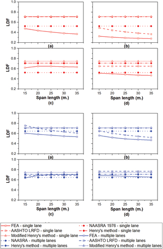
Figure 9(c, d) showcase the shear LDFs of interior and exterior girders in red. Similar to the moment LDFs, the shear LDFs from FEA also yield the lowest distribution factors. These shear LDFs from FEA, both for interior and exterior girders, exhibit a relatively constant value similar to AASHTO, Henry’s, and modified Henry’s methods. However, the LDFs from Australian I-girder bridges are generally lower when compared to the other standards.

Continuing with multiple traffic-lane situations for I-girder bridges, Figure 9(c, d) present the shear interior and exterior LDFs in blue. The shear interior girder LDFs also correlate well with AASHTO, Henry’s, and modified Henry’s methods. AASHTO LRFD again proves to be conservative compared to the LDFs from Australian bridges, while National Association of Australian State Road Authorities (1976) provides non-conservative LDFs. As depicted in Figure 9(c), the shear exterior LDFs under Australian geometries and T44 design load display a favourable relationship with AASHTO, Henry’s, and modified Henry’s methods. However, the modified Henry’s method estimates conservative LDF results when the span reaches 20 metres. Conversely, AASHTO LRFD and Henry’s method yield non-conservative LDFs when compared to the LDFs from Australian bridge models

7.2. I-girder bridges – girder spacing

Figure 10 depicts the LDF results of I-girder bridges with different girders spacing, ranging from 1.4 to 2.6 metres, as per the design norms in Australia. In Figure 10(a, b) (red), the bending moment of single lane load’s interior and exterior girders is showcased. The LDFs from other standard codes tend to produce conservative results within the girder spacing range for both interior and exterior girders when compared with LDFs from Australian bridges. Notably, National Association of Australian State Road Authorities (1976) yields the smallest discrepancy compared to LDF results in exterior girders, while AASHTO LRFD exhibits an excellent correlation with LDFs from Australian bridges. These observations are also consistent with the moment LDFs under multiple-lane load, as shown in blue in Figure 10(a, b).

Figure 10. LDF of I-girder (girder spacing) with different LDF standards – red is single lane and blue is multiple lanes (a) bending moment – exterior girder (b) bending moment – interior girder (c) shear – exterior girder (d) shear – interior girder.

Moving on to the comparison of shear LDFs (Figure 10(c, d)), the graphs illustrate results for both single and multiple lanes, represented in red and blue, respectively. The single-lane shear LDFs of Australian I-girder bridges exhibit a good correlation with AASHTO LRFD, whereas National Association of Australian State Road Authorities (1976) tends to provide non-conservative results under the critical load position. However, it is worth noting that National Association of Australian State Road Authorities (1976) shows an excellent correlation in the interior shear LDFs for multiple lanes.

7.3. I-girder bridges – girder depth

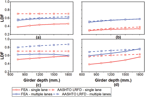
In accordance with AS 5100 (2017), an investigation was conducted on four I-girder standard sections with varying girder depths. The girder depth was altered following the I-girder standard sections in AS 5100 (2017), while maintaining a constant span length of 25 metres and a girder spacing of 2.2 metres. The LDFs for both interior and exterior girders, applicable to single and multiple-lane bridges, are presented in Figure 11(a–d).

Figure 11(a, b) display the bending moment for interior and exterior girders, respectively. The figures demonstrate that all other standard codes tend to produce conservative LDF results for both single and multiple-lane scenarios, whereas AASHTO LRFD exhibits a favourable correlation with LDFs obtained from Australian bridges.

Figure 11. LDF of I-girder (girder depth) with different LDF standards – red is single lane and blue is multiple lanes (a) bending moment – exterior girder (b) bending moment – interior girder (c) shear – exterior girder (d) shear – interior girder.

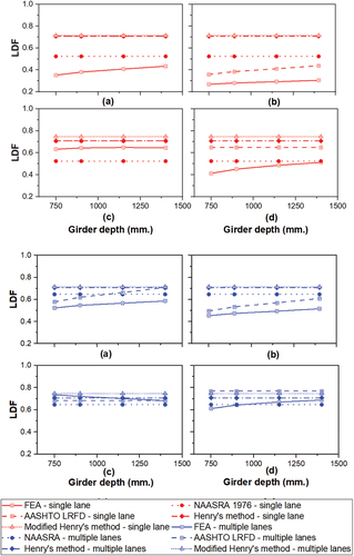
Moving on to Figure 11(c, d), which illustrate the shear LDFs for interior and exterior girders of the studied bridges, it becomes evident that all other standard codes also yield conservative LDF results compared to those of Australian I-girder interior girder bridges, except for National Association of Australian State Road Authorities (1976). For the shear LDF of exterior girders in single- and multiple-lane bridges, Australian bridges exhibit lower LDFs when compared to the other standard codes. These findings shed significant light on the performance and behaviour of I-girder bridges in Australia across a wide range of load scenarios and various parameters. They provide invaluable insights that can greatly contribute to optimising bridge design and enhancing safety considerations.

7.4. Super-T girder bridges – span length

The study focused on the LDFs of single-lane Super-T girder bridges, which were developed using FEA and then compared with AASHTO (2017) empirical equations, shown in red in Figure 12(a–d). Notably, National Association of Australian State Road Authorities (1976), Henry’s, and modified Henry’s methods were excluded from the comparison since they did not specify Super-T girder or similar geometries. However, to address this, the LDFs of open precast concrete boxes girder in AASHTO (2017) were selected as a comparative basis due to its similarity in geometry to the Super-T girder described in the standard.

Figure 12. LDF of Super-T bridges (span length) with different LDF standards – red is single lane and blue is multiple lanes (a) bending moment – exterior girder (b) bending moment – interior girder (c) shear – exterior girder (d) shear – interior girder.

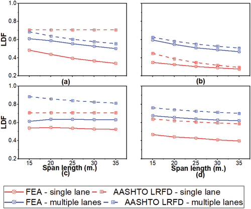
In Figure 12(a, b), the bending moment LDFs of two-lane Super-T girder bridges are represented by blue lines. It is evident from the figures that the LDFs from FEA and AASHTO (2017) exhibit a reasonable correlation, although with slight discrepancies. Similar to the single-traffic lane Super-T girder bridge (shown in red), the LDF is higher for shorter span lengths and lower for longer span lengths. For the moment interior girder, the calculated LDFs from AASHTO LRFD’s empirical equations slightly underestimate the results when compared with the LDFs of the Australian Super-T girder. Conversely, AASHTO LRFD provides a conservative estimation of moment exterior LDFs.

The bending LDFs of one-lane Super-T girder bridges for different span lengths are shown in Figure 12(a, b). Comparing the LDFs from FEA with the calculated LDFs from AASHTO (2017) reveals that the interior bending moment LDF is higher for the shortest span length of 15 metres and gradually decreases as the span length increases. The longest bridge span length in this study, 35 metres, has the lowest LDF for the interior bending moment. AASHTO LRFD and the Super-T girder derived from FEA exhibit a similar trend, but AASHTO LRFD estimates conservative LDFs at all spans. The exterior bending moment LDFs of one-lane Super-T girder bridges (shown in Figure 12(a)) also display a conservative trend for the shortest span length. Meanwhile, the exterior moment LDFs of AASHTO LRFD remain constant for different span lengths due to the application of the Lever rule, which provides conservative estimations of LDFs.

The shear LDF for single-lane Super-T girder bridges is presented in red in Figure 12(c, d), respectively. The LDFs of interior and exterior girders calculated from AASHTO (2017) provide conservative estimations at all span lengths, with significant discrepancies of 32% and 25.5% for interior and exterior shear, respectively.

Finally, Figure 12(c, d) in blue show the shear LDFs of multiple-lane Super-T girder bridges for different span lengths. The figures indicate that the LDFs between AASHTO LRFD and FEA have a reasonable correlation in terms of the trend. Nevertheless, AASHTO (2017) provides conservative results for interior and exterior shear LDFs, with maximum discrepancies of 2.5% and 33.47%, respectively.

7.5. Super-T girder bridges – girder spacing

The study considered the range of Super-T girder flanges to assess the girder spacing for Australian Super-T girder bridges. The girder spacing was increased while keeping the span length constant at 25 metres, using five girders of 750 mm Super-T girder depth. The moment and shear LFD results of Super-T girder bridges under varying girder spacing are displayed in Figure 13.

Figure 13. LDF of Super-T bridges (girder spacing) with different LDF standards – red is single lane and blue is multiple lanes (a) bending moment – exterior girder (b) bending moment – interior girder (c) shear – exterior girder (d) shear – interior girder.

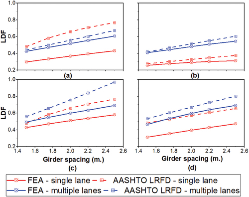
The figures reveal that AASHTO LRFD exhibits a strong correlation with Super-T girder bridges in terms of interior moment LDFs and interior and exterior shear LDFs. However, it is important to note that AASHTO LRFD tends to be highly conservative in estimating the exterior girder bending moment LDF, as it employs the Lever Rule for calculation. This conservatism is supported by previous studies conducted by Terzioglu et al. (2017), Yousif et al. (2007), and Puckett et al. (2011), which have shown that the Lever Rule consistently yields conservative results.

7.6. Super-T bridges – girder depth

In this study, the Super-T girder standard sections specified in AS 5100 (2017) were considered, encompassing five types of standard Super-T girder sections. The investigation involved increasing the depth of girders while maintaining a constant span length of 25 metres and a girder spacing of 2.2 metres. Figure 14 illustrates the results, indicating that the AASHTO LRFD LDF equations consistently yield conservative outcomes in both moment and shear for interior and exterior girders when compared with Super-T girder bridges, particularly under adverse longitudinal and transverse load directions.

Figure 14. LDF of Super-T bridges (girder depth) with different LDF standards – red is single lane and blue is multiple lanes (a) bending moment – exterior girder (b) bending moment – interior girder (c) shear – exterior girder (d) shear – interior girder.

Overall, the AASHTO LRFD LDF equations demonstrate a good correlation with the LDFs of both I-girder and Super-T girder bridges. However, it is essential to note that the application of the Lever Rule method in deriving LDFs for moment in the exterior girder of I-girder and Super-T girder bridges tends to result in a high level of conservativeness. This finding aligns with numerous studies that have also highlighted the Lever Rule method’s tendency to produce conservative results, thus confirming the observations made in this study.

These insights emphasise the significance of understanding and accounting for the conservativeness introduced by the Lever Rule method when designing I-girder and Super-T girder bridges. By considering this aspect in bridge design and analysis, engineers can ensure the appropriate level of safety and efficiency for these types of structures.

8. Conclusion and recommendation

In this research study, the primary focus was on deriving and contrasting Load Distribution Factors (LDFs) for Australian I-girder and Super-T girder bridges against various standard codes, thereby assessing their applicability within the Australian bridge context. The adoption of Finite Element Analysis (FEA) played an important role in computing the bridges’ load responses. This approach’s validity was established through comparisons with real-world field measurements and existing literature, culminating in the identification of an optimal mesh size. The T44 design load was chosen as a crucial parameter to derive LDFs, given its capacity to yield the most critical load positioning for both single and multiple-lane scenarios, resulting in the highest LDFs.

The research encompassed a wide range of typical I-girder and Super-T girder bridge geometries across a range of span lengths, girder spacings, and depths, aligning with Australian design criteria. This endeavour facilitated the determination of the most adverse LDFs inherent within the Australian bridge design space. Subsequently, the derived LDFs from Australian bridges were compared against empirically derived LDF equations from National Association of Australian State Road Authorities (1976), AASHTO (2017), Henry’s, and modified Henry’s methods.

The results of the comparison of LDFs led to the following conclusions:

• The comparison of LDFs derived from Australian I-girder bridges against various standard codes, including National Association of Australian State Road Authorities (1976), AASHTO (2017), Henry’s, and modified Henry’s methods, revealed predominantly conservative outcomes across different spans, girder spacings, and depths. Notably, AASHTO (2017) exhibited the highest degree of correlation with the other codes within this study.

• For Super-T girder bridges, a comparison was drawn between LDFs obtained via FEA and those from the open precast concrete box girder in AASHTO (2017). This examination demonstrated a consistent alignment, producing conservative results across various span lengths, girder depths, and spacings.

• The empirical equations stemming from AASHTO (2017) showcased commendable compatibility with both Super-T and I-girder bridges in the Australian context. While applicable for certain types of girders, load effects, and bridge spans, minor discrepancies emerged. Particularly, the Lever Rule method within AASHTO LRFD led to substantial conservatism when contrasted with LDFs of Australian bridges.

However, noteworthy distinctions emerged between LDFs derived from AASHTO (2017) empirical equations and those generated via FEA. These differences can be attributed to variations in standard cross-sectional configurations, especially when juxtaposed with Australian standard sections, resulting in distinct impacts on bridge girder stiffness. Furthermore, the influence of design loads as per AASHTO specifications and the selected vehicle load within this study, encompassing factors like axle spacing and total weight, significantly affected the load distribution along the bridge girder. These observations extended to the comparisons involving National Association of Australian State Road Authorities (1976), Henry’s, and modified Henry’s methods for I-girder bridges.

These disparities between FEA and various standard codes bear potential repercussions, potentially leading to overdesign and inaccurate bridge assessments. Consequently, the study advocates for the development of LDF equations tailored to typical Australian bridge geometries, aiming to enhance LDF accuracy during the design and evaluation phases.

The findings have highlighted the importance of employing appropriate empirical equations and FEA methodologies in bridge design, facilitating more accurate load distribution predictions for future projects. It is recommended that future studies should be on the development of LDF empirical equations for various types of Australian bridges, including Super-T, I-girder, and Box-girder bridges. The establishment of empirical equations will serve as a valuable resource for bridge engineers and asset managers, facilitating more effective preliminary bridge assessments and designs. By providing comprehensive LDF data specific to Australian bridge configurations, these empirical equations will enhance the accuracy and reliability of load distribution predictions, ultimately contributing to safer and more efficient bridge engineering practices.

9. Notations

Table

$A$	=	area of girder $(m{m}^2$)
$d$	=	depth of girder (mm)
$d_e$	=	distance from exterior web of exterior to the interior edge of curb (mm)
$E_B$	=	elastic modulus of beam material (MPa)
$E_D$	=	elastic modulus of deck material (MPa)
$e_g$	=	distance between the centres of gravity of the basic beam and deck (mm)
$I$	=	moment of inertia of beam $(m{m}^4)$
$K_g$	=	longitudinal stiffness parameter $(m{m}^4)$
$L$	=	span length of deck (mm)
$N_b$	=	number of girders
$S$	=	spacing of beams or webs (mm)
$t_s$	=	depth of concrete slab (mm)

Disclosure statement

No potential conflict of interest was reported by the author(s).

References

- AASHTO 2017. “AASHTO LRFD Bridge Design Specifications.”
- Ali, Afnan. 2018. “Incorporating Grillage Model Derived Load Distribution Factors into Ratings of Prestressed Concrete Bridges.”
- Barker, R. M., and J. A. Puckett. 1997. “Design of Highway Bridges Based on AASHTO LRFD Bridge Design Specifications.“ New York: John Wiley.
- Caprani, C. C., M. M. Melhem, and K. Siamphukdee. 2017. “Reliability Analysis of a Super-T Prestressed Concrete Girder at Serviceability Limit State to as 5100: 2017.” Australian Journal of Structural Engineering 18 (2): 60–72.
- Chen, Y., and A. Aswad. 1996. “‘Stretching Span Capability of Prestressed Concrete Bridges Under AASHTO LRFD.” Journal of Bridge Engineering 1 (3): 112–120. https://doi.org/10.1061/(ASCE)1084-0702(1996)1:3(112).
- DataVic 2021. “Bridge Structures.” https://discover.data.vic.gov.au/dataset/bridge-structures.
- Fatemi, S. J., A. H. Sheikh, and M. S. M. Ali. 2018. “Determination of Load Distribution Factors of Steel–Concrete Composite Box and I-Girder Bridges Using 3D Finite Element Analysis.” Australian Journal of Structural Engineering 19 (2): 131–145. https://doi.org/10.1080/13287982.2018.1452330.
- Hays, C. O., G. R. Consolazio, and M. I. Hoit. 1995. Metric/SI and PC Conversation of BRUFEM and SALOAD System. Report. Gainesville, FL, University of Florida.
- Hughs, E., and R. Idriss. 2006. “Live-Load Distribution Factors for Prestressed Concrete, Spread Box-Girder Bridge.” Journal of Bridge Engineering 11 (5): 573–581. https://doi.org/10.1061/(ASCE)1084-0702(2006)11:5(573).
- Huo, X. S., S. O. Conner, and R. Iqbal. 2003. “Re-Examination of the Simplified Method (Henry’s Method) of Distribution Factors for Live Load Moment and shear.“ TNSPR-RES 1218.
- Kim, Y. J., and Y. Ji. 2019. “Evaluation of Prestressed Concrete Bridges Under Light Rail Loading.” American Concrete Institute Structural Journal 116 (1): 171–182. https://doi.org/10.14359/51706921.
- Melhem, M., C. Caprani, M. G. Stewart, and S. Zhang. 2020. Bridge Assessment Beyond the as 5100 Deterministic Methodology. Austroads, Sydney NSW Australia. https://austroads.com.au/publications/bridges/ap-r617-20>.