Characteristics of earthquake ground motions requiring extended dynamic analysis

ABSTRACT

The absolute maximum response (AMR) of structures might occur posterior to the end of earthquake excitations, hence, extending the dynamic analysis to the post-shaking phase is required. This phenomenon was found to be more common for long-period and low-damping structures, which are prevailing in regions of low-to-moderate seismicity like Australia. In this article, the mechanism of the occurrence of AMR in the post-shaking phase is first explained using single-degree-of-freedom (SDOF) systems subjected to a simple sine wave. Further investigation on real earthquake ground motions reveals that whether an extended analysis is required depends greatly on the characteristics of the post-significant duration phase. Finally, suitable metrics for describing ground motions that require extended analysis (EAGMs) are identified based on the Kolmogorov–Smirnov test. Regression analyses are then conducted to predict the probability of EAGMs.

KEYWORDS:

• Earthquake
• response spectrum
• dynamic analysis
• post-significant duration
• Kolmogorov–Smirnov test

1. Introduction

A recent study conducted by the authors (Yi and Tsang 2023) has revealed for the first time an important phenomenon of real earthquake ground motions, to which the maximum structural response might occur posterior to the end of the ground shaking. In other words, the peak response calculated within the during-shaking phase might significantly underestimate the actual structural demands. If the underestimation occurs for any structural periods between 0 and 20 s, the ground motion would require an extended analysis and is regarded as an EAGM.

The ground motions randomly selected from the PEER NGA-West2 database (Ancheta et al. 2014) for this study, including 255 non-pulse-like three-component records and 139 pulse-like ones, are listed in Appendix A and the identified EAGMs based on acceleration response are listed in Appendix B. The percentages of non-pulse-like EAGMs identified under a 5% damping ratio and the pulse-like EAGMs under a 2% damping ratio are 3.8% and 3.6%, respectively. To accurately capture the absolute maximum response (AMR), it is recommended that dynamic analysis should be extended by half of the structural period after the excitation ends.

To perform earthquake-resistant design in accordance with seismic codes and standards, dynamic analyses are performed based on a few input ground motions only. For instance, a set of at least three ground motion records is required for response history analyses as stipulated in the Eurocode 8 (CEN 2004), Australian Standard AS1170.4 (Standards Australia 2007) and New Zealand Standard NZS1170.5 (Standards New Zealand 2004). The same number of ground motion pairs is required by ASCE/SEI 7 for linear analyses, whereas a minimum of seven pairs is required for nonlinear analyses (ASCE/SEI 2007). If some of those selected ground motions are EAGMs, this could lead to an underestimation of the structural demand and in turn reduce the safety level of the structure.

EAGMs are more likely to develop for low-damping and/or long-period structures (Yi and Tsang 2023) including high-rise buildings (Bernal et al. 2015; Cruz and Miranda 2017), long-span bridges such as suspension bridges and cable-stayed bridges (Gimsing and Georgakis 2012; Li et al. 2018), and low-ductility structures such as unreinforced masonry structures (Elmenshawi et al. 2010), which are typically constructed in regions of low-to-moderate-seismicity including Australia. For example, high-rise buildings with heights exceeding 45 m have damping ratios of 3% or lower (PEER 2017). The taller the building is, the longer the fundamental natural period and the lower the damping ratio generally. Moreover, many of these long-period structures are critical infrastructures or categorised into higher importance classes. The consequences of damage or collapse of these structures would be unbearable. This highlights the significance of identifying EAGMs in seismic design. Hence, this study intends to develop a better understanding of EAGMs by explaining the mechanism and investigating their characteristics.

First, the post-shaking response of SDOF systems under a simple sine wave is illustrated and the mechanism of the occurrence of AMR posterior to the shaking is explained, with a particular focus on the effects of the structural period and damping level. Then, the characteristics of the identified EAGMs are investigated and the effect of the post-significant duration is highlighted. Finally, suitable metrics for describing EAGMs are identified and regression analyses are then conducted to provide a tool for predicting the probability of EAGMs and the range of structural periods that requires extended analysis based on these metrics.

2. Post-shaking response under a sine wave

2.1. During-shaking response and post-shaking response

The governing equation of motions ($u$, $\dot{u}$, $\ddot{u}$) of a linear single-degree-of-freedom (SDOF) system subjected to ground acceleration $\underset{g}{\ddot{u}}(t)$ is expressed as:

(1) $\ddot{u}\left(t\right)+2\xi w\dot{u}\left(t\right)+w^{2}u\left(t\right)=-\underset{g}{\ddot{u}}\left(t\right)$(1)

where $\omega$ and $\xi$ are the circular frequency and the damping ratio of the SDOF system, respectively. Taking a single cycle of a sine wave with a period of 1 s expressed in Equation (2)(2) $\underset{g}{\ddot{u}}\left(t\right)=\sin \left(2\pi t\right)\left(0\le t\le 1s\right)$(2) for illustration, Figure 1 shows the response history of a SDOF system with a natural period (T_n = 2π/$\omega$) of 3 s and a damping ratio of 5%.

(2) $\underset{g}{\ddot{u}}\left(t\right)=\sin \left(2\pi t\right)\left(0\le t\le 1s\right)$(2)

Figure 1. (a) a single cycle of an input sine-wave acceleration with a period of 1 s, and the (b) acceleration response, (c) velocity response, and (d) displacement response time series of a SDOF system (T_n = 3 s, $\xi =5\%$).

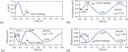
Figure 1 shows that the system develops dynamic responses both during and after the shaking. Thus, the structural responses can be divided into two phases, the during-shaking phase (0 ≤ t ≤ t_max, where t_max is the duration of the excitation and in this case t_max = 1 s) and the post-shaking phase (t > t_max). In the during-shaking phase, the system develops forced vibration, whereas it develops free vibration in the post-shaking phase.

In the during-shaking phase, ‘phase lag’ between the structural responses and the input ground motions can clearly be observed. The first peak of the input ground acceleration occurs at 0.25 s, whereas the first peaks of the acceleration, velocity and displacement responses of the system occur at 0.69 s, 0.45 s and 0.74 s, respectively. This is because the system has zero displacement and velocity at the onset of the excitation, and it takes time for the structure to develop the first peak response. Figure 1 shows that the system has not completed a full cycle of response at the end of the shaking, as the natural period of the system is 3 s, while the input ground motion lasts for 1 s only. Hence, the second peaks of the responses likely occur after the input motion ends.

In the post-shaking phase, the system vibrates freely depending on the motions at the end of the shaking (t = t_max). For the system with 5% damping, the second (negative) peak acceleration response is 16% larger than the first (positive) peak. Meanwhile, the positive acceleration response at t = t_max (Figure 1b) leads to a continuous increase in the velocity response until the acceleration response becomes negative (Figure 1c), at which, the velocity response attains its maximum that is 9% higher than the first peak in the during-shaking phase. Likewise, the relatively long period of positive velocity response leads to a long period of displacement response from a smaller negative value at the end of the shaking to a larger positive value that is 17% higher (Figure 1d). The responses of the second peaks are larger than the first peaks likely because it takes time for resonance to develop. The resonant response would have a larger amplitude, which is not suppressed if the damping level is not high enough. The phenomenon described above indicates that the natural period and the damping level play important roles in the post-shaking response. They will be investigated further in the rest of this article.

For seismic design, it is vital to accurately capture the absolute maximum response. This illustration based on a simple sine wave depicted in Figure 1 clearly shows that the SDOF system would develop AMRs during the post-shaking phase. If the response history analysis is conducted only in the during-shaking phase, the real AMR of the SDOF system might be underestimated. For the sake of further investigation, such underestimation is quantified in this study by:

(3) $\beta =\frac{\mathrm{A}\mathrm{M}{\mathrm{R}}_{\mathrm{d}\mathrm{u}\mathrm{r}}}{\mathrm{A}\mathrm{M}\mathrm{R}}\le 1$(3)

where $\mathrm{A}\mathrm{M}{\mathrm{R}}_{\mathrm{d}\mathrm{u}\mathrm{r}}$ is the absolute maximum response in the during-shaking phase (indicating that only the during-shaking response is considered) and $\mathrm{A}\mathrm{M}\mathrm{R}$ is the actual absolute maximum response considering both the during-shaking phase and the post-shaking phase. In Figure 1, the values of $\beta$ are 0.853, 0.927 and 0.850 for acceleration, velocity and displacement, respectively.

In the post-shaking phase, due to the damping effect, the peak response at each half cycle would be gradually reduced. Thus, the AMR in the post-shaking phase must be reached within the first half cycle of the free vibration (Chopra 2023). Therefore, it was recommended by Yi and Tsang (2023) that a dynamic analysis should be extended to half of the structural period of the SDOF system if the maximum response is of interest. This is also illustrated in Figure 1, where the times of the AMR (denoted by t_AMR hereafter) for acceleration, velocity and displacement response are all smaller than 1 s + 1.5 s = 2.5 s in which 1 s is the duration of the sine wave and 1.5 s is half of the structural period of the SDOF system.

2.2. Response spectra of a single sine wave

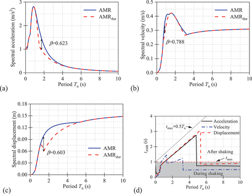
The calculation in the previous subsection is repeated for a series of SDOF systems with different natural periods. Figure 2 shows the actual response spectra (denoted by AMR in the legend) with a 5% damping ratio and the corresponding t_AMR under the simple sine-wave motion as expressed in Equation (2)(2) $\underset{g}{\ddot{u}}\left(t\right)=\sin \left(2\pi t\right)\left(0\le t\le 1s\right)$(2) . The traditional approach for calculating the response spectrum based on the AMR_dur is also superimposed on the figure for direct comparison. It is illustrated that structural periods play an important role in determining whether the AMR develops in the during-shaking phase or the post-shaking phase. The period window in which the AMR occurs in the post-shaking phase (t_AMR > t_max, t_max = 1 s) would be T_n = 1–4.8 s and T_n = 1–5.3 s for the acceleration and displacement response spectrum, respectively, while it is T_n = 0.65–1.3 s and T_n = 2.2–3.2 s for the velocity response spectrum. Within these period ranges, t_AMR increases in an almost linear fashion with the structural period, while t_AMR suddenly drops below 1 s when the structural period exceeds a certain value. Figure 2(d) indicates that t_AMR is generally smaller than t_max +0.5T_n as a result of the damping effect in the post-shaking phase. Figure 2 also shows that the value of $\beta$ varies significantly with the structural periods. The range of $\beta$ would be 0.623–1.0, 0.788–1.0 and 0.603–1.0 for acceleration, velocity and displacement response, respectively.

Figure 2. Response spectra and t_AMR of $\stackrel{\hspace{0.17em}}{\underset{g}{\overset{\hspace{0.17em}}{u}}}(t)=sin\left(2\pi t\right)\left(0\le t\le 1\mathrm{s}\right)$ under 5% damping ratio: (a) spectral acceleration, (b) spectral velocity, (c) spectral displacement and (d) the time of the AMR, t_AMR.

2.3. Effect of damping

The investigation above focuses on a fixed damping ratio of 5%, whereas the responses of a SDOF system can be significantly affected by the level of damping. Figure 3 shows the response histories of an SDOF system (T_n = 3 s) with different damping ratios subjected to the simple sinusoidal motion of Equation (2)(2) $\underset{g}{\ddot{u}}\left(t\right)=\sin \left(2\pi t\right)\left(0\le t\le 1s\right)$(2) . Table 1 lists the maximum responses of the SDOF system in the during-shaking phase (AMR_dur) and post-shaking phase (AMR_post) as well as the resulting values of $\beta$. Figure 3 and Table 1 illustrate that in the during-shaking phase, the time histories might be slightly affected by the damping ratio, while AMR_dur is not significantly affected. The reason is that the input motion is of relatively short duration, compared to the period of the structure, such that the peak response is reached within a short time before the energy in the structure is dissipated through damping. On the contrary, during the post-shaking phase, both time histories and peak responses are significantly affected by the damping ratio, and the peak response is reached earlier and reduced significantly with the increase in the damping ratio. As a result, the values of $\beta$ increase with the damping ratios. When the damping ratio increases to 20%, the occurrence of the AMR shifts from the post-shaking phase to the during-shaking phase. This finding reconciles with the suppressive effect of damping on resonant response. Whether AMR occurs in the during-shaking phase or the post-shaking phase depends on the counteraction between the resonant effect and the damping effect.

Figure 3. Effect of damping on response histories of a SDOF system (T_n = 3.0 s) under the sine wave $\stackrel{\hspace{0.17em}}{\underset{g}{\overset{\hspace{0.17em}}{u}}}(t)=sin\left(2\pi t\right)\left(0\le t\le 1\mathrm{s}\right)$.

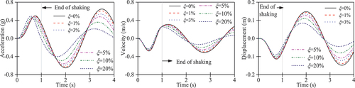
Table 1. Absolute maximum response (AMR) and underestimation ratio $\beta$ of a SDOF system (T_n  = 3.0 s) under the sine wave $\stackrel{\hspace{0.17em}}{\underset{g}{\overset{\hspace{0.17em}}{u}}}(t)=sin\left(2\pi t\right)\left(0\le t\le 1\mathrm{s}\right)$

Damping ratio	Acceleration			Velocity			Displacement
	AMRdur (g)	AMRpost (g)	$\beta$	AMRdur (m/s)	AMRpost (m/s)	$\beta$	AMRdur (m)	AMRpost (m)	$\beta$
$\xi =0\mathrm{\%}$	0.500	0.649	0.77	0.276	0.310	0.89	0.114	0.148	0.77
$\xi =1\mathrm{\%}$	0.494	0.630	0.79	0.273	0.305	0.89	0.113	0.144	0.78
$\xi =3\mathrm{\%}$	0.486	0.593	0.82	0.268	0.297	0.91	0.110	0.135	0.82
$\xi =5\mathrm{\%}$	0.479	0.561	0.85	0.266	0.289	0.92	0.108	0.127	0.85
$\xi =10\mathrm{\%}$	0.474	0.493	0.96	0.264	0.273	0.97	0.102	0.110	0.92
$\xi =20\mathrm{\%}$	0.490	0.403	1.00	0.254	0.254	1.00	0.092	0.085	1.00

For the same input motion, the response spectra are calculated for different damping ratios, and the values of $\beta$ for acceleration, velocity and displacement response are also calculated, as shown in Figure 4(a–c). Figure 4(d) shows the t_AMR for the acceleration spectrum. Figure 4 shows that both $\beta$ and t_AMR values are significantly affected by the damping ratio. In general, the lower threshold value of the period window for the AMR occurring in the post-shaking phase remains unchanged, which is 1 s for acceleration and displacement response spectra and 0.65 s for the velocity response spectra. It is noted that the lower threshold value for acceleration and displacement spectra is exactly the period of the sine wave. This indicates that EAGMs for acceleration and displacement response occur only when the structural period is larger than the period of the sine wave. Therefore, EAGMs would be more likely to occur for long-period structures.

Figure 4. Effect of damping on underestimation ratio $\beta$: (a) spectral acceleration, (b) spectral velocity, (c) spectral displacement and (d) effect of damping on t_AMR for acceleration spectra under the sine wave $\stackrel{\hspace{0.17em}}{\underset{g}{\overset{\hspace{0.17em}}{u}}}(t)=sin\left(2\pi t\right)\left(0\le t\le 1\mathrm{s}\right)$.

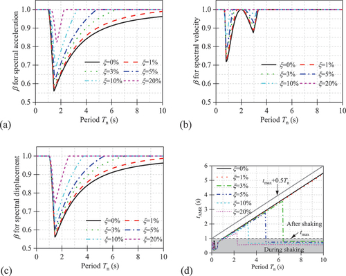
On the other hand, the upper threshold value of the period window for the AMR occurring in the post-shaking phase tends to decrease with the increase of damping ratios. This is because, with smaller damping, SDOF systems of long structural periods require longer times to reach AMR, as reflected by the large values of t_AMR in Figure 4(d). As the damping increases, the energy is dissipated more rapidly, and it reduces AMR_post in the post-shaking phase. Meanwhile, the value of $\beta$ increases with the damping ratio during these period windows. The results above indicate that damping to some extent inhibits the development of the AMR in the post-shaking phase. However, it is noted that even for $\xi =20\mathrm{\%}$, there still exists a period window for the AMR to be developed in the post-shaking phase.

Another observation drawn from Figure 4 is that acceleration and displacement spectra share similar variations of the values of $\beta$ against the periods, whereas the velocity spectrum exhibits a very different pattern. For a given damping ratio, both acceleration and displacement spectra have wider period windows with t_AMR > t_max, than the velocity spectrum. Meanwhile, t_AMR is less than t_max +0.5T_n for all the cases. This indicates that calculating the response spectra of sinusoidal input motions should be extended to the post-shaking phase by half of the structural periods, especially for acceleration and displacement spectra.

3. Importance of post-significant duration

The result based on a sine wave indicates that the occurrence of AMR in the post-shaking phase occurs for systems with longer natural periods, whereas the damping has a suppressive effect on the development of the post-shaking response. Real ground motions can be regarded as complex motions that contain a random combination of simple sinusoidal waves of different frequencies originating from successive ruptures occurring at different locations and times. The recording of the ground motions is triggered when shaking occurs and ceased when the ground shaking falls under an imperceptible level. As a result, real earthquake ground motions usually have a much longer duration than the sine wave presented in Section 2 and have relatively low amplitudes in the tail part of the shaking. Due to the damping effect, the characteristics of the tail part would play an important role in an EAGM.

3.1. Post-significant duration of ground motions

The duration of a ground motion record is an important parameter that has an important effect on structural performance. A number of metrics have been widely used to quantify ground motion duration, including bracketed duration, uniform duration and significant duration (Bommer and Martínez-Pereira 1999; Fayaz, Medalla, and Zareian 2020; Hou and Qu 2015; Kiani, Camp, and Pezeshk 2017). The first two metrics are determined based on absolute predefined values, whereas the last one depends on the relative distribution of the time series. In this study, the concept of significant duration is adopted. There are two common methods to define significant duration. The first one makes use of a well-known integration-based accumulative intensity measure, Arias Intensity (AI) (Arias 1970), as expressed in Equation (4)(4) $\mathrm{A}\mathrm{I}=\frac{\pi }{2g}{\int }_0^{t_{\mathrm{m}\mathrm{a}\mathrm{x}}}{a}^2\left(t\right)dt$(4) . The significant duration is defined as the time interval between certain amounts of total energy, such that a specific percentage of AI is accumulated.

(4) $\mathrm{A}\mathrm{I}=\frac{\pi }{2g}{\int }_0^{t_{\mathrm{m}\mathrm{a}\mathrm{x}}}{a}^2\left(t\right)dt$(4)

where $t_{\mathrm{m}\mathrm{a}\mathrm{x}}$ is the total duration of the record, such that AI is calculated for the entire duration of the shaking. Alternatively, cumulative absolute velocity (CAV) (Reed and Kassawara 1990), expressed in Equation (5)(5) $\mathrm{C}\mathrm{A}\mathrm{V}={\int }_0^{t_{\mathrm{m}\mathrm{a}\mathrm{x}}}\left|a\left(t\right)\right|dt$(5) , can be used to assess the effect of ground motion duration on structural responses.

(5) $\mathrm{C}\mathrm{A}\mathrm{V}={\int }_0^{t_{\mathrm{m}\mathrm{a}\mathrm{x}}}\left|a\left(t\right)\right|dt$(5)

In the present study, t_x denotes the time when the specified percentage (x%) of normalised AI or CAV is attained. t_AIx-y is defined as the time interval between a minimum x% and a maximum y% of the normalised AI. Normally, t_AI5–95 is used to define the significant duration of a ground motion and t_AI95–100 for the post-significant duration. Similarly, t_CAV5–95 and t_CAV95–100 are employed to represent the time intervals of significant duration and post-significant duration with respect to CAV.

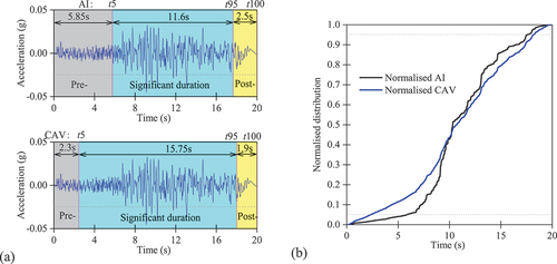
Figure 5 shows an example of the significant duration based on the normalised AI and CAV of the H2 component of RSN94. The pre-, during- and post-significant duration phases are shaded in grey, cyan and yellow, respectively. RSN94 has a rupture distance of 62.23 km. This motion is selected for illustration as it is identified as a typical EAGM.

Figure 5. Significant duration of H2 component of RSN94: (a) three phases of the acceleration time series based on AI (top) and CAV (bottom) and (b) normalised AI and CAV against time..

3.2. Effect of post-significant duration

Figure 6 shows the sample response time series of SDOF systems ($\xi$ = 5%) with a natural period of T_n = 1.5 s, 3.5 s and 7.8 s under the H2 component of RSN94. Note that the stated significant duration is calculated based on their CAV5–95. In Figure 6 that investigates the effect of post-significant duration, two cases are considered: Case 1, which ignores the ground shaking in the post-significant duration phase by setting the acceleration values to zero; and Case 2, which considers the full ground motion record.

Figure 6. Response histories of three SDOF systems ($\xi =5\%$) under H2 component of RSN94 without (Case 1) and with (Case 2) post-significant duration phase.

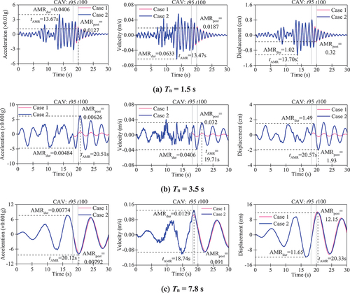
Figure 6(a) illustrates that, for T_n = 1.5 s, the input ground acceleration in the post-significant duration phase would slightly alter the response histories after t₉₅, but the AMR would not be affected, as AMR occurs within the significant duration phase. Figure 6(b) shows that, for T_n = 3.5 s, the acceleration, velocity and displacement response histories in Case 1 would reach the maximum values during the significant duration phase while the response would become very low in the post-significant duration phase. On the other hand, very large responses are induced in Case 2, and AMRs of acceleration and displacement occur posterior to the end of the shaking. This indicates that it is the post-significant duration phase, rather than the significant duration phase, that is responsible for the AMR. Figure 6(c) shows that, for T_n = 7.8 s, the response histories are not significantly different between the two cases, and the AMRs of acceleration and displacement develop posterior to the significant duration phase. This indicates that the AMR is mainly attributed to the significant duration and the length of the post-significant duration is too short to develop larger acceleration and displacement responses.

The discussion above indicates that EAGMs might be mainly induced by two mechanisms. In Mechanism 1, the post-significant duration is responsible for the AMR, which occurs posterior to the post-significant duration phase. This indicates that the relative contribution of the post-significant duration phase to the AMR is significant. In Mechanism 2, significant duration phase is responsible for the AMR, but the post-significant duration phase is too short for the development of AMR, depending on the structural periods.

4. Metrics for describing EAGMs

The discussion in the previous section shows that the length of the post-significant duration phase and its relative contribution to the structural responses in combination play an important role in determining whether a ground motion belongs to EAGMs. This section attempts to determine the appropriate metrics for describing EAGMs. Since acceleration spectra are more commonly used than the other two, only acceleration spectra are discussed hereafter.

The following eight metrics are taken into consideration: (1) PGA: peak ground acceleration, adopted for its wide application in characterizing the intensity of a ground motion; (2) t_max: the maximum duration of the ground motion; (3) t_AI95–100: the time interval between 95% and 100% of the normalised AI; and (4) t_CAV95–100: the time interval between 95% and 100% of the normalised CAV. Both t_AI95–100 and t_CAV95–100 are measurements for the length of the post-significant duration phase, thus mainly taking into account Mechanism 2 of EAGMs.

Moreover, to consider Mechanism 1, the relative ground acceleration intensity between the significant duration phase and the post-significant duration phase is calculated based on the concept of mean-square acceleration (Kolli and Bora 2021; McCann and Shah 1979) as defined by:

(6) $a_{\mathrm{m}\mathrm{s}}^2\left(t_2,t_1\right)=\frac{{\int }_{t_1}^{t_2}{a}^2\left(t\right)dt}{t_2-t_1}$(6)

Therefore, the ratio of mean-square acceleration between the significant duration phase and the post-significant duration phase can be expressed as:

(7) $\left(5\right)R_{\mathrm{a}\mathrm{A}\mathrm{I}95-100}=\frac{a_{\mathrm{m}\mathrm{s}}^2\left(\mathrm{t}5,\hspace{0.17em}t95\right)}{a_{\mathrm{m}\mathrm{s}}^2\left(\mathrm{t}95,\hspace{0.17em}t100\right)}=\frac{\frac{{\int }_{t5}^{t95}{a}^2\left(t\right)dt}{t95-t5}}{\frac{{\int }_{t95}^{t100}{a}^2\left(t\right)dt}{t100-t95}}=\frac{2\times 90\mathrm{\%}\times AI\cdot g/\left(\pi \cdot t_{\mathrm{A}\mathrm{I}5-95}\right)}{2\times 5\mathrm{\%}\times AI\cdot g/\left(\pi \cdot t_{\mathrm{A}\mathrm{I}95-100}\right)}=18\frac{t_{\mathrm{A}\mathrm{I}95-100}}{t_{\mathrm{A}\mathrm{I}5-95}}$(7)

Similarly, $R_{\mathrm{a}\mathrm{C}\mathrm{A}\mathrm{V}95-100}$, with respect to the ratio of absolute acceleration, is expressed as:

(8) $(6)R_{\mathrm{a}\mathrm{C}\mathrm{A}\mathrm{V}95-100}=18\frac{t_{\mathrm{C}\mathrm{A}\mathrm{V}95-100}}{t_{\mathrm{C}\mathrm{A}\mathrm{V}5-95}}$(8)

Both $R_{\mathrm{a}\mathrm{A}\mathrm{I}95-100}$ and $R_{\mathrm{a}\mathrm{C}\mathrm{A}\mathrm{V}95-100}$, associated with ground acceleration intensity, are used to mainly take into account Mechanism 1. In addition, the following two metrics are defined to consider both Mechanism 1 and Mechanism 2 by combining the length of the post-significant duration phase and the relative ground acceleration intensity:

(9) $\left(7\right)R{T}_{\mathrm{A}\mathrm{I}95-100}=\frac{t_{\mathrm{A}\mathrm{I}95-100}}{t_{\mathrm{A}\mathrm{I}5-95}}{t}_{\mathrm{A}\mathrm{I}95-100}$(9)

(10) $\left(8\right)R{T}_{\mathrm{C}\mathrm{A}\mathrm{V}95-100}=\frac{t_{\mathrm{C}\mathrm{A}\mathrm{V}95-100}}{t_{\mathrm{C}\mathrm{A}\mathrm{V}5-95}}{t}_{\mathrm{C}\mathrm{A}\mathrm{V}95-100}$(10)

RT_AI95–100 can be considered as the product of t_AI95–100 and $R_{\mathrm{a}\mathrm{A}\mathrm{I}95-100}$ divided by 18, whereas RT_CAV95–100 is the product of t_CAV95–100 and $R_{\mathrm{a}\mathrm{C}\mathrm{A}\mathrm{V}95-100}$ divided by 18.

The real earthquake ground motions employed in Yi and Tsang (2023) are listed in Appendix A. Figures 7–8 show the distributions of EAGMs and non-EAGMs for non-pulse-like and pulse-like ground motions in terms of different metrics under a 1% damping ratio. They clearly demonstrate that the distribution of EAGMs and non-EAGMs varies with the metrics, and selecting the proper metrics can help distinguish between EAGMs and non-EAGMs. To this end, the Kolmogorov – Smirnov test (Lilliefors 1967) is adopted. It is a non-parametric statistical method for comparing two empirical distributions, and it defines the largest absolute difference between the two cumulative distribution functions as a measure of disagreement (Lopes, Hobson, and Reid 2008; Song et al. 2005). The EAGMs and non-EAGMs are separately sorted by each metric and the cumulative distribution function is derived. For instance, suppose that the random samples of EAGMs of size m are endowed with statistical order as X₍₁₎, X₍₂₎, … , X_(m), the cumulative distribution function is determined as:

Figure 7. Distribution of EAGMs and non-EAGMs based on eight metrics for describing non-pulse-like ground motions ($\xi$ = 1%).

Figure 8. Distribution of EAGMs and non-EAGMs based on eight metrics for describing pulse-like ground motions ($\xi$ = 1%).

(11) $F\left(x\right)=\{\begin{array}{cc}0& \mathrm{i}\mathrm{f}x<X_{\left(1\right)}\\ k/m& \mathrm{i}\mathrm{f}{X}_{\left(k\right)}\le x\le X_{\left(k+1\right)}\\ 1& \mathrm{i}\mathrm{f}x\ge X_{\left(m\right)}\end{array}$(11)

The null hypothesis is that the samples of EAGMs and non-EAGMs belong to the same distribution functions with respect to a given metric. The p-value(s) of the Kolmogorov–Smirnov test is the probability of observing the test as more extreme than the observed value under the null hypothesis. The validation of the null hypothesis is questioned for small p-value(s), like those smaller than 0.05. The smaller the p-value(s), the larger the difference between EAGMs and non-EAGMs, and the easier it is to isolate EAGMs from non-EAGMs. As the Kolmogorov – Smirnov test is conducted with different metrics, the most suitable metrics for distinguishing between EAGMs and non-EAGMs can then be identified with the lowest p-value(s).

Table 2 reveals that PGA, with p-values larger than 0.05 in some cases under non-pulse-like ground motions and all cases under pulse-like ones, would not be a good metric for distinguishing between EAGMs and non-EAGMs. The p-values of t_max are smaller than those of PGA for most cases, but not as small as for other metrics. For non-pulse-like ground motions, t_AI95–100, t_CAV95–100, $R_{\mathrm{a}\mathrm{A}\mathrm{I}95-100}$ and $R_{\mathrm{a}\mathrm{C}\mathrm{A}\mathrm{V}95-100}$ are identified as good metrics for distinguishing EAGMs from non-EAGMs. This indicates that in non-pulse-like ground motions, Mechanism 1 and Mechanism 2 widely exist in EAGMs. As a consequence, RT_AI95–100, by taking into account both mechanisms, is a better indicator than t_AI95–100 and $R_{\mathrm{a}\mathrm{A}\mathrm{I}95-100}$. Similarly, RT_CAV95–100 surpasses t_CAV95–100 and $R_{\mathrm{a}\mathrm{C}\mathrm{A}\mathrm{V}95-100}$. Meanwhile, Table 2 also reveals that t_CAV95–100 is a better indicator than t_AI95–100, $R_{\mathrm{a}\mathrm{C}\mathrm{A}\mathrm{V}95-100}$ is better than $R_{\mathrm{a}\mathrm{A}\mathrm{I}95-100}$, and RT_CAV95–100 is better than RT_AI95–100. The discussion above indicates that RT_CAV95–100 is most suitable for characterising non-pulse-like EAGMs.

Table 2. P-value(s) of Kolmogorov–Smirnov test on eight metrics for describing EAGMs and non-EAGMs.

Damping ratio	PGA	tmax	tAI95–100	tCAV95–100	$R_{\mathrm{a}\mathrm{A}\mathrm{I}95-100}$	$R_{\mathrm{a}\mathrm{C}\mathrm{A}\mathrm{V}95-100}$	RTAI95–100	RTCAV95–100
Non-pulse-like ground motions
1%	.0022	2.71E–24	3.95E–21	1.25E–28	2.43E–14	7.92E–20	1.21E–17	7.08E–26
2%	.0003	1.75E–16	1.87E–19	1.29E–24	1.17E–14	1.48E–21	4.20E–20	1.90E–28
3%	1.92E–05	2.87E–12	8.73E–18	3.81E–25	3.31E–13	7.94E–20	4.70E–18	1.50E–26
5%	.0166	2.64E–07	1.06E–14	2.50E–14	8.26E–10	4.04E–11	3.07E–14	1.38E–15
7%	.0385	0.0011	6.47E–10	2.09E–08	1.69E–06	9.94E–08	1.22E–08	8.13E–09
10%	.0688	0.0830	0.0001	0.0005	0.0001	0.0002	5.03E–05	0.0003
15%	.3437	0.0321	0.0251	0.0254	0.0325	0.0205	0.0271	0.0208
Pulse-like ground motions
1%	.6462	4.20E–07	8.10E–06	2.85E–08	0.0602	0.0002	0.0010	1.51E–07
2%	.3091	2.72E–06	2.77E–05	2.34E–05	0.0779	0.0173	0.0008	0.0002
3%	.5717	0.0002	0.0009	0.0006	0.1173	0.0363	0.0125	0.0021
5%	.9281	0.0921	0.0255	0.0232	0.0184	0.0128	0.0184	0.0145
7%	.9281	0.0921	0.0255	0.0232	0.0184	0.0128	0.0184	0.0145

For pulse-like ground motions, t_AI95–100 and t_CAV95–100 are found with the smallest p-values while the p-values for $R_{\mathrm{a}\mathrm{A}\mathrm{I}95-100}$, $R_{\mathrm{a}\mathrm{C}\mathrm{A}\mathrm{V}95-100}$, RT_AI95–100 and RT_CAV95–100 are generally much larger. This indicates that the main cause of pulse-like EAGMs is generally the short length of the post-significant duration phase (Mechanism 2). This is a reasonable outcome because, in pulse-like ground motions, most of the seismic energy is contained in the velocity pulses that typically appear within the significant duration phase. Thus, it is unlikely that the ground shaking in the post-significant duration phase would cause the maximum response. Due to the impulsive nature of velocity pulses, there would be a considerable chance that the AMR occurs posterior to the shaking if the post-significant duration is too short. Compared to t_AI95–100, t_CAV95–100, which has smaller p-values, is identified as the best metrics to describe pulse-like EAGMs.

5. Prediction of EAGM

5.1. Probability of EAGMs

This study is based on a subset of recorded ground motions obtained from the PEER NGA-West2 database, and the information of some EAGMs is shown in Appendix B. It is desirable to investigate all available ground motions individually so that all EAGMs are identified; however, this might require a substantial amount of work. Meanwhile, new ground motions are being recorded worldwide, and much work is needed to categorise them into EAGMs and non-EAGMs. Besides real ground motions, the response spectra of some other excitations are widely used for structural assessment, such as floor response spectra (Shang, Li, and Wang 2022) and the response spectra of mine blast-induced ground vibrations (Tsang et al. 2018) and synthetic earthquake ground motions (Tang, Lam, and Tsang 2021). Before calculating the response spectra of these excitations, knowing if an extended analysis is required would be helpful. In this respect, regression analysis is performed on the probability of EAGMs based on the most suitable metrics as identified in the previous subsection.

The method is described as follows. First, the ground motions are sorted using the appropriate metrics from low to high values. The non-pulse-like ground motions are sorted by RT_CAV95–100 and pulse-like ground motions by t_CAV95–100. Then, the ground motions are compiled into 30 bins from the lowest value of the metrics to the highest. For the non-pulse-like ground motions, all bins contain 25 ground motions except that there are 40 in the last bin. For pulse-like ground motions, 14 ground motions are included in each bin except that there are 11 in the last bin. In each bin, the number of EAGMs is determined under a given damping ratio. The ratio of the number of EAGMs to the total number of ground motions in each bin is calculated, which is assumed as the probability of EAGMs in this bin. The median value of the metrics is calculated as the value in the horizontal axis, and the probability is set as the value in the vertical axis. A scatter diagram is then plotted for each damping ratio, as shown in Figure 9.

Figure 9. Regression analysis of the probability of EAGMs based on the most suitable metrics: (a) non-pulse-like ground motions and (b) pulse-like ground motions.

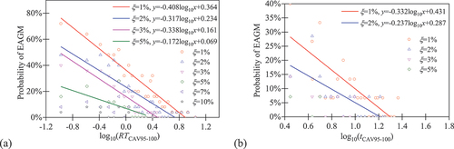
Based on the scattered data, linear regression analysis is performed for the scattered points of different damping ratios. The coefficients of the logarithm functions are shown in Figure 9(a,b). Note that to conduct a linear regression analysis, only the cases with p-values of F-Statistic less than 0.05 (indicating 95% confidence of accepting linear fitting) are shown in Figure 9. They are $\xi =$1%, 2%, 3% and 5% for non-pulse-like EAGMs, and $\xi =$1% and $\xi =$2% for pulse-like ground motions. The data points for larger damping ratios are also included in the figure. However, due to the limited number of data points, linear fitting was not performed. The information of non-pulse-like EAGMs under 5% damping ratio and pulse-like EAGMs under 2% damping ratio can be found in Appendix B. Figure 9(a) shows that the probability of non-pulse-like EAGMs generally reduces with RT_CAV95–100 and damping ratios. Based on the regression equation, zero probability of non-pulse-like EAGMs is predicted when RT_CAV95–100 exceeds 7.35 s, 4.32 s, 3.09 s and 2.75 s for $\xi =$1%, 2%, 3% and 5%, respectively. For pulse-like ground motions, zero probability of EAGMs is predicted as t_CAV95–100 >19.9 s for $\xi =$1% and 16.25 s for $\xi =$2%. Extended analysis is recommended for ground motions with the metrics within these threshold values.

5.2. Prediction of structural period windows of EAGMs

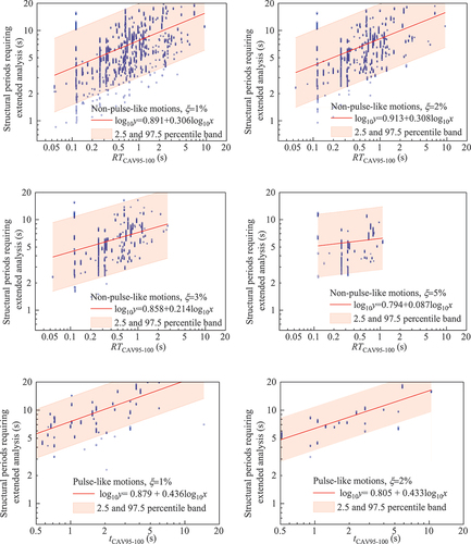
Whether an extended analysis should be conducted is unknown before conducting a structural dynamic analysis. Hence, regression analysis is performed to predict the structural period windows that require extended analysis based on the most suitable metrics. The structural periods requiring extended analysis are plotted in logarithmic coordinates to associate with the metrics of ground motions. Linear fitting is performed between the logarithmic values of structural periods and the logarithmic values of metrics, as shown in Figure 10. A general view shows that the structural periods requiring extended analysis increase with the metrics for both non-pulse-like and pulse-like ground motions, and the 2.5 and 97.5 percentile band would cover the structural periods that require extended analysis in most cases.

Figure 10. Regression analysis of structural periods that require extended analysis.

6. Conclusions

This study systematically investigates the occurrence of the absolute maximum responses (AMR) of single-degree-of-freedom systems in the post-shaking phase of sinusoidal waves and real earthquake ground motions. The characteristics of earthquake ground motions requiring extending analysis (EAGMs) are investigated and the probability of EAGMs as well as the period window are analysed. The result has important implications for calculating response spectra or conducting response history analyses with real ground motions. The key findings are summarised as follows:

1. Illustrated using a simple sine wave, it is revealed that the mechanism of the occurrence of AMR in the post-shaking phase lies in the ‘phase lag’ effect between the input ground motion and the development of the structural response. This is governed by the counteraction between the resonant effect and the damping effect. For long-period structures, the input ground motion ceased before the structure developed a full response to reach the AMR. Post-shaking analysis is more important when calculating acceleration and displacement spectra of long-period structures with low damping ratios.

2. Non-pulse-like EAGMs can be attributed to the large shaking intensity within the post-significant duration phase or the length of the post-significant duration phase is too short for reaching AMR, while the main reason for pulse-like EAGMs is the short length of the post-significant duration. RT_CAV95-100 and t_CAV95-100 are identified to best describe non-pulse-like and pulse-like EAGMs, respectively.

3. The probability of EAGMs and the structural period windows requiring extended analysis are shown based on the most suitable metrics for describing EAGMs. Based on regression analysis, threshold values for the probability of EAGMs and the bands of structural periods requiring extended analysis are determined, which would provide some guidance for structural response history analysis of earthquake ground motions.

Disclosure statement

No potential conflict of interest was reported by the author(s).

Additional information

Funding

This research is supported by the University Scientific Research Project of Guangzhou Education Bureau (No. 202032797), the Education Department of Guangdong Province (No. 2022GXJK294), and the National Natural Science Foundation of China (No. 52108445). These supports are gratefully acknowledged.

Appendices Appendix A

RSN of ground motion records selected from the PEER NGA-West2 database:

• Non-pulse-like ground motion records

3, 4, 5, 7, 8, 9, 10, 11, 12, 14, 15, 16, 17, 19, 20, 25, 32, 34, 35, 36, 42, 44, 45, 46, 47, 48, 49, 51, 56, 57, 58, 59, 62, 63, 64, 65, 68, 69, 70, 72, 73, 79, 80, 81, 82, 83, 87, 88, 89, 91, 92, 93, 94, 101, 103, 104, 105, 121, 122, 123, 131, 135, 137, 138, 139, 140, 151, 152, 153, 155, 163, 166, 169, 172, 176, 186, 188, 190, 191, 194, 196, 197, 210, 212, 213, 216, 217, 218, 220, 224, 228, 229, 246, 247, 268, 280, 281, 282, 283, 286, 287, 288, 290, 291, 293, 294, 295, 298, 299, 570, 571, 572, 573, 574, 575, 576, 577, 579, 580, 581, 582, 583, 584, 832, 835, 836, 841, 844, 847, 850, 854, 855, 856, 858, 859, 860, 861, 862, 870, 874, 880, 881, 882, 884, 885, 888, 890, 895, 897, 1144, 1149, 4061, 4062, 4063, 4064, 4066, 4067, 4068, 4069, 4070, 4071, 4072, 4074, 4075, 4076, 4077, 4078, 4079, 4080, 4081, 4082, 4460, 4461, 4462, 4463, 4464, 4465, 4466, 4467, 4468, 4469, 4470, 4471, 4472, 4473, 4474, 4475, 4476, 4477, 4478, 4479, 4481, 4840, 4841, 4842, 4843, 4844, 4845, 4846, 4848, 4849, 4850, 4851, 4852, 4853, 4854, 4855, 4856, 4857, 4858, 4859, 4860, 4861, 6879, 6881, 6882, 6884, 6885, 6886, 6888, 6889, 6890, 6891, 6892, 6893, 6894, 6895, 6896, 6898, 6899, 6900, 6901, 6902, 6903, 8056, 8057, 8058, 8059, 8060, 8061, 8062, 8063, 8064, 8065, 8066, 8067, 8068, 8069, 8070, 8071, 8072, 8073, 8074, 8075, 8076.

• Pulse-like ground motion records

77, 143, 147, 148, 149, 150, 159, 161, 170, 171, 173, 178, 179, 180, 181, 182, 184, 185, 285, 292, 316, 451, 459, 566, 568, 569, 722, 723, 764, 766, 767, 802, 828, 838, 879, 900, 982, 983, 1004, 1013, 1044, 1045, 1050, 1051, 1052, 1054, 1063, 1084, 1085, 1086, 1106, 1114, 1119, 1120, 1148, 1161, 1165, 1176, 1182, 1193, 1244, 1402, 1475, 1476, 1477, 1478, 1479, 1480, 1481, 1482, 1483, 1485, 1486, 1487, 1489, 1491, 1492, 1493, 1496, 1498, 1501, 1502, 1503, 1505, 1510, 1511, 1515, 1519, 1528, 1529, 1530, 1531, 1548, 1550, 1602, 2114, 2734, 3473, 3475, 3548, 3965, 4040, 4065, 4097, 4098, 4100, 4101, 4102, 4103, 4107, 4113, 4115, 4126, 4211, 4228, 4451, 4458, 4480, 4482, 4483, 4847, 6887, 6897, 6906, 6911, 6927, 6928, 6942, 6959, 6960, 6962, 6966, 6969, 6975, 8119, 8123, 8161, 8164, 8606.

Appendix B

Table B1 Ground motions classified as EAGM for acceleration response.

RSN	Components	Earthquake Name	Year	Station Name	Mw	Earthquake	Rrup (km)
Non-pulse-like EAGMs under 5% damping ratio
48	V	Lytle Creek	1970	Puddingstone Dam (Abutment)	5.33	Reverse Obl.	30.02
58	V	San Fernando	1971	Cedar Springs Pumph.	6.61	Reverse	92.59
62	V	San Fernando	1971	Colton-So Cal Edison	6.61	Reverse	96.81
64	H2	San Fernando	1971	Fort Tejon	6.61	Reverse	61.64
89	V	San Fernando	1971	Tehachapi Pump	6.61	Reverse	63.79
92	H2, V	San Fernando	1971	Wheeler Ridge-Ground	6.61	Reverse	70.23
94	H1, H2, V	San Fernando	1971	Wrightwood-6074 Park	6.61	Reverse	62.23
139	H1	Tabas, Iran	1978	Dayhook	7.35	Reverse	13.94
188	H2	Imperial Valley-6	1979	Plaster City	6.53	Strike slip	30.33
213	V	Livermore-01	1980	Fremont-Mission SJ	5.8	Strike slip	35.68
217	V	Livermore-02	1980	APEEL 3E HCSUH	5.42	Strike slip	30
268	H2	Victoria Mexico	1980	SAHOP Casa Flores	6.33	Strike slip	39.3
280	H1, H2	Trinidad	1980	Rio Dell Overpass FF	7.2	Strike slip	76.26
281	H2	Trinidad	1980	Rio Dell Overpass EG	7.2	Strike slip	76.26
282	H1, H2	Trinidad	1980	Rio Dell Overpass WG	7.2	Strike slip	76.26
847	H1, H2, V	Landers	1992	Compton-Castl. St.	7.28	Strike slip	161.23
856	H2	Landers	1992	Fountain Valley-Euclid	7.28	Strike slip	146.89
874	H1, V	Landers	1992	LB-Orange Ave	7.28	Strike slip	160.85
4079	V	Parkfield-02	2004	Buttonwillow - Hwy 58 & Wasco	6.0	Strike slip	85.63
4080	H1	Parkfield-02	2004	San Luis Obispo - LLG	6.0	Strike slip	61.69
8074	H2	Christchurch	2011	DORC	6.2	Reverse Obl.	60.28
Pulse-like EAGMs under 2% damping ratio
77	V	San Fernando	1971	Pacoima Dam	6.61	Reverse	1.81
147	V	Coyote Lake	1979	Gilroy Array #2	5.74	Strike slip	9.02
149	H1	Coyote Lake	1979	Gilroy Array #4	5.74	Strike slip	5.7
722	H1	Superstition Hills	1987	Kornbloom Road	6.54	Strike slip	18.48
723	H1	Superstition Hills	1987	Parachute Test Site	6.54	Strike slip	0.95
1045	V	Northridge-01	1994	Newhall - WPCRd	6.69	Reverse	5.48
1063	H2	Northridge-01	1994	Rinaldi Receiving Sta	6.69	Reverse	6.5
1148	H1,V	Kocaeli	1999	Arcelik	7.51	Strike slip	13.49
1161	H2,V	Kocaeli	1999	Gebze	7.51	Strike slip	10.92
1165	V	Kocaeli	1999	Izmit	7.51	Strike slip	7.21
1402	H1	Chi-Chi	1999	NST	7.62	Reverse Obl.	38.42
4097	H1	Parkfield-02	2004	Slack Canyon	6.0	Strike slip	2.99
4102	H1	Parkfield-02	2004	Parkfield – Chol. 3W	6.0	Strike slip	3.63

References

- Ancheta, T. D., R. B. Darragh, J. P. Stewart, E. Seyhan, W. J. Silva, B. S.-J. Chiou, and J. L. Donahue. 2014. “NGA-West2 Database.” Earthquake Spectra 30 (3): 989–1005. https://doi.org/10.1193/070913EQS197M.
- Arias, A. 1970. A Measure of Earthquake Intensity. Santiago de Chile: Massachusetts Inst. of Tech., Cambridge. Univ. of Chile.
- ASCE/SEI (American Society of Civil Engineers/Structural Engineering Institute). 2007. ASCE/SEI 7-22 Minimum Design Loads and Associated Criteria for Buildings and Other Structures. Reston, VA: The American Society of Civil Engineers.
- Bernal, D., M. Döhler, S. M. Kojidi, K. Kwan, and Y. Liu. 2015. “First Mode Damping Ratios for Buildings.” Earthquake Spectra 31 (1): 367–381. https://doi.org/10.1193/101812EQS311M.
- Bommer, J. J., and A. Martínez-Pereira. 1999. “The Effective Duration of Earthquake Strong Motion.” Journal of Earthquake Engineering 3 (02): 127–172. https://doi.org/10.1080/13632469909350343.
- CEN. 2004. EN 1998-1: Design of Structures for Earthquake Resistance. Part 1: General Rules, Seismic Actions and Rules for Buildings. Brussels, Belgium: European Committee for Standardization (CEN).
- Chopra, A. 2023. Dynamics of Structures: Theory and Applications to Earthquake Engineering. 6th ed. New Jersey: Prentice Hall.
- Cruz, C., and E. Miranda. 2017. “Evaluation of Damping Ratios for the Seismic Analysis of Tall Buildings.” Journal of Structural Engineering 143 (1): 04016144. https://doi.org/10.1061/(ASCE)ST.1943-541X.0001628.
- Elmenshawi, A., M. Sorour, A. Mufti, L. G. Jaeger, and N. Shrive. 2010. “Damping Mechanisms and Damping Ratios in Vibrating Unreinforced Stone Masonry.” Engineering Structures 32 (10): 3269–3278. https://doi.org/10.1016/j.engstruct.2010.06.016.
- Fayaz, J., M. Medalla, and F. Zareian. 2020. “Sensitivity of the Response of Box-Girder Seat-Type Bridges to the Duration of Ground Motions Arising from Crustal and Subduction Earthquakes.” Engineering Structures 219:110845. https://doi.org/10.1016/j.engstruct.2020.110845.
- Gimsing, N. J., and C. T. Georgakis. 2012. Cable Supported Bridges: Concept and Design. 3rd ed. London, United Kingdom: John Wiley & Sons Ltd. https://doi.org/10.1002/9781119978237.
- Hou, H., and B. Qu. 2015. “Duration Effect of Spectrally Matched Ground Motions on Seismic Demands of Elastic Perfectly Plastic SDOFS.” Engineering Structures 90:48–60. https://doi.org/10.1016/j.engstruct.2015.02.013.
- Kiani, J., C. Camp, and S. Pezeshk. 2017. “Role of Conditioning Intensity Measure in the Influence of Ground Motion Duration on the Structural Response.” Soil Dynamics and Earthquake Engineering 104:408–417. https://doi.org/10.1016/j.soildyn.2017.11.021.
- Kolli, M. K., and S. S. Bora. 2021. “On the Use of Duration in Random Vibration Theory (RVT) Based Ground Motion Prediction: A Comparative Study.” Bulletin of Earthquake Engineering 19 (3): 1687–1707. https://doi.org/10.1007/s10518-021-01052-w.
- Li, Z., M. Q. Feng, L. Luo, D. Feng, and X. Xu. 2018. “Statistical Analysis of Modal Parameters of a Suspension Bridge Based on Bayesian Spectral Density Approach and SHM Data.” Mechanical Systems and Signal Processing 98:352–367. https://doi.org/10.1016/j.ymssp.2017.05.005.
- Lilliefors, Hubert W. 1967. “On the Kolmogorov-Smirnov Test for Normality with Mean and Variance Unknown.” Publications of the American Statistical Association 62 (318): 399–402. https://doi.org/10.1080/01621459.1967.10482916.
- Lopes, R. H. C., P. R. Hobson, and I. D. Reid. 2008. “Computationally Efficient Algorithms for the Two-Dimensional Kolmogorov–Smirnov Test.” Journal of Physics: Conference Series 119 (4): 042019. https://doi.org/10.1088/1742-6596/119/4/042019.
- McCann, Martin W., and Haresh C. Shah. 1979. “Determining Strong-Motion Duration of Earthquakes.” Bulletin of the Seismological Society of America 69 (4): 1253–1265.
- PEER. 2017. “Guidelines for Performance-Based Seismic Design of Tall Buildings.” Pacific Earthquake Engineering Center (PEER) Report No. 2017/06, University of California, Berkeley.
- Reed, J. W., and R. P. Kassawara. 1990. “A Criterion for Determining Exceedance of the Operating Basis Earthquake.” Nuclear Engineering and Design 123 (2–3): 387–396. https://doi.org/10.1016/0029-5493(90)90259-Z.
- Shang, Q., J. Li, and T. Wang. 2022. “Floor Acceleration Response Spectra of Elastic Reinforced Concrete Frames.” Journal of Building Engineering 45:103558. https://doi.org/10.1016/j.jobe.2021.103558.
- Song, P. S., J. C. Wu, S. Hwang, and B. C. Sheu. 2005. “Statistical Analysis of Impact Strength and Strength Reliability of Steel–Polypropylene Hybrid Fiber-Reinforced Concrete.” Construction & Building Materials 19 (1): 1–9. https://doi.org/10.1016/j.conbuildmat.2004.05.002.
- Standards Australia. 2007. AS1170.4 Structural Design Actions, Part 4: Earthquake Actions in Australia. Sydney, Australia: Standards Australia.
- Standards New Zealand. 2004. NZS1170.5 Structural Design Actions, Part 5: Earthquake Actions‐New Zealand. Wellington, New Zealand.
- Tang, Y., N. Lam, and H.-H. Tsang. 2021. “A Computational Tool for Ground- Motion Simulations Incorporating Regional Crustal Conditions.” Seismological Research Letters 92 (2A): 1129–1140. https://doi.org/10.1785/0220200222.
- Tsang, H. H., E. F. Gad, J. L. Wilson, J. W. Jordan, A. J. Moore, and A. B. Richards. 2018. “Mine Blast Vibration Response Spectrum for Structural Vulnerability Assessment: Case Study of Heritage Masonry Buildings.” International Journal of Architectural Heritage 12 (2): 270–279. https://doi.org/10.1080/15583058.2017.1406015.
- Yi, J., and H.-H. Tsang. 2023. “Significance of Post-Shaking Response of SDOF Systems.” Soil Dynamics and Earthquake Engineering 173:108102. https://doi.org/10.1016/j.soildyn.2023.108102.