
Abstract
Interest rate risk is immanent to all sorts of bonds with a fixed interest rate and has a major impact on the value of the bond. The aim of this article is to evaluate this risk over a period of five years (2008–2012), applying the delta-normal Value-at-Risk (VaR) method to a portfolio consisting of bonds that were continuously traded at the Belgrade Stock Exchange and to assess the accuracy of the method for different confidence levels in that period. The results demonstrated that the method underestimated the risk for the confidence levels of 99.5% and 99% and overestimated the risk for the confidence level of 90%.
1. Introduction
Risk management represents the core activity for financial institutions operating in the financial market. Whether the financial institutions are passively accepting financial risks or trying to achieve a competitive advantage by exposing themselves to financial risks within reasonable limits, these risks should be carefully appraised due to their potential danger of causing losses. When the core activity of a business is to hold portfolios of assets, it would be dangerous to ignore their potential change in value (Koenig, 2004).
Financial institutions in Serbia invest a certain amount of their financial assets in bonds that are continuously traded at the Belgrade Stock Exchange. Interest rate risk is immanent to all sorts of bonds with a fixed interest rate. It has a major impact on the value of the bond. Interest rate risk a risk to the earnings or market value of a portfolio due to uncertain future interest rates. Changes in market interest rates affect bond prices change inversely. For market risk evaluation and analysing of such risks various models are used. One of the models is the Value-at-Risk (VaR) model.
During the 1980s, large financial institutions (Bankers Trust, Chase Manhattan Bank, Citibank and others) began applying the VaR method in risk management systems. To implement this concept, a large amount of mutually interchangeable data was required, which was a huge problem until the appearance of RiskMetrics. RiskMetrics was a free service offered by JP Morgan in 1994, to promote VaR as a risk measurement tool. It consists of detailed technical documentation, as well as the covariance matrix for several hundred key points, which were updated daily. Since JP Morgan’s Riskmetrics were published in 1994, there was a swift expansion of research into VaR methodology. While the basic concepts surrounding Value-at-Risk are founded in the area of market risk measurement they have been extended, over the last decade, to other areas of risk management. In particular, Value-at-Risk models are now commonly used to measure both credit and operational risks. (Allen, Boudoukh, & Saunders, Citation2004)
The VaR measures the worst expected loss over a given time interval under normal market conditions at a given confidence level (Dowd, Citation1998). Based on firm scientific foundations, VaR provides users with a summary measures of market risk. VaR is method of assessing risk that uses standard statistical techniques routinely used in other technical fields (Jorion, Citation2001). For instance, a company might say that the daily VaR of its trading portfolio is $20 million at the 99% confidence level. In other words, there is only 1% probability under normal market conditions, for a loss greater than $20 million to occur. VaR measures risk using the same measurement units as banks – e.g., dollars. Shareholders and managers may decide whether they consider a given risk level appropriate. In case they are not comfortable with the preferred risk level, the very process leading to VaR calculations may be utilised to make a decision on risk mitigation. Although it virtually always represents a loss, VaR is conventionally reported as a positive number. A negative VaR would imply the portfolio has a high probability of making a profit, for example a one-day 5% VaR of negative $1 million implies the portfolio has a 95% chance of making $1 million or more over the next day (Crouhy, Mark, & Galai, Citation2001).
Financial institutions developed VaR as a general measure of economic loss, which may correspond both to the risk of individual items and the aggregate portfolio risk. The VaR approach originated as a methodology for market risk measurement, but the possibility of wider application was soon perceived. Besides the mentioned primary function, VaR methodology may also be used to make investment decisions by reevaluating the yield to risk relationship, ensuring a more consistent and integrated risk management. It was likewise understood that VaR methodology may be implemented to measure and manage other kinds of risk such as: liquidity risk, credit risk, cash flow risk, and even some of the operating and legal risks. In short, VaR creates possibilities for new approaches to comprehensive risk management.
The first step towards VaR measurement is to select two quantitative factors: the holding period and the confidence level.
The usual holding period is a day or a month, but institutions may choose other periods (e.g., a quarter or more), depending on their investments and reporting periods. The holding period may also depend on the liquidity of the markets in which an institution operates. All other things being equal, the ideal holding period in any market is the time required to ensure uniform liquidation of the market positions. The more liquid the risk, the shorter the time period over which the risk needs to be assessed, i.e. the shorter the risk horizon for the VaR model. (Alexander, Citation2008). The holding period may also be specified by regulations. According to the Basel Agreement, the rules on capital adequacy demand that the internal evaluation models used to determine the minimum regulatory capital for market risk must reflect a time horizon of two weeks (i.e., 10 working days). Selection of the holding period may also depend on the following factors: the assumption that the portfolio does not change over the holding period is easier to uphold with a shorter holding period; for model validation, so-called backtesting, a short holding period is more desirable. Reliable validation requires a large data-set and a large data-set requires a short holding period. The commercial banks currently have daily VaR reports due to the fast turnover of their portfolios. In contrast, investment portfolios such as pension funds slowly adjust their risk exposure, and hence a one month period is usually chosen for their investment purposes.
The selection of confidence level depends mostly on the purpose behind the risk measurement. Therefore, a very high confidence level, often as great at 99.97%, is appropriate if used for risk measurement in order to set capital requirements or in order to achieve a low insolvency probability or high credit rating. This choice should reflect the level of a company’s aversion towards risk and expenses due to losses caused by exceeding the VaR. The larger the aversion towards risk or expense, the greater the amount of capital required to cover potential losses, which leads to a higher level of confidence. On the other hand, to validate a model, it is desirable to have relatively low confidence levels, in order to obtain a reasonable proportion of observed losses. In contrast, if VaR is only used by companies to compare the risks in various markets, then the selection of confidence level is irrelevant.
Thus, the best choice of these parameters depends on the context. It is important to make clear choices in each context and to be completely clear throughout an institution for these choices, so that setting constraints and making other decisions connected to risk may be made in light of this understanding.
2. Calculating VaR values by applying the delta-normal method
There is an inverse relationship between bond prices and interest rates, and interest rates may change significantly. A decline (rise) in interest rates will cause a rise (decline) in bond prices, with the most volatility in bond prices occurring in longer maturity bonds and bonds with low coupons (Fabozzi et al., Citation2006). The sensitivity of bond prices to changes in interest rates is very important for investors. With the rise and fall of interest rates bondholders realise capital gains or losses. That is why the investments in securities with fixed income are risky, even when the coupon payments and the principal is guaranteed.
Duration (D) is an indicator of bond’s risk because it allows to measure how sensitive the price of that bond is to changes in the market yield rate (Resti & Sironi, Citation2007).(1)
where T is number of time periods, t is respective time period, P is the current price of that bond, CF is cash flow and r is the market yield rate.
Using the link between the price of a bond (P), cash flow (CF) and yield to maturity requested by market (r) as a starting point:(2)
where T is number of time periods, we can come up with the following analytical relationship by deriving with respect to the yield rate:(3)
From it follows that:(4)
Dividing both sides by P gives us:(5)
And consequently:(6)
The expression is called modified duration; it enables us to quantify the percentage change in price that would result from an extremely small change in the market yield. If finite changes in the yield rate (Δr) are considered, instead provides an approximate estimate of the consequent percentage change in price:
(7)
Since the impact of changes in the yield rate on the market value of the bond is required, the above expression can be represented as follows:
(8)
where MVis market value of the bond, and MDis modified duration of the bond. It follows that the change in the market value of bond is:
(9)
Using delta - normal method the VaR value is calculated as follows:
(10)
where σ - the relevant market factor’s estimated return volatility, a scaling factor α which – given the hypothesis of normal distribution of market factor returns – allows to obtain a risk measure corresponding to the desired confidence level (for instance α=2 for 97.7% confidence level).
If Δr is replaced by the product of α and σ, and the loss in absolute value is considered, the following will be obtained:
(11)
To derive the formula for calculation of the VaR of a portfolio, results from standard portfolio theory are used. The continuous return on a two-asset portfolio can be written as follows:
(12)
where w represents the weight of the first asset and (1-w) is the fraction of the portfolio invested in the second asset. The variance of the portfolio is:
(13)
where - are the variances on the portfolio, asset 1 and asset 2, respectively and σ1,2 is the covariance between asset 1 and 2 returns. Restating equation (Equation12
(12) ) in terms of standard deviation (recall that
) results in:
(14)
where ρ1,2 - is the correlation between assets 1 and 2. However, the percentage VaR5% can be stated as 1.645σp. Moreover, the 5% percentage VaR for asset 1 (asset 2) can be denoted as %VaR1 (%VaR2) and can be expressed as 1.645σ1 (1.645σ2). Substituting the expressions for %VaRp, %VaR1 and %VaR2 into equation (Equation13(13) ) and multiplying both sides by 1.645 yields the portfolio’s percentage VaR as follows:
(15)
Equation (Equation14(14) ) represents the formula for the percentage VaR for a portfolio consisting of two assets. If the above applied to the portfolio of N elements, the return of the portfolio rp could be expressed as follows:
(16)
where wi represents the weight of the asset i and ri represents the return of the asset i.
The variance on the portfolio would be equal to:
(17)
or in matrix form:(18)
3. General sample information and results of applying the basic delta-normal method for estimating the VaR values for Serbian government bond portfolio
In this article VaR is calculated for confidence levels of 90%, 95%, 99% and 99.5%, for a one-day prediction period, by applying the basic delta-normal method to portfolio consisting of four bonds that were continuously traded at the Belgrade Stock Exchange, for a period of five years (01.01.2008.-31.12.2012.).
Data were taken from the website of the Belgrade Stock Exchange – www.belex.rs. The following zero-coupon bonds: A2013, A2014, A2015, A2016, are examined. Dates of maturity for this bonds are shown in Table .
Table 1. Dates of maturity for bonds.
The underlying assumption is that the bond shares in portfolio are equal:(19)
Then the 1,262 consecutive VaR values are estimated on the basis of data on 250 consecutive value changes (one year) of the portfolio. The results are shown in Table and Figures .
Table 2. Calculated VaR values by applying delta-normal method on the different dates, for different confident levels.
Figure 1. Graphical representation of the portfolio returns and VaR values obtained by applying delta-normal method for portfolios of bonds traded on the market of the Republic of Serbia, for confidence level of 99.5%, for the period 2008–2012. Source: Created by the authors.
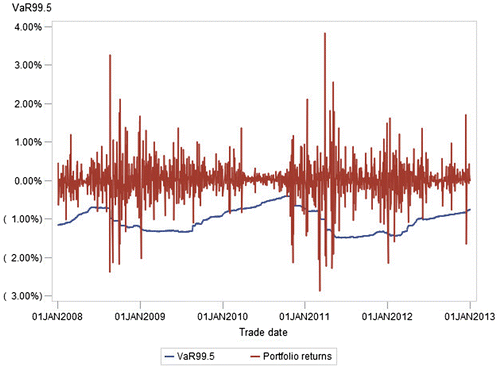
Figure 2. Graphical representation of the portfolio returns and VaR values obtained by applying delta-normal method for portfolios of bonds traded on the market of the Republic of Serbia, for confidence level of 99%, for the period 2008–2012. Source: Created by the authors.
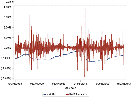
Figure 3. Graphical representation of the portfolio returns and VaR values obtained by applying delta-normal method for portfolios of bonds traded on the market of the Republic of Serbia, for confidence level of 95%, for the period 2008–2012. Source: Created by the authors.

Figure 4. Graphical representation of the portfolio returns and VaR values obtained by applying delta-normal method for portfolios of bonds traded on the market of the Republic of Serbia, for confidence level of 90%, for the period 2008–2012. Source: Created by the authors.
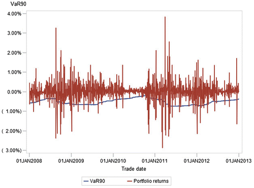
The chart shows that the portfolio returns were much more variable during 2008 and 2011, which influenced the calculated VaR values in the tables on 31.12.2008 and 31.12.2011. Consequently, the mentioned values were 30–80% higher than the VaR values in other years. In 2008 the global economic crisis began, while judging from the market data, the second wave of crisis in Serbia began in 2011.
4. Verification of the accuracy of the model
Estimated VaR values should not be taken for granted. From the above it can be seen that the returns of the portfolio on some days exceeded the estimated value of the portfolio VaR. Therefore verification of the accuracy of the model should be carried out.
The easiest way to verify the accuracy of the model is to record the failure rate, which gives the proportion of the number of times the VaR exceeded expectations in a given sample. Assume that N is the number of times the loss is exceeds. At a given confidence level, N can be too small or too large. The following Table shows how often the loss was greater than anticipated VaR value, for a given level of reliability for years 2008–2012 where T – total number of consecutive VaR predictions, and N – number showing how many times the actual loss exceeded the VaR from the previous day.
Table 3. Review of the calculated values – how many times the actual loss exceeded the previous day VaR value for a portfolio consisting of bonds traded on the market of the Republic of Serbia, using the delta-normal method, for each year and for the entire period 2008–2012.
Once the failure rate is calculated as N/T and compared to the left tail probability, e.g., p = 0.01, which is used to determine VaR evaluation, if they match the VaR evaluation was correct, and if they differ significantly the model has to be rejected.
For the sake of illustration, the confidence level is set at 95%. This number does not refer to the quantitative level p that was selected as the VaR, which might be p = 0.01 for instance. This confidence level refers to the decision on whether to reject the model or not. It is generally set at 95% because this corresponds to two standard deviations under a normal distribution.
Kupiec (Citation1995) developed the confidence regions for such a test. These regions are defined by the tail points of likelihood ratio:(20)
which is distributed through χ2 test with one degree of freedom under the null hypothesis that p is a true probability.
For example, in a sample consisting of 250 data (T = 250) one might expect to observe deviation. However, the null hypothesis can’t be rejected as long as N is within the confidence interval [15 < N < 35]. Values of N greater or equal to 35 suggest that VaR model represents the probability of large losses lower than it actually is; values of N that are less than or equal to 15 suggest the VaR model is too conservative. The following Table shows the regions in which the model is not rejected on the basis of significance α = 0.05.
Table 4. Model verification: regions in which the model is not rejected at the significance level of 0.05.
The following Table presents whether a model is acceptable or not, on the basis of Kupiec likelihood ratio.
Table 5. Model verification for a portfolio consisting of bonds traded on the market of the Republic of Serbia, using the delta-normal method, for different confidence levels, for each year and for the entire period 2008–2012.
5. Conclusion
VaR forecasts are of great importance for financial and risk management. The relative literature includes a variety of different methods. In this article, VaR is calculated for confidence levels of 90%, 95%, 99% and 99.5%, for a one-day prediction period, by applying the basic delta-normal method to portfolio consisting of four bonds that were continuously traded at the Belgrade Stock Exchange, for the period of five years (01.01.2008–31.12.2012).
Verification of the accuracy of the model has been done on the basis of significance α = 0.05 and results demonstrated that the method underestimated the risk for the confidence levels of 99.5% and 99% and overestimated the risk for the confidence level of 90%. The model can be accepted only for the confidence level of 95%.
Disclosure statement
No potential conflict of interest was reported by the authors.
References
- Alexander, C. (2008). Market risk analysis, volume IV: Value at risk models. Chichester: John Wiley & Sons Inc.
- Allen, L., Boudoukh, J., & Saunders, A. (2004). Understanding market, credit, and operational risk: The value at risk approach. Malden:Wiley –Blackwell.
- Crouhy, M., Mark, R., & Galai, D. (2001). Risk management. New York, NY: McGraw-Hill.
- Dowd, K. (1998). Beyond value at risk, The new science of risk management. West Sussex, England: John Wiley & Sons Ltd.
- Fabozzi, F. J., Martellini, L., & Priaulet, P. (2006). Advanced bond portfolio management. Hoboken, New Jersey: John Wiley & Sons Inc.
- Jorion, P. (2001). Value at risk. New York, NY: McGraw-Hill.
- Koenig, D. R. (2004). Volume III: Risk management practices. Wilmington, DE: PRMIA Publications.
- Kupiec, P. (1995). Techniques for verifying the accuracy of risk measurement models. The Journal of Derivatives, 3, 73–84.10.3905/jod.1995.407942
- Resti, A., & Sironi, A. (2007). Risk management and shareholders’ value in banking: From risk measurement models to capital allocation policies. West Sussex, England: John Wiley & Sons Ltd.