Practical aspects of portfolio selection and optimisation on the capital market

Abstract

This article highlights some observations concerning the deficiencies in the application of statistics on the capital market, with special reference to Modern Portfolio Theory (MPT). The main point is the sensitivity of statistical parameters (especially the standard deviation of the daily rates of return) to subjective/random factors. For securities with similar patterns and quasi-identical charts, statistical results in contradiction to the evidence of the market can be obtained. This article makes a pledge in favour of the necessity for increased attention in constructing an optimal/efficient portfolio.

Keywords:

• Stock exchange
• statistics
• technical analysis
• Modern Portfolio Theory (MPT)

JEL classification:

• G11
• G14
• G15
• G17
• G23

1. Introduction

For any investor and/or stock market speculator, the first thing taken into consideration is the return on investment and the associated risk. The No Arbitrage principle stipulates No Free Lunch (Arratia, 2014), meaning that money cannot be made of thin air (without an initial investment). Equally, you cannot earn money without risk, hence, the risk increases with the expected profits for securities located on the efficient frontier.

According to Modern Portfolio Theory (MPT), in order to create an optimal/efficient portfolio, a selection method is used based on statistical considerations of the rate of return, risk, and the correlation of securities. Securities can be stocks, bonds, indexes, futures/options, structured products, commodities, currencies; practically any asset traded to allow precise determination of rate of returns, on a predetermined time frame. The asset diversification of a portfolio aims at reducing non-systemic risks that are specific to a particular issuer or market.

Let Y₀, Y₁,…, Y_k,…, Y_T-1, Y_T, with T ≥ 2, closing values of asset Y, traded on a market. Values can be daily, weekly, monthly, yearly, as long as they are available regularly and periodically.

For the time frame (interval) [0,T], a characterisation of the evolution of the asset is made through:

-	Periodic-time valuation of the average rate of return, assimilated to order I moment, attached to random variable that models the temporary evolution of the rate of return; and
-	Momentary-periodic valuation of the dispersion of rate of return, assimilated to order II moment, of the random variable,

so by knowing/valuating main statistical parameters of a selection.

Also it is supposedly known – possible to estimate/approximate – the probability function of the random variable that is modelling the temporary evolution of the return of the asset.

For each moment k, the rate of return in moment k, 1 < k < T, can be defined in two ways

or(1)

In the first form, the daily percentage rate of return is defined according to the daily quotations Y of current day k, compared with the previous day k-1. The second form of the equation (1), the log profitability is defined.

The second formula is a purely mathematical property of logarithms, having no sense applying logarithmic function for a physical quantity characterised by a unit of measurement. E.g., log($1)=0 ≠ log(¢100)=2, although 1 US dollar is obviously equal to 100 cents.

The probability function of the rate of returns can be considered normal – Gaussian, either lognormal, or approximated by a lognormal – log-Gaussian function. Therefore, we use the logarithmic expression, because statistically, it is necessary that a loss –x be counterbalanced by an equal and opposite gain, x, in order for the statistical mean to logically make sense. For small values of the r_k daily variation, the two rates of returns are close enough to be considered equal. For example, for daily variations of 5% between the values calculated by the two methods, there is a relative difference of only 2.42%.

2. Literature review

One aspect of managing the financial instruments portfolio is to optimise portfolio administration based on various criteria; the most commonly used one is the profitability – risk criterion. In 1952, Markovitz proved that in a perfect market context, one can determine the set of efficient portfolios that lie on a hyperbolic curve, called the efficient frontier, where each portfolio that has a required return, the risk is minimal.

Sharpe (1964), based on the capital asset pricing model(CAPM) theory, has shown that when there is a risk free active in the portfolio, the efficient frontier is a straight line which can be determined. Considering the above, each portfolio manager tries to be on the efficient frontier. Analysing the literature in the field we were able to identify some studies that supplement the results of the two Nobel laureates.

Sortino and Satchell (2001) goes beyond MPT suggesting the downside risk as a better measure for portfolios risks. He mentions some divergences between authors regarding the theoretical and/or practical aspects, most of them because of the initial assumptions.

Sortino et al. (2010) developed their theory, introducing upside potential and the Desired Target Return. They also criticised the MPT, showing that, according to Fama, the CAPM market portfolio does not exist, no matter the value of alpha or beta considered.

Schulmerich, Leporcher, and Eu (2015) investigate the investor’s behaviour in contrast between rational and irrational (behavioural). Crises are investigated, analysing if risk measurements are correct regarding the chosen investment strategies.

Marty (2013) systematise in a mathematical matter the basics of portfolio selection and analyse.

Elton et al. (2014) state that ‘portfolio analysis is the recipe for one of the few “free lunches” in economics’. They discuss topics like market equilibrium, market efficiency, and investment valuation and analysis.

Baker and Filbeck (2013) synthesised the most recent breakthrough in portfolio theory and management, combining the theoretical background with the practical results.

Francis and Kim (2013) reviewed the relevant literature regarding MPT, as developed after Markowitz.

Sironi (2015) went beyond MPT and inspected the portfolio choice probabilistic scenario optimisation.

Our own studies, confirm the strong positive correlation between shares listed at the Bucharest Stock Exchange (BSE), making diversification less efficient against market crashes.

Levy (2012) demonstrates that CAPM must not be empirically rejected and can coexist with behavioural approaches.

Fărcaş and Cuzman (2002a, 2002b) studied the applicability of Markowitz and Sharpe’s methods on the Romanian stock market as well as the methods of optimising the rate of return based on the risk-return criterion.

Fărcaş and Fărcaş (2008) bring forth practical and empirical literature on numerical methods for optimising equity portfolios with applications on the Romanian market. The paper had presented software which permits efficient frontier numerical construction in accordance with Markowitz theory and a case study applied to Romanian Bucharest Stock Exchange (BVB) market. The conclusion of this study highlights the optimisation methods via rentability – risk criteria, and their usefulness in the investment policy of the portfolio management, considering the confidence interval and error probabilities.

Fărcaş and Deac (2010) analyse the statistical relationship of changes in share prices and their influence on decisions regarding the optimisation of portfolio management and determining the efficient frontier portfolios.

Sortino and Price (1994) developed the concept of downside risk, in order to eliminate the disadvantages of risk measurement, through the dispersion variation around the average returns of financial instruments. In our opinion, within empirical studies, on the application of optimisation theory equity portfolios, risk measurement is better represented by measuring the variation risk of dispersion of returns.

Arratia (2014) provides a qualitative overview regarding the techniques of using the statistical tools and methods available in free software R, for processing and analyzing real financial data.

Baker and Filbeck (2013) present a comprehensive analysis both for theory and practice regarding the structure, composition and optimization on an optimal portfolio.

Chen (2010) provides an important assessment regarding the technical analysis, it's principles and the basic techniques which underlies this special tactic.

Di Lorenzo (2013) presents the modern approach regarding the application of the technical analysis, especially regarding the specific protocols and techniques with a special focusing of the most efficient technical analysis queries.

Elton et. al. (2014) assess one of the most comprehensive and complex analysis upon modern portfolio theory and investment with a special focus upon the perfect balance equilibrium in modern portfolio structures.

Vollmer (2015) provides and excting overview regarding the efficient portfolio optimisation using the CAPM, with in insightfull focus on the excess returns through active investment strategies.

3. Research methodology

The main hypothesis of this study starts from the question: Why a coherent and complete theory, like MPT, does not fit with a practical result on the capital market. We have identified some of the reasons behind these weaknesses of the practical aspects of MPT.

Stock prices have been downloaded from specialised sites and taken into Microsoft Excel, as .csv or .xls files. Data processing was performed using Microsoft Excel Data Analysis module, and by using Crystal Ball, and the data was exported and processed in Mathcad or Mathlab.

The preliminary study of quotations, necessary to define the most relevant aspects of technical analysis, was performed on specialised sites, through special programs or on the stock exchanges’ websites. Technical analyses were interpreted based on a vast bibliography available in this area (Thomsett, 2012a; Chen, 2010; Murphy, 2004; Di Lorenzo, 2013).

The selection and optimisation of a portfolio of N assets is performed the classical way using MPT:

-	It is considered (Elton, 2014) a portfolio of N assets. Let xi be the share of the asset i in the structure of the considered portfolio. The weights xi satisfy the conditions:

(2)

specifying that if the market sales short, weights can also be negative.

Also, the following sizes are known (have been evaluated):

-	average rate of return of asset i, for an analysed period T;
-	σi standard deviation of i title;
-	σij covariance between the rate of return on asset i and the rate of return of asset j;
-
-	ρij Pearson correlation coefficient.

The next relations take place:(3)

For a portfolio of N assets, the average rate of return and risk are noted, respectively σ, and defined by the following relations:

Rate of return:

(4)

and Risk:(5)

Selection and determination of efficient/optimal portfolio composition, in Markowitz’s model, based on the rate of return – risk criterion, consists of determining weights x₁, x₂,…, x_N-1, x_N so that, for an imposed value of the rate of return of the portfolio the value of the associated risk should be minimal, or for given/accepted value of the risk, the value of the rate of return to be maximum.

Thus, determining the efficient/optimal portfolio composition, based on the rate of return – risk model, is made by solving the following optimisation problem:

, with restriction (6)

The above is a quadratic optimisation problem and can be solved through the method of Lagrange multipliers.

The graphical representation of the result set is the efficient frontier (Reilly & Brown, 2012; Francis & Kim, 2013), a curve, on which the most cost-effective/efficient – for a given risk – portfolio is found, respectively the least risky combination of assets that generate an expected rate of return. Although the mathematical approach is precise and rigorous, input data are estimates of statistical parameters. Hence, it starts from uncertain data, obtained with a certain level of confidence, irreproducible and affected by errors.

The optimisation problem shown in (6) is equivalent to Markowitz’s (1952) optimisation method, based on the profitability – risk criterion.

4. Results and discussions

4.1. Data series invariance in logarithmic operation

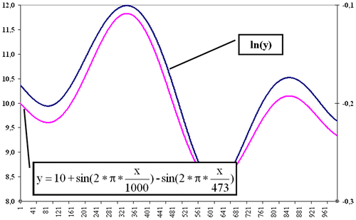
Apparently, the plot analysis will be different depending on the adopted scale: normal or logarithmic. The technical analysis (Murphy, 1999) makes a clear distinction between these two types of graphs. In Figure 1 there is a difference between the two graphs, hence, each one will have to be analysed separately.

Figure 1. Difference between a normal and logarithmic chart. Source: Authors’ estimation.

Under Association for Investment Management and Research (AIMR) standard rules, a risk measurement through the usage of standard deviation is recommended for total risk and the usage of the Sharpe’s beta coefficient as a measure of market risk. However, according to Todea (2006) logarithmic returns have the property of being additive; property which does not check in the case of arithmetic returns (of percentage variations). Furthermore, there are differences in terms of symmetry on the usage of the two methods for calculating profitability a posteriori, through the method of percentage and logarithmic variations, the second method having symmetry property.

Therefore, it would be expected that through successive logarithmic or exponential operations, the graphical method will clarify particular aspects (details) of asset evolution. This conclusion is however contradicted by a logarithmic property of the function: for cyclical functions, the normal and logarithmic charts are overlapping, if represented at appropriate scales. The example in Figure 2 is conclusive: any technical analyst will draw the same conclusions, no matter which graphics are studied.

Figure 2. Similarity of a logarithmic graph compared to a temporal one. Source: Authors’ estimation based on data collected from stooq.com.

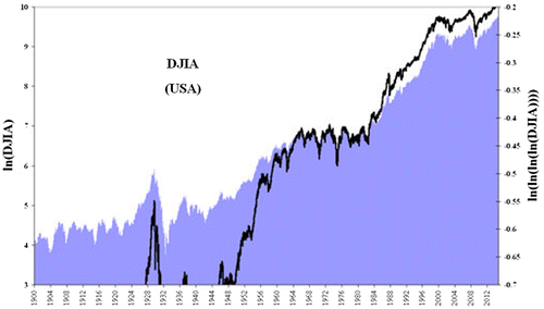
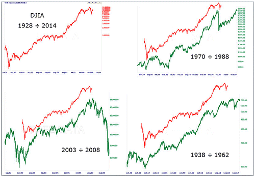
In Figure 2 we intended to highlight only one graphical aspect of technical analysis. Figure 2 has an illustrative character – intuitive in order to highlight the correlation between Dow Jones Industrial Average (DJIA) rate variation and temporal variation of the same logarithmic index.

Following empirical studies, it was found that, generally speaking, the return’s distributions are not, usually, normal or lognormal distributions. The above-mentioned studies tackles, more or less, these distributions, which enables the application of optimisation methods according to the rentability – risk criteria (Markowitz’s and Sharpe’s model). Estimating future returns can be made with reasonable confidence only if we accept the assumption of normality. Without accepting the normality hypothesis of the rate of return’s variations, future estimates must rely on other techniques, which are not part of our study.

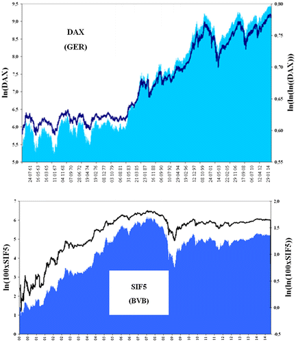
The checking of this invariance can be made by successively applying the logarithm operation to stock data series (according to Figure 3). The conclusion is valid also for other markets as shown in Figure 3 for DAX and SIF5 (Issuer from Romanian market, BVB).

Figure 3. Stock charting invariance at logarithmic operation. Source: Authors’ estimation based on data available from stooq.com and bvb.ro.

The results are as follows:

-	Through successive logarithm (exponential) operations, the technical analysis of listed assets does not improve;
-	Conclusions drawn on normal series are also available on logarithmic ones (and vice versa), the graphs being similar.

Graphic invariance of the logarithmic operation may have important consequences for some of the capital markets theories, consequences which must be deepened by subsequent studies:

-	Technical analysis deals differently with normal and logarithmic graphs. If, however, they have a similar structure, interchangeability would be one consequence, except for establishing the main trends,
-	Fractal theories are based on double logarithmic graphs, possibly with the flexibility of time scale (Mandelbrot, 2008);
-	Fractal aspects may be graphically pictured by successive logarithmic operations. Fractals are auto reproductive figures at scale, commonly found in the study of graphs, including stocks. Figure 4 shows that, without altering the time scale, the evolution of DJIA quotations, for short periods of time, are similar to long periods. The possibility that successive logarithmic operations to reveal fractal and other parties with implications for predictability, remains a study objective as well as on stock market theories in general.

Figure 4. Fractal structures in Dow Jones chart. Source: Authors’ processing.

4.2. Limitations of MPT application in practice

We will not dwell on application failures in real conditions, on the capital markets known to practitioners and mentioned on popular sites. We will only focus on those practical issues that make it difficult to use the theory models of the market even under ideal market conditions.

4.2.1. Distribution of daily rate of returns is not normal

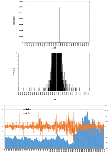
The first and most obvious shortcoming of the practical application of MPT is that the daily rates of returns are not part of a normal statistical distribution. Considering the logarithmic rate of returns of the DJIA from 1900 to the date of writing (9 October 2014), in Figure 5 we can see that the distribution is different from a normal one.

Figure 5. Statistical analysis of the daily DJIA. Source: Authors’ estimation based on data from stooq.com.

Notes: Distribution is closer to Student (top) than normal (lower). Data processed by authors in CristallBall (Oracle).

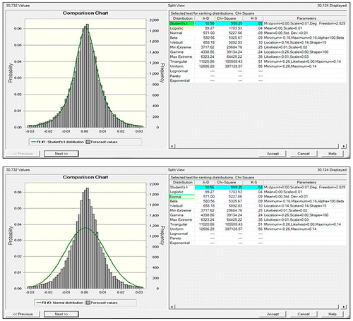
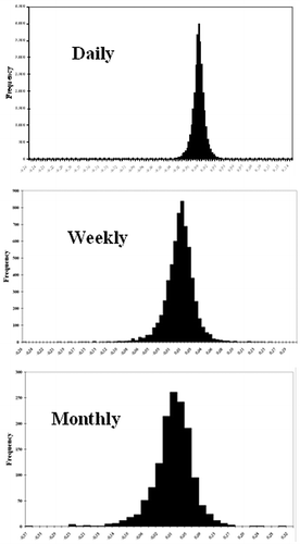
The shape of the daily distribution differs from the monthly and weekly distributions, as it is highlighted in Figure 6. Therefore, the results obtained on daily series could differ from those on longer time series. This conclusion contradicts the main assumptions of the technical analysis, on the indifference of results against the selected time interval. It also draws attention to the credibility of such statements in the technical analysis, not statistically covered.

Figure 6. Statistical series depend on samplings (the period under review). Source: Authors’ estimation based on stooq.com, from DJIA quotation series.

Courtesy access offered by the BSE, we were able to analyse all transactions on issuer SIF5, during the period 3 January 2006 to 20 January 2015. Only transactions on the Regular Market on BVB Stock Exchange (REGS) market were selected, so the statistical data base was no longer influenced by time frame. Statistical results show the majority data congested in the centre (Δ ln ≈ 0), with little data, but large values, scattered to the end (long tails) according to Figure 7.

Figure 7. Distribution of all transactions on SIF5 issuer. Source: Authors’ processing.

The implications of this result are important for capital market practitioners:

-	It shows that market movements, even the wide ones, consist of several transactions with large variations followed by stabilising the course at the new price;
-	The result demonstrates that in practice, price changes do not fall into any theoretical statistical distribution;
-	The chosen time frame is essential for establishing the statistical distribution required by MPT, which is counter-intuitive for a practitioner.

4.2.2. Daily returns statistical series

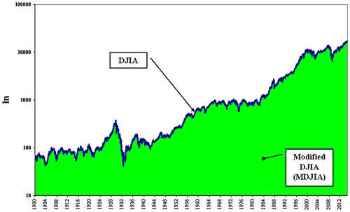
It is considered a minor modification of the series of daily quotations, so:(7)

with the new series named Modified DJIA, MDJIA.

There were permutated three successive days’ quotations, than the procedure was extended to the entire range formulas, in Microsoft Excel. As shown in Figure 8, the result (chart progress) does not change significantly. Any investor/speculator, except intraday, does not make any distinction between the two assets: DJIA and MDJIA.

Figure 8. Similar charts for DJIA and MDJIA. Source: Authors’ estimation.

Statistically speaking, permutations affect daily returns, so equation (1) is not invariant under the transformation (6). Analysing the data in Excel, the results are summarised in Table 1.

Table 1. Statistical analysis of DJIA and MDJIA.

	DJIA	MDJIA	Δ
Mean	0.000184429	0.000185583	0.63%
Standard Error	0.000064617	0.000101218	56.64%
Median	0.000484174	0.000325487	-32.77%
Standard Deviation	0.011158064	0.017478251	56.64%
Sample Variance	0.000124502	0.000305489	145.37%
Kurtosis	25.99698121	27.52381909	5.87%
Skewness	-0.818790328	-0.542106195	-33.79%
Range	0.399797287	0.669873139	67.55%
Minimum	-0.256324765	-0.366427657	42.95%
Maximum	0.143472522	0.303445482	111.50%
Sum	5.499303252	5.533699642	0.63%
Count	29818	29818

Source: Authors’ calculation based on data available from stooq.com.

The average value does not change substantially, a phenomenon easy to predict because the overall result is the same: the start and the end are the same. Instead, the standard deviation is radically different, so from the point of view of MPT, MDJIA appears much more risky than the DJIA. This is clearly contradicted in practice, however, being able to guarantee any technical analyst, on the graphic bases that both of them have equal absolute returns and risks.

Moreover, the two series give a completely surprising result: CORREL_DJIA;MDJIA = -0.0158, meaning that the two data series are uncorrelated (independent). It follows that the same data series are correlated in terms of technical analysis (intuitive), but not correlated statistically and in terms of portfolio selection based on MPT.

This result leads us to conclude that MPT has a major deficiency: it was created as a way for portfolio diversification to overcome non-systemic risks. Or, this result is missed by mathematical formalism, as demonstrated by the following argument:

Don’t put all your eggs in one basket is an idiom, including actions: if you drop the basket, all is lost. An important consequence would be the need to diversify, to disperse non-systemic risk; a prerequisite of MPT. Or, just this prerequisite is lost from the math of MPT.

From MPT it is known (Altăr, 2002) that an optimal Paretto portfolio corresponds to the following relationship between profitability and variance:

where:

, , , , , with vectors μ of yields and x of weights. It is noted that the covariance matrix Ω must be reversible, i.e., it is not allowed for securities to be perfectly correlated, positive or negative ().

Therefore, if the securities are perfectly correlated, MPT cannot make the selection, considering them identical and thus reducing the size of the matrix until it is reversed. But these securities are best suited for removing systemic risk: if an investor appreciates a security to be best suited for meeting his requirements, it will acquire spoken security. Hence, he exposes to non-systemic risks (depending only on the issuer), being exposed, for instance, to a particular problem of the issuer. But if he finds more issuers with identical risk-yield profile, he can build a diversified portfolio, in which the risk that one issuer has a problem is greatly diminished. This precise aspect is missed by the MPT, because it cannot work with the Ω singular covariance matrix.

In conclusion, a different approach to portfolio construction methodology is welcome, thanks to the theoretical and practical criticism of current theories. Standard statistical correlation imposed by the mathematical theory of MPT does not meet the needs of practitioners.

We are currently working on a new approach in what concerns the correlation measuring between two securities, based on measuring the rate of return in one security, determined by the variation of the other.

4.2.3. Implications in portfolio selection

By tracing the efficient frontier, it is confirmed that the above situation is confusing for investors.

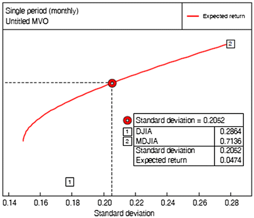
Because daily statistical data are too small, annual data were considered, namely the average and standard deviation corresponding to 256 trading days. The results were processed in VisualMVO, and then plotted in Figure 9. The absurd character of the situation is clear: although the DJIA and MDJIA are equivalent in practical terms, MPT can build an effective border, wherefrom one can choose different portfolios.

Figure 9. The DJIA+MDJIA portfolio. Source: Authors’ estimation.

Notes: Chart obtained by authors in VisualMVO. The result is not useful in practical terms, because the two titles are similar.

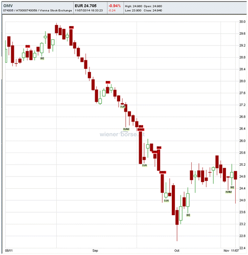
It may be objected that the example shown is unreal and specifically chosen to distort the results. For a technical analyst, using (Thomsett, 2012b) candlestick charting (see Figure 8, taken from the Wiener Börse site), the order of quotations matters; the daily quotation may not be permutated in accordance with Formula (5).

The criticism is not justified, if we analyse in detail the theoretical premises. MPT states that future estimates must be considered and not the historical values. Consider two analysts who judge a title similar evolution: they forecast MDJIA and DJIA charts, which are similar. Their findings will be divergent: only the average is the same; the dispersion and the correlation are completely different, as shown in Figure 10, where Japanese formations depend on daily price movements. Therefore, they achieve results which behave differently in terms of MPT, which contradict common sense and the practical reality.

Figure 10. Japanese formations for technical analysis. Source: Authors’ processing from data available on the Wiener Börse website.

5. Conclusion

The academic importance of the article is derived from our multiple attempts in signalling the limitations of the MPT in practice.

The practical importance of the article is derived from the observation that MPT has some limitations. We highlight some of these limitations.

Although MPT is a solid mathematical theory, its application is based on input data estimated from statistical selection of operations that can be sometimes precarious, subjective and can be easily manipulated.

In our opinion, the reasons of MPT’s practical deficiencies are:

-	Statistical consideration of returns. Based on our experience of the stock market, investors are concerned about the behaviour of the asset in relation to market trends.
-	The statistical analysis of daily returns forms a static, rigid frame, for title or market characterisation (in intermarket portfolios). In our opinion, the direction of analysis should be the mathematical dynamic expression of trends, in contrast with this static vision.
-	According to the literature and the market experience standard deviation of the return is not a proper measure of risk.
-	In a portfolio, volatility can be analysed regarding the investment period. Portfolio analysis must be performed frequently enough to cover the natural volatility of the security/market. But risk measure must also be related to trend and market crises.

The charts interpretation is straightforward, trends and sub-trends are obvious; nevertheless, their analytical description is difficult and complex. It is considered that the determination and analytical expression of the trend is a particular important problem that remains open, along with the measurement of asset’s adaptability to the overall market trends.

Based on our experience regarding stock exchange markets, we have identified some innacuracies in applying MPT in practice. Some innacuracies can appear also due to the evaluation of the linkage between titles variation throughout the covariance matrix. We consider that this method is not an efficient tool for measuring the relationship between the titles variation.

The article brings a new result about the fact that graphs remain similiar in successive logarithmic operations and show that relatively small variations of statistical values have major effects on the results of the selected securities.

The study will be continued with graphic designs for selecting weights in portfolio, with studies on the correlation between securities and other econo-physical aspects that shape the capital market by similar physical phenomena and with mathematical modelling and simulation of trends and sub-trends value of securities and market indices.

Disclosure statement

No potential conflict of interest was reported by the authors.

References

- Altăr, Moisă (2002). Portfolio theory. Romania: The Bucharest Academy of Economic Studies.
- Arratia, A. (2014). Computational finance. An introductory course with R. Barcelona: Atlantis Press. 10.2991/978-94-6239-070-6
- Baker, H. K., & Filbeck, G. (2013). Portfolio theory and management. Oxford: Oxford University Press. 10.1093/acprof:oso/9780199829699.001.0001
- Chen, J. (2010) Essentials of technical analysis for financial markets. New Jersey: John Wiley & Sons, Inc.
- Di Lorenzo, R. (2013). Basic technical analysis of financial markets. A modern approach. Milano: Springer. 10.1007/978-88-470-5421-9
- Elton, E. J., Gruber, M. J., Brown S. J., Goetzmann, W. N. (2014). Modern portfolio theory and investment analysis. ninth edition. New Jersey: John Wiley & Sons, Inc.
- Fărcaş, P., & Cuzman, I. (2002a). A selection model for efficient diversified equity portfolios. Bulletins for Applied & Computer Matematics (Bam-2035). Budapest: Pamm Centre, pp. 83–94.
- Fărcaş, P., & Cuzman, I. (2002b). Comparative study of the sharpe and markowitz methods. Part I. Methods for portfolio optimization according to the risk – rentability criteria. “Aurel Vlaicu” University of Arad Annals, Economics Series, 12, 329–335.
- Fărcaş, P., & Deac, D. (2010) Portfolio management of stocks quoted at the bucharest stock exchange and the statistical connections of the quotation variations. Studia Universitatis “Vasile Goldiș” Arad, Economics Series, Year 20/2010, Part II, 21, 167–176, Arad, Romania.
- Fărcaş, P., & Fărcaş, R.-C. (2008) Numerical methods for optimization of the financial assets portfolios. Studia Universitatis “Vasile Goldiş” Arad, IT Series, No. 1x/2008, “Vasile Goldiş” University Press. Vol. I, 150-159.
- Francis, J. C., & Kim, D. (2013). Modern portfolio theory. Foundations, analysis, and new developments. Hoboken, New Jersey: John Wiley & Sons, Inc.
- Levy, H. (2012). The capital asset pricing model in the 21st century analytical, empirical, and behavioral perspectives. Cambrigde, UK: Cambridge University Press.
- Mandelbrot, B. B. (2008). How fractals can explain what’s wrong with wall street. New York, NY: Scientific American.
- Markowitz, H. M. (1952). Portfolio selection. The Journal of Finance, 7, 77–91. doi:10.2307/2975974. JSTOR 2975974.
- Marty, W. (2013). Portfolio analytics. An introduction to return and risk measurement. Geneve: Springer International Publishing Switzerland. 10.1007/978-3-319-03509-3
- Murphy, J. J. (1999). Technical analysis of the financial markets. A comprehensive guide to trading methods and applications. New York, NY: New York Institute of Finance.
- Murphy, J. J. (2004). Intermarket analysis. Profiting from global market relationships. Hoboken, NJ: John Wiley & Sons, Inc.
- Reilly, F., & Brown, K. (2012). Investment analysis & portfolio management. Mason, OH: FinancialEbooks.net, Business School Edition.
- Schulmerich, M., Leporcher, Y.-M., & Eu, C.-H. (2015). Applied asset and risk management. A guide to modern portfolio management and behavior-driven markets. Berlin Heidelberg: Springer-Verlag. 10.1007/978-3-642-55444-5
- Sharpe, W. F. (1964). Capital asset prices: A theory of market equilibrium under conditions of risk*. The Journal of Finance, XIX No. 3, 425–442.
- Sironi, P. (2015). Modern portfolio management: From Markowitz to probabilistic scenario optimisation. Goal-Based and long-term portfolio choice. London: Incisive Media Investments Ltd.
- Sortino, A., & Price, L. (1994). Performance measurement in a downside risk framework. The Journal of Investing, 3, 59–64. doi:10.3905/joi.3.3.59.
- Sortino, F. A., & Satchell, S. E. (2001). Managing downside risk in financial markets: Theory, practice and implementation. Reed Educational and Professional Publishing Ltd.
- Sortino, F., et al. (2010). The Sortino framework for portfolio construction: Focusing on desired target return to optimize upside potential relative to downside risk. Elsevier Inc.
- Thomsett, M. C. (2012a). Bloomberg visual guide to candlestick charting. Hoboken, New Jersey: John Wiley & Sons Inc. 10.1002/9781119204923
- Thomsett, M. (2012b). Technical analysis of stock trends explained. Ethan Hathaway: An Easy-to-Understand System for Trading Successfully.
- Todea, A. (2006). Investment. selection and financing the investment projects. Financial investments – portfolio management. Cluj – Napoca: Casa Cărții de Știință Publisher.
- Vollmer, M. (2015). A beta-return efficient portfolio optimisation following the CAPM. An Analysis of International Markets and Sectors. Wiesbaden: Springer Fachmedien.10.1007/978-3-658-06634-5