Non-structural approach to implied moments extraction

Abstract

Moments of future prices and returns are not observable, but it is possible to measure them indirectly. A set of option prices with the same maturity but with different exercise prices are used to extract implied probability distribution of the underlying asset at the expiration date. The aim is to obtain market expectations from options and to investigate which non-structural model for estimating implied probability distribution gives the best fit. Non-structural models assume that only dynamics in prices is known. Mixture of two log-normals (MLN), Edgeworth expansions and Shimko’s model (representatives of parametric, semiparametric and nonparametric approaches respectively) are compared. Previous researches are inconclusive about the superiority of one approach over the others. This article contributes to finding which approach dominates. The best fit model is used to describe moments of the implied probability distribution. The sample covers one-year data for DAX index options. The results are compared through models and maturities. All models give better short-term forecasts. In pairwise comparison, MLN is superior to other approaches according to mean squared errors and Diebold-Mariano test in the observed period for DAX index options.

Keywords:

• Edgeworth expansions
• implied moments
• mixture of two log-normals
• Shimko’s model

Subject classification codes::

• C14
• C58
• G1

1. Introduction

Market participants, both small individual investors and big institutional investors, are interested in forecasting not only variance but also mean and other unknown moments since they provide important information in portfolio management. Public authorities, especially central banks, are interested in understanding market expectations concerning future developments of various financial and monetary variables such as stock prices, exchange rates, interest rates and inflation, since they use this information when formulating and implementing monetary policy. Therefore, markets derivatives, especially futures and options, provide a rich source of information for gauging the market sentiment due to their forward-looking nature.

There are different approaches for extracting market expectations. Market expectations of future interest rates are extracted from the term structure of interest rates or from futures contracts on money-market instruments and bonds (Vähämaa, 2005) but they reflect only central expectations and provide no indication about the dispersion of market expectations, i.e., they do not provide market’s assessment of the uncertainty, nor the asymmetries in the risk assessment. Other measures include standard deviation of stock returns and implied variance (volatility) obtained from option prices. An estimate of the standard deviation is obtained from data on stock returns, where observations over several months are required for accurate measurement of the skewness and kurtosis (Gemmill & Saflekos, 2000). Consequently, the focus shifted to information contained in option prices, concentrated mostly on implied volatility, i.e., volatility computed from a certain option pricing model. For example, one can invert Black-Sholes option pricing model to extract implied volatility using observable option prices. However, option prices may reveal considerable information beyond implied volatility (Vähämaa, 2005), i.e., a set of option prices with the same maturity but with different exercise prices can be used to extract the entire probability distribution of the underlying asset price at the maturity of the option. Therefore, in this article the option prices are used to assess the so called implied probability distribution. The result is the probability distribution that market participants would have expected if they were risk neutral. This means that the estimated implied probability distribution does not take into account the degree of risk aversion of investors. The risk-neutral probability distribution and the associated risk-neutral density function (RND) can describe different characteristics (moments) of the probability distribution, i.e., mean, standard deviation, skewness and kurtosis. RND can be interpreted as the market assessment of the future probability distribution for the underlying asset on which the options are issued (Aguilar & Hördahl, 1999), where the variations in the implied moments over time provide a good indication of changes in the market’s assessment of future developments of the underlying asset.

Models for estimating implied probability distribution can be divided into two main categories: structural and non-structural (Jondeau, Poon, & Rockinger, 2007). Structural approaches propose a full description for the stock price dynamics, but they are rarely used due to the large number of unknown parameters. Non-structural approaches yield a description of the implied probability distribution without completely describing the price dynamics. They can be parametric, semiparametric and nonparametric. Parametric models propose a direct expression for the implied probability distribution, without referring to any price dynamics and include Black-Sholes Merton (BSM) model, mixture of two log-normals (MLN) and generalised beta distribution (GB2). Semiparametric and nonparametric models propose some approximation of the true implied probability distribution. Most commonly used semiparametric models are Edgeworth expansions (EE) and Hermite polynomials, while nonparametric models include spline and tree-based methods, maximum entropy principle and kernel regression that rely on Shimko’s model (SM). However, they do not give explicit form of the implied probability distribution and the ‘data is left to speak for itself’.

In this article non-structural models are explained in detail and used in empirical research. Namely, representatives of parametric, semiparametric and nonparametric models, i.e., mixture of two log-normals (MLN), Edgeworth expansions (EE) and Shimko model (SM) respectively, are compared to find which one better describes implied probability distribution for prediction of implied moments of DAX index. Since there is no consensus in the literature about the ‘best’ model for implied probability distribution estimation, the goal is to compare the performances of three option pricing models. Namely, some papers indicate that there is no significant difference between the models (Jackwerth, 1999), while some give the advantage to certain parametric (Duca & Ruxanda, 2013; Jondeau et al., 2007; Santos & Guerra, 2015), semiparametric (Coutant, Jondeau, & Rockinger, 2001; Flamouris & Giamouridis, 2002; Xiao & Zhou, 2017) and nonparametric models (Aparicio & Hodges, 1998; Benavides & Mora, 2008; Bliss & Panigirtzoglou, 2002; Jondeau & Rockinger, 2000). However, these papers do not always compare all non-structural models and or do it only for the in-the-sample testing, while neglecting the out-of-sample predictive accuracy.

The models in this article are not arbitrarily selected, although they are most commonly used models through literature review. Moreover, this article relies on findings of Arnerić, Aljinović, and Poklepović (2015) where different parametric approaches are compared and tested within different maturity horizons using the same data. Consequently, the best parametric model, i.e., MLN, is obtained from previous research and is compared to the most commonly used semiparametric and nonparametric models. Namely, Christoffersen, Jacobs, and Chang (2012) provide extensive literature review about the Shimko’s model and its variations that differ in implementation regarding the choice of independent variable, interpolation and extrapolation method, as well as other alternative nonparametric approaches. However, they conclude that Shimko’s model remains the simplest and most widely used method because of its flexibility and computational efficiency because of the acceptable trade-off between stability and accuracy. Moreover, EE model, where the unknown RND is approximated by an expansion around a log-normal distribution, has the advantage that the approximation, by involving parameters that can be varied, allows generating more functions (Jondeau et al., 2007). Flamouris and Giamouridis (2002) argue that RNDs estimated by EE model are able to capture the market sentiment and incorporate isolated events, that using EE avoids the overfitting of the data because of the small number of parameters to estimate and provides robust results.

Since non-structural models are extremely sensitive to different maturities of call and put options the purpose is to investigate the difference in forecasting ability between models considering different maturity horizons. This article contributes to the existing literature in several ways. First, it reveals at which maturity horizon the prediction of implied probability distribution is most accurate given by the ‘best’ non-structural model. Second, it uses the Diebold-Mariano test to compare the implied probability distribution estimators. Third, it compares out-of-sample, i.e., forecasting accuracy of different estimators. Finally, the implications of movements in implied moments for market participants and public authorities are explained.

The remainder of the article is organised as follows. Section 2 presents the literature review. Section 3 describes data and methodology. Section 4 presents the empirical research, results and discussion. Finally, some conclusions and directions for future research are provided in Section 5.

2. Literature review

Most commonly used approach for extraction of market expectations relies on results of Breeden and Litzenberger (1978) and requires the existence of a continuum of European options with the same time to maturity on underlying asset, spanning exercise prices from zero to infinity and the absence of market frictions. They showed how the second partial derivative of the call-pricing function with respect to the exercise price is directly proportional to the implied probability distribution function. This method is based upon the assumption that there exist traded options for many strikes, which is not the case in practice since options contracts are only traded at discretely spaced time points. Therefore, some approximation for the second derivative is necessary and more than one implied distribution can be obtained depending on the chosen approximation (Gemmill & Saflekos, 2000). Shimko (1993) proposed an alternative approach by interpolating in the implied volatility domain instead of the call-price domain. He begins by fitting a quadratic relationship between implied volatility and exercise price. Black-Scholes formula is then used to invert the smoothed volatilities into option prices. The main limitation of the above techniques is the need for a relatively wide range of exercise prices. This can be overcome by imposing some form of prior structure on the problem, i.e., to assume a particular stochastic process for the price dynamics of the underlying asset. In order to overcome the disadvantages of previous models, various techniques, methods and approaches that put more structure into the option prices have been developed. Various structural and non-structural models are developed and studied in the literature. Due to the large number of unknown parameters, structural models are rarely used for implied probability distribution estimation. Non-structural models can be divided into three categories: parametric, semiparametric and nonparametric.

Throughout the recent literature, there are papers using semiparametric and nonparametric approaches for estimating implied probability distribution (Breeden & Litzenberger, 2014; Datta, Londono, & Ross, 2017; Malz, 2014; Smith, 2012; Tavin, 2011), some of them are comparing parametric and nonparametric approaches (Aparicio & Hodges, 1998; Mizrach, 2010; Xiao & Zhou, 2017), while several are dealing with parametric (Arnerić et al., 2015; Cheng, 2010; Gemmill & Saflekos, 2000; Grith & Krätschmer, 2011; Khrapov, 2014; Söderlind, 2000; Vähämaa, 2005) or nonparametric approaches only (Andersen & Wagener, 2002; Bahaludin & Abdullah, 2017; Figlewski, 2009; Grith, Härdle, & Schienle, 2011; Jackwerth & Rubinstein, 1996). There are only few papers that compare various non-structural models for implied probability distribution estimation (Bliss & Panigirtzoglou, 2002; Coutant et al., 2001; Gemmill & Saflekos, 2000; Jackwerth, 1999; Jondeau et al., 2007; Jondeau & Rockinger, 2000; Santos & Guerra, 2015). All these papers give conclusions that are not always consistent with one another.

Namely, Aparicio and Hodges (1998) examine two approaches for RND estimation: parametric relying on Generalised Beta (GB2) distribution and nonparametric approach, which approximates the volatility smile using B-splines approximating functions and chain rule of differentiation. Two methods are compared to log-normal benchmark by observing residuals between the observed implied volatilities and the estimated volatilities. The results show that nonparametric approach provides the best fit to the observed option data but satisfactory results can also be obtained with the GB2 since it is flexible enough.

Jackwerth (1999) compare various parametric and nonparametric methods, and conclude that the estimated distributions from different methods are rather similar.

Jondeau and Rockinger (2000) compare MLN, Hermite approximation, EE, jump-diffusion and stochastic-volatility Heston’s approach. They conclude that all models yield RNDs that differ from the log-normal benchmark. Moreover, MLN gives good results in peaceful times and on short maturity, whereas jump-diffusion model provides better results in agitated market and on longer maturities.

Coutant et al. (2001) estimate RNDs using the benchmark model which assumes the log-normality and comparing it to MLN, Hermite polynomial and Enthropy method. The benchmark model has a poor fit given by both MSE and ARE (average relative error), MLN has difficulties to converge to a global minimum for interest rate data, while the Hermite polynomial method gives quick, numerically robust and rather stable results.

Flamouris and Giamouridis (2002) estimate RNDs using EE, BSM and MLN models. EE is tested and found to differ significantly from a BSM distribution. In addition, EE distributions are more robust than those recovered with a MLN model.

Bliss and Panigirtzoglou (2002) examine the absolute and relative robustness of the MLN and the smoothed implied volatility smile model relying on Shimko’s method. The results show that the smoothed implied volatility smile dominates the MLN model.

Gemmill and Saflekos (2000) estimate RNDs using MLN method, compares it to BSM approach and test its one-day ahead forecasting performance. They found that the MLN performs much better than BSM approach at fitting the observed option prices, but it is only marginally better at predicting out-of-sample prices. They compare forecasting performances of the models using spot values of the index and updated mean and variance on the next trading day.

Benavides and Mora (2008) compare parametric MLN and nonparametric volatility function technique (VFT) for RND estimation. The results show that the MLN provides superior in-the-sample goodness-of-fit for interest rates, measured in terms of MSE. For exchange rates both methods are statistically equal. The nonparametric method shows superior performances in the out-of-sample evaluations for both assets. The implied mean, median and mode are statistically different between the two methods. It is recommended to apply the VFT instead of the MLN given that the former has superior accuracy and it can be estimated when there is a relatively short cross-section of option exercise price range. The goodness of fit evaluation is conducted by comparing the observed and estimated option prices, while the forecast accuracy uses first moments of the distribution and compares them to the spot prices at the expiration date of the option, using MSE and DM test. However, this paper does not compare all non-structural models.

Jondeau et al. (2007) compare the Breeden and Litzemberger approach, GB2, MLN, EE to BSM model. Breeden and Litzemberger approach yields sometimes negative probabilities and rather unstable results, while other methods are in line with negative skewness and fatter tails than the log-normal distribution. All methods give better fit, reported by MSE and ARE, than the BSM model while the best fit is obtained using MLN model since it allows larger number of parameters and therefore captures the features of actual distribution more precisely.

Duca and Ruxanda (2013) compare the parametric MLN and nonparametric kernel smoothing method proposed by Rookley for five different maturity horizons, i.e., from 2 to 6 weeks. They test whether estimated and true densities are equal. The results suggest that RNDs are a good predictor only for 4-week horizon. Moreover, although the nonparametric method slightly overtakes the MLN, they conclude that MLN has the advantages in terms of producing the analytic RND form and in guaranteeing the non-negativity of probabilities which is not the case in Roockley method.

Santos and Guerra (2015) compare MLN, Smoothed Implied Volatility Smile (SML), Density Functional Based on the Confluent Hypergeometric function (DFCH), and EE models to the ‘true’ RND, generated using the stochastic Heston model. They find that the DFCH and MLN have the best performance in capturing the ‘true’ RNDs.

Arnerić et al. (2015) investigate which of the parametric models for extracting RND, i.e., BSM, MLN and GB2 model, gives the best fit. The empirical findings indicate that the best fit is obtained for short maturity horizons. When comparing models in the short-run, the MLN gives significantly lower MSE. However, this paper compares only parametric approaches.

Xiao and Zhou (2017) show that the maximum entropy outperforms the existing methods for RND estimation, such as the BSM and model-free method, when the underlying RND exhibits heavy tail and skewness.

Since the RNDs are often not significantly different from each other using different estimation methods, Jondeau et al. (2007) propose to use methods that are computationally easy and/or whose results are easy to interpret given the application at hand. Literature lacks papers comparing representatives of non-structural models, especially in the sense of comparing those models and finding the ‘best’ fit model for out-of-sample prediction and for different maturity horizons.

Namely, previous research compare goodness of fit of different models for RND estimation only in-the-sample, which means that they only provide the goodness of fit within the model, where they calculate MSE (or other measures) as the mean squared deviation of the observed from the estimated call and put prices (Benavides & Mora, 2008; Coutant et al., 2001). Some compare each model to the benchmark which is usually BSM model which does not give plausible conclusions (Coutant et al., 2001), while Santos and Guerra (2015) compare different models to the simulated ‘true’ RND estimated through Heston model. However, this paper not only compares the models’ fit in-the-sample, but also produces forecasts of DAX index based on the model’s implied mean value at expiration date and compares it to the observed value of DAX index on the same expiration date. This way the out-of-sample performances of the three non-structural models are compared using MSE and DM test. Comparison of the first moments of the distribution and the spot prices at the expiration date of the option, i.e., the forecasting performances, is performed in only few papers (Arnerić et al., 2015; Bahaludin & Abdullah, 2017; Benavides & Mora, 2008), while forecasting accuracy via updated mean and variance on the next trading day is given only in Gemmil and Saflekos (2000). Therefore, literature lacks papers that compare RNDs for forecasting purposes in general and especially for comparison of different non-structural approaches and for different maturity horizons.

3. Data and methodology

Data sets includes averages of the last bid and ask option prices, both for calls and puts on the same strikes, for selected dates and maturity horizons, in period from 15 July 2014 to 15 July 2015. After the observation of DAX index movements and before the research is conducted, the dates around peaks and bottoms are selected. Each selected date corresponds to the third Friday of each month, i.e., expiration day of option prices. On each selected date the number of the same strikes for both calls and puts was from 33 to 113. Based on this data 11 implied probability distributions are estimated with each non-structural model using nonlinear least squares method, which iteratively updates the parameters using different algorithms until the minimum sum of squared deviations of the observed from the expected call and put prices is reached. Moreover, each implied probability distribution is estimated for maturity horizons of one and two months, yielding in total with 66 different implied probability distributions and consequently implied moments. Implied means are further compared to the spot prices of DAX index on the expiration date to test the predictive power of the selected non-structural models using MSE and DM test.

The option pricing model based on the log-normal assumption with constant variance across exercise prices and maturities is developed by Black and Scholes (1973) and Merton (1973) (BSM). Log-normal assumption means that the price of the underlying asset is log-normally distributed variable and its returns are normally distributed. The price of the call option is a function of five variables, whose values are observable, except for the volatility. To be able to price an option it is required to estimate the future volatility. It can be extracted from the Black-Scholes formula if the price of the option on market is observed. It is known as implied volatility. In the same way, the entire distribution of the underlying asset can be estimated from option prices. It is known as implied probability distribution. From implied probability distribution the moments that describe different characteristics of the distribution can be computed. These moments include mean, standard deviation, skewness and kurtosis. However, the log-normal assumption does not hold in practice. Another limitation of BSM model is the assumption that the price of the underlying asset evolves according to the geometric Brownian Motion (GBM) with a constant expected return and constant volatility. However, the volatility smile proves that traders make more complex assumptions about the path of the underlying asset price than the ones assumed by GBM (Santos & Guerra, 2015). Therefore, it is required to use more general option pricing model. An alternative is to use the mixture of log-normal densities, since it is an extension of the BSM model that uses only one log-normal density, it is more flexible and more able to capture the implied moments of the underlying distribution. The prices of European call and put options at time t are: (1) $$c=e^{-r\left(T-t\right)}\underset{X}{\overset{\infty }{\int }}q\left(S_T\right)\left(S_T-X\right)d{S}_T,\text{and}p=e^{-r\left(T-t\right)}\underset{0}{\overset{X}{\int }}q\left(S_T\right)\left(X-S_T\right)d{S}_T$$(1) where c and p are the prices of European call and put options respectively, S is the price of the underlying asset, X is the exercise price, r is the risk-free interest rate, $(T-t)$ is the time to expiration and $q(S_T)$ is the implied probability distribution function for the price of the underlying asset on the expiration date T. Using observed option prices, markets’ estimate of implied probability distribution can be extracted. In theory, any density function $q(S_T)$ can be used in Equations (1)(1) $$c=e^{-r\left(T-t\right)}\underset{X}{\overset{\infty }{\int }}q\left(S_T\right)\left(S_T-X\right)d{S}_T,\text{and}p=e^{-r\left(T-t\right)}\underset{0}{\overset{X}{\int }}q\left(S_T\right)\left(X-S_T\right)d{S}_T$$(1) . However, here it is assumed that a mixture of two log-normal distributions (MLN) is suitable to describe the underlying distribution: (2) $$q\left(S_T\right)=\theta L\left({\alpha }_1,{\beta }_1,S_T\right)+\left(1-\theta \right)L\left({\alpha }_2,{\beta }_2,S_T\right),$$(2) where (3) $$L\left({\alpha }_i,{\beta }_i,S_T\right)=\frac{1}{S_T{\beta }_i\sqrt{2\pi }}{e}^{\left(-\frac{{\left(\text{ln}\hspace{0.17em}{S}_T-{\alpha }_i\right)}^2}{2{\beta }_i^2}\right)},\hspace{0.33em}\hspace{0.33em}i=1,2,$$(3) and where $\theta$ is the weighting parameter that determines the relative influence of two log-normal distributions on the terminal distribution. Parameters ${\alpha }_i$ and ${\beta }_i$ indicate location and dispersion for each log-normal distribution, which determine the mean and variance of the distributions according to ${\mu }_i=e^{{\alpha }_i+\frac{{\beta }_i^2}{2}}$ and ${\sigma }_i^2=e^{2{\alpha }_i+{\beta }_i^2}(e^{{\beta }_i^2}-1)$. Inserting Equations (2)(2) $$q\left(S_T\right)=\theta L\left({\alpha }_1,{\beta }_1,S_T\right)+\left(1-\theta \right)L\left({\alpha }_2,{\beta }_2,S_T\right),$$(2) and (3)(3) $$L\left({\alpha }_i,{\beta }_i,S_T\right)=\frac{1}{S_T{\beta }_i\sqrt{2\pi }}{e}^{\left(-\frac{{\left(\text{ln}\hspace{0.17em}{S}_T-{\alpha }_i\right)}^2}{2{\beta }_i^2}\right)},\hspace{0.33em}\hspace{0.33em}i=1,2,$$(3) into equations in (1) gives the expression of the values of the call and put options. Using at least five simultaneously observed call and put option prices with the same maturity but with different exercise prices, five parameters, i.e.,$\theta ,{\alpha }_1,{\beta }_1,{\alpha }_2,{\beta }_2$ can be estimated by minimising the sum of squared deviations of the observed from theoretical prices. Including an additional term to the minimisation problem, which states that the expected value of RND is equal to the forward price of the underlying asset, helps to avoid the violation of the arbitrage condition, i.e., martingale condition (Santos & Guerra, 2015). The minimisation problem is solved using closed-form solutions given by Bahra (1997). The standard deviation, skewness and kurtosis can be derived from (Liu, Shackleton, Taylor, & Xu, 2007): (4) $$E\left[S_T^n\right]=\theta {\alpha }_1^n{e}^{\frac{1}{2}\left(n^2-n\right){\beta }_1^{2}T}+\left(1-\theta \right){\alpha }_2^n{e}^{\frac{1}{2}\left(n^2-n\right){\beta }_2^{2}T}$$(4)

Edgeworth expansion (EE) model is developed by Jarrow and Rudd (1982), whose idea is to capture deviations from log-normality by an Edgeworth expansion of the implied probability distribution $q(S_T|\theta )$ around the log-normal density. It has the advantage that the approximation, by involving varying parameters, allows generating more functions. Let Q be the cumulative distribution function of a random variable $S_T$ and q its density. Characteristic function of S is ${\varphi }_Q(u)\equiv \int e^{isu}q(s)ds$. If moments of $S_T$ exist up to order n, then cumulants of the distribution Q, denoted ${\kappa }_{Q,j}$ exist, implicitly defined by the expansion $\text{log}\hspace{0.17em}({\varphi }_Q(u))={\sum }_{j=1}^{n-1}{\kappa }_{Q,j}\frac{{(iu)}^j}{j!}+o(u^{n-1})$. If the characteristic function is known, by taking an expansion of its logarithm around u = 0, it is possible to obtain the cumulants, where the first four cumulants are equivalent to mean, variance, skewness and kurtosis respectively (${\kappa }_{Q,1}=E\left[S_T\right]$, ${\kappa }_{Q,2}=V\left[S_T\right]$,${\kappa }_{Q,3}=E\left[{(S_T-E\left[S_T\right])}^3\right]$, ${\kappa }_{Q,4}=E\left[{(S_T-E\left[S_T\right])}^4\right]-3V{\left[S_T\right]}^2$). EE of the fourth order for the true probability distribution Q around the log-normal cdf L can be written, after imposing that the first moment of the approximating and true density are equal, ${\kappa }_{Q,1}={\kappa }_{L,1}$, and written with small letters: (5) $$\begin{array}{c}q\left(s\right)=l\left(s\right)+\frac{\left({\kappa }_{Q,2}-{\kappa }_{L,2}\right)}{2!}\frac{d^{2}l\left(s\right)}{d{s}^2}-\frac{\left({\kappa }_{Q,3}-{\kappa }_{L,3}\right)}{3!}\frac{d^{3}l\left(s\right)}{d{s}^3}\\ +\frac{\left({\kappa }_{Q,4}-{\kappa }_{L,4}\right)+3{\left({\kappa }_{Q,2}-{\kappa }_{L,2}\right)}^2}{4!}\frac{d^{4}l\left(s\right)}{d{s}^4}+\epsilon \left(s\right)\end{array}$$(5) where $\epsilon (s)$ captures neglected terms. The different terms in the expansion correspond to adjustments of the variance, skewness and kurtosis.

For the log-normal density, the first cumulants are given by: (6) $$\begin{array}{c}{\kappa }_{L,1}=S_t{e}^{r\tau },{\kappa }_{L,2}={\left[{\kappa }_{L,1}\vartheta \right]}^2,{\kappa }_{L,3}={\left[{\kappa }_{L,1}\vartheta \right]}^3\left(3\vartheta +{\vartheta }^3\right),\\ {\kappa }_{L,4}={\left[{\kappa }_{L,1}\vartheta \right]}^4\left(16{\vartheta }^2+15{\vartheta }^4+6{\vartheta }^6+{\vartheta }^8\right),\end{array}$$(6) where $\vartheta ={(e^{{\sigma }^2\tau }-1)}^{1/2}$ and where the first relation follows from risk-neutral valuation. Second moment can be identified by imposing ${\kappa }_{Q,2}={\kappa }_{L,2}$. Additionally, rather than estimating ${\kappa }_{Q,3}$ and ${\kappa }_{Q,4}$ it is possible to estimate standardised skewness and kurtosis (${\gamma }_{Q,1}$ and ${\gamma }_{Q,2}$ respectively), defined as: (7) $${\gamma }_{Q,1}=\frac{{\kappa }_{Q,3}}{{\left({\kappa }_{Q,2}\right)}^{3/2}}=3\vartheta +{\vartheta }^3,{\gamma }_{Q,2}=\frac{{\kappa }_{Q,4}}{{\left({\kappa }_{Q,2}\right)}^2}=16{\vartheta }^2+15{\vartheta }^4+6{\vartheta }^6+{\vartheta }^8.$$(7)

These expressions also hold for the log-normal density, and therefore, skewness and kurtosis of the log-normal density can be derived from the above cumulants. With the assumption of equality of the second cumulants for the approximating and the true distribution, it follows: (8) $$C\left(Q\right)\approx C\left(L\right)-e^{-r\tau }\left({\gamma }_{Q,1}-{\gamma }_{L,1}\right)\frac{{\kappa }_{L,2}^{3/2}}{3!}\frac{dl\left(K\right)}{d{S}_T}+e^{-r\tau }\left({\gamma }_{Q,2}-{\gamma }_{L,2}\right)\frac{{\kappa }_{L,2}^2}{4!}\frac{d^{2}l\left(K\right)}{d{S}_T^2}$$(8)

Using this expression, it is easy to estimate with nonlinear least squares the implied volatility (${\sigma }^2$), skewness (${\gamma }_{Q,1}$) and kurtosis (${\gamma }_{Q,2}$). The RND can be obtained after twice differentiating Equation (8)(8) $$C\left(Q\right)\approx C\left(L\right)-e^{-r\tau }\left({\gamma }_{Q,1}-{\gamma }_{L,1}\right)\frac{{\kappa }_{L,2}^{3/2}}{3!}\frac{dl\left(K\right)}{d{S}_T}+e^{-r\tau }\left({\gamma }_{Q,2}-{\gamma }_{L,2}\right)\frac{{\kappa }_{L,2}^2}{4!}\frac{d^{2}l\left(K\right)}{d{S}_T^2}$$(8) with respect to K and then evaluating over $S_T$: (9) $$q\left(S_T\right)\approx l\left(S_T\right)-\left({\gamma }_{Q,1}-{\gamma }_{L,1}\right)\frac{{\kappa }_{L,2}^{3/2}}{6}\frac{d^{3}l\left(S_T\right)}{d{S}_T^3}+\left({\gamma }_{Q,2}-{\gamma }_{L,2}\right)\frac{{\kappa }_{L,2}^2}{24}\frac{d^{4}l\left(S_T\right)}{d{S}_T^4},$$(9)

Those computations indicate that the RND in this case is a polynomial whose coefficients directly command the skewness and kurtosis of the RND (Jarrow & Rudd, 1982; Jondeau et al., 2007).

Shimko’s model (SM) (1993) implements the results of Breeden and Litzenberger (1978) after a preliminary smoothing of the volatility smile. Since a direct estimation leads to numerically unstable results, the idea of SM is to summarise the information contained in the volatility smile via a polynomial and then to use it to evaluate the density. In other words, the function $\sigma (K)$ of strike price K is fitted to the various volatilities. Outside the range of quoted strikes, the volatility is constant. The first idea is to use a quadratic polynomial ${\sigma }_i=a_0+a_1{K}_i+a_2{K}_i^2,\text{for}i=1,\dots ,n$, where n represents the number of observed prices. The parameters of this polynomial can be easily estimated using a nonlinear least square regression. The implied probability distribution is given by (Jondeau et al., 2007): (10) $$\begin{array}{c}q\left(K\right)=e^{r\tau }\frac{{\partial }^{2}C\left(t,S,\sigma \left(K\right),T\right)}{\partial K^2}=e^{r\tau }S\left(d_1^{″}\varphi \left(d_1\left(K\right)\right)-{\left(d_1^{\prime }\right)}^2{d}_1\varphi \left(d_1\left(K\right)\right)\right)-\\ -d_2^{\prime }\varphi \left(d_2\left(K\right)\right)-K\left(d_2^{″}\varphi \left(d_2\left(K\right)\right)-{\left(d_2^{\prime }\right)}^2{d}_2\varphi \left(d_2\left(K\right)\right)\right).\\ d_1\left(K\right)=\frac{\hspace{0.17em}\text{log}\hspace{0.17em}\left(\frac{S}{K{e}^{r\tau }}\right)}{\sigma \left(K\right)\sqrt{\tau }}+\frac{\sigma \left(K\right)\sqrt{\tau }}{2},d_2\left(K\right)=d_1\left(K\right)-\sigma \left(K\right)\sqrt{\tau },\\ \sigma \left(K\right)=\left(a_0+a_{1}K+a_2{K}^2\right)1_{\left(K>\min \left(K_i\right)andK<\max \left(K_i\right)\right)}+{\sigma }_1{1}_{\left(K\le \min \left(K_i\right)\right)}+{\sigma }_M{1}_{\left(K\ge \max \left(K_i\right)\right)}\end{array}$$(10) where the $1_{(A)}$ is the indicator function taking the value 1 if A is true.

The characteristic of nonparametric approach is its independence of the assumptions. It is strength since it induces the structure of the problem from the data, rather than presuming complex models from which prices are deduced. However, there is no guarantee that the prices obtained from nonparametric models will be in accordance with rational pricing, i.e., it is not rare to obtain negative probabilities. Moreover, nonparametric models are found to be data-intensive, requiring large datasets.

4. Empirical results

Three non-structural models are used to infer implied probability distributions from option prices: mixture of two log-normals (MLN), Edgeworth expansions (EE) and Shimko’s model (SM). The purpose is to find which model, and at which maturity horizon, fits the future distribution of DAX index most accurately, given by the lowest mean square error (MSE). MSE is calculated as the mean square difference between the observed and expected call and put option prices obtained from three non-structural models for the same strikes. Diebold-Mariano (DM) test is used to find which model has significantly lower MSE. Implied probability distributions are calculated for one (1m) and two (2m) months in advance, i.e., time to expiration (T-t) is 28 (or 35) and 63 (or 56) days. Therefore, implied probability distributions are calculated for 11 months, for two different maturity horizons and with three models, yielding with 66 different implied probability distributions. The research is conducted in ‘R’ software using ‘RND’ package.

Table 1 presents implied moments extracted from each implied probability distribution, i.e., mean $\mu$, standard deviation $\sigma$, skewness ${\alpha }_3$ and kurtosis ${\alpha }_4$ of DAX index at expiration dates: 17 October 2014, 16 January 2015 and 19 June 2015, and for 1 and 2 months maturity horizons (the same is done for eight more expiration dates). The results are not presented due to a lack of space; however, they are available upon request.

Table 1. Implied probability distributions for 1 and 2 months’ maturity horizons with implied moments extracted at expiration dates 17.10.2014, 16.01.2015 and 19.06.2015.

Model	MLN		EE		SM
(T-t)	1m	2m	1m	2m	1m	2m
17.10.2014
µ	9851.4	9048.3	9518.3	9041.6	9918.1	9256.1
σ	291.19	428.89	483.11	344.16	237.99	386.99
α3	–0.06	0.62	0.12	–0.15	–0.06	–0.04
α4	2.94	2.87	2.14	2.12	2.66	2.59
MSE	192.0	3472.0	7956.0	16500.0	741.8	6904.0
DM	–10.16***		–5.35***		–3.93***
MLN			–5.90***		–5.13***
EE					–5.64***
16.01.2015
µ	9784.4	9598.1	9579.3	9402.9	9906.4	9686.5
σ	480.90	416.97	531.29	529.60	379.49	389.00
α3	–0.86	–1.24	–0.28	–0.29	–0.19	–0.38
α4	3.90	4.38	2.55	2.27	2.61	2.93
MSE	112.1	757.3	563.9	2151.0	111.4	994.9
DM	–1.58*		–2.09*		–1.34*
MLN			–10.50***		–0.05
EE					–9.68***
19.06.2015
µ	11,446.1	11,667.9	11,024.9	10,821.7	11,568.1	11,863.5
σ	752.9	874.9	905.9	1226.6	493.0	675.5
α3	–0.60	–0.92	–0.26	–0.08	0.07	–0.33
α4	3.25	4.10	2.39	1.87	2.63	2.57
MSE	24.8	148.8	5620.0	41,010	518.4	1543.0
DM	–9.33***		–9.59***		–7.18***
MLN			–11.5***		–12.2***
EE					–10.6***

Note: ***, ** and * represent significance levels of 1%, 5% and 10% at which the null hypothesis of Diebold-Mariano test (DM) is rejected.

First, implied probability distribution performances for 1 and 2 months’ maturity horizons within each model are compared. The results show that the short-run forecasts yield better results with smaller MSE, i.e., within each estimated model (MLN, EE and SM) the null hypothesis of DM test can be rejected in favour of one-sided alternative. Null hypothesis is that two models have the same forecast accuracy (Diebold & Mariano, 1995).

Second, three models are compared in pairs (MLN vs. EE, MLN vs. SM and EE vs. SM) only in the short-run since previously has been concluded that the short-run forecasts yield better results with smaller MSE. The results show superiority of MLN model in short run against EE and SM since MLN forecasts have lower MSE. The null hypothesis of DM test can also be rejected. It can be concluded that the short-run MLN forecasts have lower MSE than short-run forecasts of both EE and SM approaches. The same results are obtained and confirmed for eight more expiration dates. Moreover, EE and SM yield in some cases negative probabilities and rather divergent expected call and put prices.

The parameter estimates for the three non-structural models on the selected dates are given in Table 2, where $\theta$ is the weighting parameter of MLN that determines the relative influence of two log-normal distributions on the terminal distribution, ${\alpha }_i$ and ${\beta }_i$ indicate location and dispersion for each log-normal distribution, which determine the mean and variance of the distributions; where $\sigma$, ${\gamma }_{Q,1}$ and ${\gamma }_{Q,2}$ are the standardised volatility, skewness and kurtosis respectively of EE model; and where $a_0$, $a_1$ and $a_2$ are the parameters of the quadratic polynomial of the auxiliary model examining the relationship between the volatility and strike prices in SM.

Table 2. Parameter estimates with three non-structural models for 1 and 2 months’ maturity horizons at expiration dates 17.10.2014, 16.01.2015 and 19.06.2015.

	MLN (1m)			MLN (2m)
	17.10.2014	16.01.2015	19.06.2015	17.10.2014	16.01.2015	19.06.2015
$\theta$	0.9934	0.2011	0.3032	0.3157	0.5060	0.1092
${\alpha }_1$	9.1957	9.1237	9.2887	9.1952	9.1736	9.1886
${\alpha }_2$	8.7907	9.2044	9.3705	9.0913	9.1862	9.3878
${\beta }_1$	0.0303	0.0581	0.0771	1.81E-08	0.0995	0.1422
${\beta }_2$	0.1941	0.0345	0.0489	0.0610	0.0143	0.0673
	EE (1m)			EE (2m)
	17.10.2014	16.01.2015	19.06.2015	17.10.2014	16.01.2015	19.06.2015
$\sigma$	0.1415	0.1729	0.2295	0.1837	0.1543	0.2325
${\gamma }_{Q,1}$	–1.6878	–0.7536	–0.8706	–3.0356	–0.7933	–1.2900
${\gamma }_{Q,2}$	4.6220	1.1774	1.0990	8.3402	1.0592	3.1270
	SM (1m)			SM (2m)
	17.10.2014	16.01.2015	19.06.2015	17.10.2014	16.01.2015	19.06.2015
$a_0$	9.2556	1.7856	5.4535	8.4952	2.0615	3.1052
$a_1$	–0.0018	–0.0003	–0.0009	–0.0017	–0.0004	–0.0004
$a_2$	8.45E-08	1.20E-08	3.72E-08	8.64E-08	1.61E-08	1.66E-08

Changes in the implied moments, extracted from implied probability distributions, between two successive time points provide valuable information of changes in the market’s assessment of future developments in the underlying asset. According to the MLN model that has most accurate predictive ability within one-month maturity horizon, three implied probability distributions are compared to describe these changes and the results are presented in Figure 1 and Table 3.

Figure 1. Implied probability distributions at three expiration dates based on MLN model and 1-month maturity horizon.

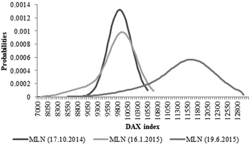
Table 3. Implied moments extracted from estimated implied probability distributions at three expiration dates based on MLN model for 1-month maturity horizon.

Implied moments	17.10.2014	16.01.2015	19.06.2015
µ	9851.40	9784.38	11446.08
σ	431.80	480.90	752.90
α3	1.39	–0.86	–0.60
α4	2.34	3.90	3.25

On third Friday in September, 2014 the value of DAX index was still recovering from its’ plunge in August. Therefore, the market sentiment was optimistic at 17 October 2014 yielding with higher expected value of DAX index one month ahead, lower volatility and positive skewness, i.e., market perceived the probability of positive outcomes to be higher than the probability of negative outcomes. Results for 16.01.2015 show similar implied mean but higher implied volatility with implied skewness concentrated on the left tail of the distribution. Moreover, as implied kurtosis is increasing a distribution has heavier tails. On 19.06.2015 the expected value of DAX was at higher level with higher implied volatility. Distribution is more negatively skewed on the left tail then on the right tail even both tails are heavier compared to other distributions, i.e., market participants perceive great uncertainty with the development of the DAX during the life of options with higher probability of negative outcomes, i.e., market sentiment was pessimistic.

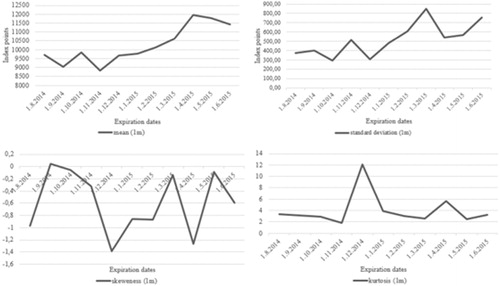
Figure 2 shows implied moments, mean, standard deviation, skewness and kurtosis, for all expiration dates using MLN model for 1-month maturity horizon. Expected and observed values of DAX index move along. Standard deviation increases as the expected value increases, indicating lower risk in the beginning and higher risk in the latter periods. This is in line with Aguilar and Hördahl (1999) who concluded that RNDs provide an indication of the market’s assessment concerning the uncertainty of future events, which vary substantially over time. Skewness is on average negative, indicating that market perceives the probability of negative outcomes to be higher than the probability of positive outcomes. Leptokurosis and fat-taildness are observed at the most expiration dates. This could be an indication of agitated periods since the results of Jackwerth and Rubinstein (1996) identify a distinct change in shape between the precrash (log-normal) and the postcrash distributions (leptokurtosis and left-skewness). Finally, extracted implied distribution reveals market sentiment, but it does not anticipate movements of DAX as was concluded in Gemmill and Saflekos (2000).

Figure 2. Implied moments at all expiration dates based on MLN model for 1-month maturity horizon.

5. Conclusion

In this article three non-structural approaches for estimation of implied probability distribution, i.e., mixture of two log-normals (MLN), Edgeworth expansion (EE) and Shimko’s model (SM), the representatives of parametric, semiparametric and nonparametric approaches respectively, are estimated and compared using one-year data for DAX index options, i.e., from July 2014 to July 2015. Non-structural models assume that only dynamics in prices is known. All three approaches have both advantages and disadvantages. However, previous researches reveal that none of the approaches is clearly superior to the others. Therefore, this research is conducted in order to compare the three selected models in their forecasting ability and within the models the focus is put on comparison regarding different maturity horizons. The results, valid for the selected period and for DAX index options, reveal that no matter which non-structural model is used they all give better short-term forecasts. In pairwise comparison for short-term prediction, MLN approach is superior according to the MSE and DM test. Moreover, MLN model is proven to be flexible, i.e., it is possible to obtain a wide variety of different implied probability distributions and it can capture commonly observed characteristics of financial assets, such as asymmetries and fat-tails in implied probability distributions. The results also reveal how the implied moments and implied probability distribution function itself respond to new information and how market assesses risk over time. Changes in the implied moments in observed period reveal that the value of DAX is at higher level with higher implied volatility and that implied probability distribution is more negatively skewed on the left tail then on the right tail. Implied probability distribution not only moves along with the index, but it also changes shape. Although the extracted implied probability distributions reveal market sentiment, they do not anticipate movements of DAX index. Since the values of true variance, skewness and kurtosis are unknown, i.e., cannot be observed, these implied moments can only be compared with their realised counterparts. That would be worth for further research which requires high frequency data. Different methods can be compared within different markets since they differ in liquidity. Therefore, development of option trading on emerging markets can be viewed as a new niche in modelling market expectations. Moreover, it would be interesting to verify the stability and validity of results for other markets and longer time series.

Disclosure statement

No potential conflict of interest was reported by the authors.

Additional information

Funding

This work has been fully supported by Croatian Science Foundation under the project “Volatility measurement, modelling and forecasting” (5199).

References

- Aguilar, J., & Hördahl, P. (1999). Option prices and market expectations. Sveriges Riksbank Quarterly Review, 1, 43–70.
- Andersen, A. B., & Wagener, T. (2002). Extracting risk neutral probability densities fitting implied volatility smiles: Some methodological points and an application to the 3M Euribor futures option prices (ECB Working Paper, No. 198). Retrieved from: http://ssrn.com/abstract=359060
- Aparicio, S. D., & Hodges, S. (1998). Implied risk-neutral distribution: A comparison of estimation methods. Retrieved from: http://www2.warwick.ac.uk/fac/soc/wbs/subjects/finance/research/wpaperseries/1998/98-95.pdf
- Arnerić, J., Aljinović, Z., & Poklepović, T. (2015). Extraction of market expectations from risk-neutral density. Zbornik Radova Ekonomskog Fakulteta u Rijeci :Časopis za Ekonomsku Teoriju/Proceedings of Rijeka Faculty of Economics:Journal of Economics and Business, 33(2), 235–256. doi: 10.18045/zbefri.2015.2.235
- Bahaludin, H., & Abdullah, M. H. (2017). Comparison of volatility function technique for risk-neutral densities estimation. Proceedings of the 24th National Symposium on Mathematical Sciences. AIP Conf. Proc. 1870, 040073-1–040073-8. doi: 10.1063/1.4995905
- Bahra, B. (1997). Implied risk-neutral probability density functions from option prices: Theory and application (Bank of England Working Paper, No. 66). Bank of England. doi: 10.2139/ssrn.77429
- Benavides, G., & Mora, I. F. (2008). Parametric vs. non-parametric methods for estimating option implied risk-neutral densities: The case of the exchange rate Mexican Peso – US Dollar and Mexican interest rates, Ensayos–Volumen, XXVII(1), 33–52.
- Black, F., & Scholes, M. S. (1973). The pricing of options and corporate liabilities. Journal of Political Economy, 81(3), 637–659. doi: 10.1086/260062
- Bliss, R. R., & Panigirtzoglou, N. (2002). Testing the stability of implied probability density functions. Journal of Banking and Finance, 26 (2-3), 381–422. doi: 10.1016/S0378-4266(01)00227-8
- Breeden, D. T., & Litzenberger, R. H. (1978). Prices of state-contigent claims implicit in option prices. The Journal of Business, 51(4), 621–651. doi: 10.1086/296025
- Breeden, D. T., & Litzenberger, R. H. (2014). Central Bank Policy Impacts on the Distribution of Future Interest Rates. SSRN Electronic Journal. doi: 10.2139/ssrn.2642363
- Cheng, K. C. (2010). A new framework to estimate the risk-neutral probability density functions embedded in option prices (IMF Working Paper, No. WP/10/181). International Monetary Fund. doi: 10.5089/9781455202157.001
- Christoffersen, P., Jacobs, K., & Chang, B. Y. (2012). Forecasting with option-implied information. In G. Elliott, & A. Timmermann (Eds.), Handbook of economic forecasting (Vol. 2). Available at https://ssrn.com/abstract=1969863 or http://dx.doi.org/10.2139/ssrn.1969863 [2.7.2018.].
- Coutant, S., Jondeau, E., & Rockinger, M. (2001). Reading PIBOR futures options' smile: The 1997 snap election. Journal of Banking and Finance, 25(11), 1957–1987. doi: 10.1016/S0378-4266(00)00161-8
- Datta, D. D., Londono, J. M., & Ross, L. J. (2017). Generating options-implied probability densities to understand oil market events. Energy Economics, 64(C), 440–457.
- Diebold, F. X., & Mariano, R. S. (1995). Comparing predictive accuracy. Journal of Business and Economic Statistics, 13(3), 253–263. doi: 10.3386/t0169
- Duca, I. A., & Ruxanda, G. (2013). A view on the risk-neutral density forecasting of the DAX30 returns. Romanian Journal of Economic Forecasting, 2, 101–114.
- Figlewski, S. (2009). Estimating the implied risk neutral density for the U.S. market Portfolio. In T. Bollerslev, J. R. Russell, & M. Watson (Eds.), Volatility and time series econometrics: Essays in honor of Robert F. Engle. Oxford: Oxford University Press. doi: 10.1093/acprof:oso/9780199549498.003.0015
- Flamouris, D., & Giamouridis, D. (2002). Estimating implied PDFs from American options on futures: A new semiparametric approach. Journal of Futures Markets, 22(1), 1–30.
- Gemmill, G., & Saflekos, A. (2000). How useful are implied distributions? Evidence from stock index options. The Journal of Derivatives, 7(3), 83–91. doi: 10.3905/jod.2000.319123
- Grith, M., & Krätschmer, V. (2011). Parametric modelling and estimation of risk-neutral densities. In J. C. Duan, J. E. Gentle, & W. Härdle (Eds.), Handbook of computational finance (pp. 253–275). Berlin, Heidelberg: Springer..
- Grith, M., Härdle, W. K., & Schienle, M. (2011). Nonparametric estimation of risk-neutral densities. In J. C. Duan, J. E. Gentle, & W. Härdle (Eds.), Handbook of computational finance (pp. 277–305). Berlin, Heidelberg: Springer.
- Jackwerth, J. C. (1999). Option implied risk-neutral distributions and implied binomial trees: A literature review. Journal of Derivatives, 7(2), 66–82.
- Jackwerth, J. C., & Rubinstein, M. (1996). Recovering probability distribution from option prices. The Journal of Finance, 51(5), 1611–1631.
- Jarrow, R., & Rudd, A. (1982). Approximate option valuation for arbitrary stochastic processes. Journal of Financial Economics, 10(3), 347–369. doi: 10.1016/0304-405x(82)90007-1
- Jondeau, E., Poon, S., & Rockinger, M. (2007). Financial modelling under non-Gaussian distributions. London: Springer-Verlag. doi: 10.1007/978-1-84628-696-4
- Jondeau, E., & Rockinger, M. (2000). Reading the smile: The message conveyed by methods which infer risk neutral densities. Journal of International Money and Finance, 19(6), 885–915.
- Khrapov, S. (2014). Option pricing via risk-neutral density forecasting. 2nd International Workshop on “Financial Markets and Nonlinear Dynamics” (FMND), June 4–5, 2015, Paris, France. Retrieved from: https://editorialexpress.com/cgi-bin/conference/download.cgi?db_name=SNDE2015&paper_id=110
- Liu, X., Shackleton, M. B., Taylor, S. J., & Xu, X. (2007). Closed-form transformations from risk-neutral to real-world distributions, Journal of Banking & Finance, 31(5), 1501–1520.
- Malz, A. M. (2014). A simple and reliable way to compute option-based risk-neutral distributions (Federal Reserve Bank of New York Staff Reports, No. 677). Federal Reserve Bank of New York. doi: 10.2139/ssrn.2449692
- Merton, R. C. (1973). Theory of rational option pricing. The Bell Journal of Economics and Management Science, 4(1), 141–183. doi: 10.1142/9789812701022_0008
- Mizrach, B. (2010). Estimating implied probabilities from option prices and the underlying. In C.-F. Lee, A. C. Lee, J. Lee (Eds), Handbook of quantitative finance and risk management (pp. 515–529). Berlin, Heidelberg: Springer. doi: 10.1007/978-0-387-77117-5_35
- Santos, A., & Guerra, J. (2015). Implied risk neutral densities from option prices: Hypergeometric, spline, lognormal, and edgeworth functions. Journal of Futures Markets, 35(7), 655–678. doi: 10.1002/fut.21668
- Shimko, D. (1993). Bounds of probability. Risk, 6, 33–37.
- Smith, T. (2012). Option-implied probability distributions for future inflation. Bank of England Quarterly Bulletin, Q3, 224–233. Available at http://ssrn.com/abstract=2150092.
- Söderlind, P. (2000). Market expectations in the UK before and after the ERM crisis. Economica, 67, 1–18. doi: 10.1111/1468-0335.00192
- Tavin, B. (2011). Implied distribution as a function of the volatility smile. Bankers Markets and Investors, 119, 31–42. doi: 10.2139/ssrn.1738965
- Vähämaa, S. (2005). Option-implied asymmetries in bond market expectations around monetary policy actions of the ECB. Journal of Economics and Business, 57(1), 23–38. doi: 10.1016/j.jeconbus.2004.07.003
- Xiao, X., & Zhou, C. (2017). Entropy-based implied moments (DNB Working Paper, No. 581). De Nederlandsche Bank, Amsterdam, The Netherlands.