Analysis of forecasts of GDP growth and inflation for the Croatian economy

Abstract

The paper provides, for the first time, the analysis of the quality of the GDP growth and inflation forecasts by multiple forecasters for the Croatian economy. Forecast data of 6 different institutions in the 2006–2015 period are analysed. Efficiency and biasedness test are conducted following the Davies and Lahiri econometric framework based on a three-dimensional panel dataset which includes multiple individual forecasters, target years and forecast horizons. In order to assess directional accuracy we follow the approach by Pesaran and Timmermann. Based on MAE values we find the forecasts to be accurate on a scale comparable to the European Commission’s forecast reported in 2016 for the EU and the euro area. GDP growth forecasts exhibit a strong bias related to a notable tendency to over-predict GDP growth. In the case of inflation forecasting the bias is still present for all forecasters, albeit less pronounced and not statistically significant for all of them. There is evidence of forecast inefficiency regarding both analysed variables. Overall, inflation forecasting presents less of a challenge due to specific monetary policy strategy and inaccurate national accounts data accompanied by extended revision process of the GDP data by the government’s statistics office.

Keywords:

• GDP growth rate
• inflation
• forecasting
• three-dimensional panel

JEL CLASSIFICATIONS:

• C53
• E37
• P2

1. Introduction

Forecasts of key macroeconomic variables are important to all economic agents. However, forecasting is essential for government institutions (central banks, treasury departments or ministries and other government bodies) and international economic organisations such as the International Monetary Fund (IMF), the World Bank (WB), the Organisation for Economic Co-operation and Development (OECD), the European Bank for Reconstruction and Development (EBRD) and others.

Although the European Commission’s (EC) forecasts have already been assessed twice and regardless of the fact that the EC has monitored Croatia’s macroeconomic development ever since it was officially granted its European Union (EU) candidate country status in 2004, Croatia has been left out of the recent study due to insufficient data. Thus, to the best of the authors’ knowledge, the research by Krkoska and Teksoz (2007) remains the only analysis of forecast accuracy to include data regarding Croatian economy. However, the research was based on EBRD’s GDP growth forecasts and included 25 transition countries from central and eastern Europe and former Soviet Republics with the results only being reported at the aggregate level (for the whole sample and three sub-regions the countries were grouped into).

Therefore, since for Croatia forecast accuracy results have never been reported in detail, irrespective of the institution providing the forecasts or the variables being forecasted, our paper aims to provide such an analysis. The analysis we conducted focuses on the forecasts of the real GDP growth rate and inflation by applying the econometric framework originally developed by Davies and Lahiri (1995) for the purposes of biasedness and efficiency assessment. Directional accuracy tests follow the work of Pesaran and Timmermann (1992) allowing the results to be comparable to the EC’s study by Fioramanti, Gonzales Cabanillas, Roelstraete, and Ferrandis Vallterra (2016).

Furthermore, according to Sosvilla-Rivero and Ramos-Herrera (2018), studies on alternatives to rational expectations assumptions cannot develop on their own, as empirical research is needed to channel the efforts. Thus, empirical research in this paper provides foundation for future research efforts regarding not only Croatian economy but even more generally. Namely, as findings across countries differ in many respects and as at the moment there is no way of knowing how forecasts for Croatian economy behave in any of the ways typically analysed, assessment in this paper sheds light on some of the key aspects for this small and open economy characterised also by the EU integration processes. The interpretation of results in relation to other empirical research findings analysed reveals possible factors that affect similarities and differences between countries. In this regard it should be noted in particular that the analysis is being conducted for the EU member state that was hardest hit by the 2008 financial crisis (fall in real GDP for 6 consecutive years, 2009–2014). This is interesting from the perspective stressed by IMF (2018) as forecasts for low-income countries are identified as the main drivers of forecast bias and inefficiency which could be related to larger shocks and lower data quality associated to those economies. Even though Croatia is not a low-income country from the IMF’s, i.e. global, perspective, it could be viewed as such from the EU’s perspective.

The rest of the paper is organised as follows. Section 2 presents the literature review. Section 3 describes the data and provides the initial analysis. The econometric framework used for further analysis is described in Section 4. The results of the empirical research are presented in Section 5. Finally, Section 6 provides the main findings and conclusions that have been reached.

2. Literature review

In 2000s the research on forecast accuracy for the developed economies based on the methodological framework developed in the 1990s was published. Notable papers include the research by Öller and Barot (2000) who analysed forecasts of Gross Domestic Product (GDP) growth and inflation by OECD and national institutes for 13 European countries, Boero, Smith, and Wallis (2008) who analysed the same for the UK economy and Clements, Joutz, and Stekler (2007) who analysed forecasts of GDP growth, inflation and unemployment for the US economy. In their analysis, Öller and Barot (2000) test forecast accuracy, biasedness and efficiency, while Clements et al. (2007) and Boero et al. (2008) focus on biasedness and efficiency by introducing the pooled data (three-dimensional panel) approach as proposed originally by Davies and Lahiri (1995).

Therefore, in the last decade, research papers and reports emerged combining the above approaches as standard practice in order to assess an institution’s forecasts, often written by the institution’s own staff or experts working in association with them. Examples include research by Krkoska and Teksoz (2007) for EBRD’s forecasts, Cabanillas and Terzi (2012) and Fioramanti et al. (2016) for European Commission’s forecasts and evaluation reports on their own forecasts by the IMF (2014) and the Bank of England (2015).

However, forecast analysis of macroeconomic variables still remains a dynamic field of research covering different regions of the world dealing with efforts to improve overall forecasting abilities while also trying to capture different country-specific issues. For instance, Chen, Costantini, and Deschamps (2016) analyse the accuracy of GDP growth and inflation forecasts in Asia, while Pierdzioch and Rülke (2015) focus on exchange rate forecasts in emerging economies in Asia, eastern Europe and South America. When it comes to single economy study, Tsuchiya and Suehara (2015) and Deschamps and Bianchi (2012) focus on China, Carvalho and Minella (2012) and Baghestani and Marchon (2015) deal with Brazil, Capistran and Lopez-Moctezuma (2014) investigate Mexican inflation and GDP growth forecasts, while Baghestani and Danila (2014) focus on inflation forecasting in the Czech Republic.

Although the above mentioned research sometimes differs in approaches and methods used, inflation and real growth rate of GDP dominate as macroeconomic variables analysed. Moreover, the three research papers that analyse both inflation and real GDP growth rates, Deschamps and Bianchi (2012), Capistran and Lopez-Moctezuma (2014) and Chen et al. (2016) all use the three-dimensional panel of forecasts to test biasedness and efficiency. Forecast accuracy evaluation differs in approaches when it comes to directional accuracy testing with some researchers omitting this specific assessment such as Deschamps and Bianchi (2012) and Capistran and Lopez-Moctezuma (2014). Research findings vary as they depend on the forecaster, variable, country, time horizon of the forecasts and even on the economic cycle according to Deschamps and Bianchi (2012) and IMF (2018). However, forecasts do seem to exhibit, as would be reasonable to expect, a general tendency of improving as forecast horizons become shorter. Some authors, most notably Boero et al. (2008), Capistran and Lopez-Moctezuma (2014) and Chen et al. (2016) relate this to slow adjustments of forecasters’ expectations implying an asymmetric loss function leading to increased forecast error. Therefore, research efforts are devoted to this particular problem alone such as in Behrens, Pierdzioch, and Risse (2018) who use random forests method developed in the machine-learning literature to analyse whether forecasters have flexible rather than symmetric (quadratic) loss function.

3. Data structure and initial analysis

The forecast data are collected (only as point forecasts¹) in the period from 2006 to 2015 for 6 institutions which have continuously produced forecasts² regarding inflation and real growth rate of GDP for Croatia, albeit, understandably, at different frequencies and points in time. Thus, some of the forecast horizons in the collected data set were left with fewer data and fewer contributors and were therefore not included in the analysis. The number of forecast data per institution and horizon is presented in Tables 1 and 2 regarding the GDP growth and inflation respectively.

Table 1. The number of available forecast data for the real growth rate of GDP (horizon in months).

Institution\Horizon	3	6	9	12	15	18	21	24	27	30	Total
1	4	10		10	3	10		10	2	10	59
2	8	9	9	9	9	8	8	7	6		73
3	10	10	9	8	9	9	8	7	8	7	85
4	10	10	9	9	9	9	8	8	8	7	87
5		10		10		9		9		6	44
6	8		8		8		4		2		30
Total	40	49	35	46	38	45	28	41	26	30	378

Table 2. The number of available forecast data for inflation (horizon in months).

Institution\Horizon	3	6	9	12	15	18	21	24	27	30	Total
1	3	9	1	10	2	10		10	2	10	57
2	10	8	8	9	9	8	8	8	6		74
3	10	10	9	8	9	9	8	7	8	7	85
4	9	10	9	9	9	9	8	8	8	7	86
5		10		10		9		9		6	44
6	6		5		5		4		2		22
Total	38	47	32	46	34	45	28	42	26	30	368

Regarding both the GDP growth rate and inflation, forecast horizons 21, 27 and 30 months ahead were filtered out due to having 30 or less forecasts in total and mostly only four contributing institutions out of six. This also explains why adding more forecasters to the analysis is not easy. The institutions chosen for the purposes of this research have a lot of matching forecast horizons (the only notable exception being institutions 5 and 6 whose mutual horizons do not match at all) which helps with econometric tests and the interpretation of results. Furthermore, it should be mentioned that for the purpose of conducting econometric tests in the fifth section of the paper, further forecast horizons (containing 4 or less forecasts) had to be eliminated for the institution number 1 for both variables analysed.³ This, also implies that institution number 6 barely met the inclusion criteria regarding the available forecast data for inflation.

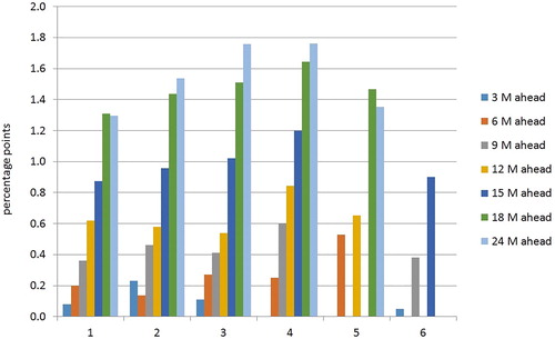
The group of six forecasting institutions consists of two international institutions and four domestic ones out of which two are privately owned financial institutions and the others are from the public sector. The initial analysis of collected data in terms of simple MAE (Mean Absolute Error) generally shows a rising trend in forecast error as the forecast horizon gets longer (for both inflation and GDP growth rate) as expected. This is presented in Figures 1 and 2.

Figure 1. Average MAE per institution and horizon for the GDP growth.

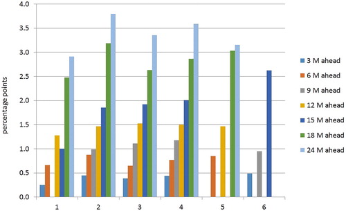
Figure 2. Average MAE per institution and horizon for inflation.

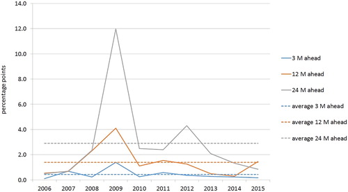
Also using MAE, the average forecast error for all institutions can be tracked over the analysed period for each forecast horizon. Figure 3 for the GDP growth rate shows again the growing forecast error as the forecast horizon gets longer but also shows the significant influence of financial crisis with the biggest forecast error in the year 2009 across forecast horizons.⁴ A smaller rise in forecast errors is also present in the year 2012 as a fall in GDP declined from −7.4% and −1.7% in 2009 and 2010 to −0,3% in 2011 inducing optimism which later turned out to be unsubstantiated as the new government took office in 2012. Only 3 forecast horizons (the shortest, the longest and the middle one) are reported as the average MAE for all other horizons exhibit similar behaviour that falls in between of what is presented here.

Figure 3. Average MAE for the GDP growth per selected forecast horizons.

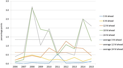
Figure 4, which shows the average MAE for inflation for all institutions per different forecast horizons, shows lower MAE values suggesting that forecasters were much better at forecasting inflation than GDP growth.⁵ However, the patterns of deviations from average are in this case more difficult to interpret as occasional spikes vary from horizon to horizon. It can be noted however that financial crisis did play a role here also but only in the case of forecast horizons of 18 and 24 months (which generally exhibit more frequent deviations from the average values). Also, a significant rise in MAE for the same horizons is present in the 2014 and 2015 which can most likely be attributed to a rise in inflation in 2011-2013 (both in Croatia and the euro area) and expectations of GDP growth.

Figure 4. Average MAE for inflation per selected forecast horizons.

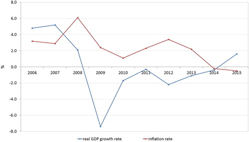
The actual values of the inflation and real growth rate of GDP are shown in Figure 5 but it should be pointed out that values for GDP in 2014 and 2015 are yet only estimates of the Croatian Bureau of Statistics.

Figure 5. The actual values of the real growth rate and inflation.

Source: Croatian Bureau of Statistics.

Further analysis based on the data presented above is described in the fifth section, which contains research findings.

4. The econometric framework

The data are described and analysed as a three-dimensional panel with multiple individual forecasters, target years, and forecast horizons. To analyse such collection of expectations of future inflation and GDP growth values and give insights into the quality of the forecasts, we use the framework first developed by Davies and Lahiri (1995) and expanded further by Davies and Lahiri (1999), Davies (2006) and Davies, Lahiri, and Sheng (2011). The framework can be used to test the rational expectations hypothesis correctly.

We adopt the notational convention of the mentioned Davies-Lahiri framework and denote as F_ith the forecast for target period t, made by individual i, h periods prior to the end of period t (i.e. prior to the realization of the target). The actual outcome for the variable of interest at the end of period t is denoted as A_t. The correct way to decompose the forecast error suggested by the framework is: (1) $$A_t-F_{\mathit{ith}}={\lambda }_{th}-{\varphi }_{ih}-{\epsilon }_{\mathit{ith}},$$(1) where i = 1,…, N, t = 1,…, T, h = 1,…, H.

Equation (1)(1) $$A_t-F_{\mathit{ith}}={\lambda }_{th}-{\varphi }_{ih}-{\epsilon }_{\mathit{ith}},$$(1) identifies three components of the forecast error: cumulative shocks λ_th which represent the cumulative effect on A_t of uncorrelated period-by-period aggregate unforecastable shocks that occurred between the time at which the forecast was made and the time at which the actual was realized; the forecasters’ bias ϕ_ih which is a possible systematic effect that varies according to the individual forecasting and to the horizon at which the individual stands; and ε_ith as an idiosyncratic non-autocorrelated error and deviations in the forecaster’s information set from the publicly available information set. General expressions for estimates of the forecast error components are: (2) $${-\widehat{\varphi }}_{ih}=\frac{1}{T}\sum _{t=1}^T\left(A_t-F_{\mathit{ith}}\right)$$(2) $${\widehat{\lambda }}_{th}=\frac{1}{N}\sum _{i=1}^N\left(A_t-F_{\mathit{ith}}+{\widehat{\varphi }}_{ih}\right)$$ $${\widehat{\epsilon }}_{\mathit{ith}}={-A}_t+F_{\mathit{ith}}-{\widehat{\lambda }}_{th}+{\widehat{\varphi }}_{ih}$$

The framework develops special expressions for the NTH × NTH forecast error covariance matrix Σ to take care of the substantial covariance between individual errors due to aggregate shocks. After calculating matrix Σ, the general method of moments estimation is employed and the standard errors for the bias are obtained as the square roots of the diagonal of (X´X)⁻¹X´ΣX(X´X)⁻¹, where X is an NTH × NTH matrix of individual- and horizon-specific dummies.

If a common bias across horizons is assumed, i.e. if biases are restricted to be individual specific only, the restrictions ϕ_ih=ϕ_i, ∀h need to be imposed and the general method of moments tests should be re-ran. The expression for individual-specific bias is: (3) $${-\widehat{\varphi }}_i=\frac{1}{TH}\sum _{t=1}^T\sum _{h=1}^H\left(A_t-F_{\mathit{ith}}\right).$$(3)

To test efficiency we check for a correlation between the forecast error and information that was known to the forecaster at the time the forecast was made. Within the framework the correct expression for the efficiency test is: (4) $$A_t-F_{\mathit{ith}}=\delta X_{t,\mathrm{ }h+1}+{\lambda }_{th}-{\varphi }_{ih}-{\epsilon }_{\mathit{ith}},$$(4) where X_t,h+1 is information known to the forecaster at the time the forecast was made. The hypothesis of efficiency is rejected if $\widehat{\delta }$≠0. Although some authors (Davies & Lahiri, 1999; Clements et al., 2007) recommend applying GMM to the first-difference transformation of equation (4)(4) $$A_t-F_{\mathit{ith}}=\delta X_{t,\mathrm{ }h+1}+{\lambda }_{th}-{\varphi }_{ih}-{\epsilon }_{\mathit{ith}},$$(4) , we do not pursue this possibility due to problems with the structure of our dataset, available horizons and missing data. Thus, we simply perform regression of the forecast errors on the variables that are likely members of the information set, as for example in Boero et al. (2008).

Since rationality requires both unbiasedness and efficiency, a forecaster who fails either is considered irrational. Along with the rationality tests, we give the forecasts evaluations in terms of their root mean square error (RMSE) and mean absolute error (MAE). Moreover, in order to examine whether the forecasts predict the sign of the outcome i.e., whether the forecasts and the actual outcome move in the same direction (increase versus decrease, growth versus recession, inflation versus deflation), we perform directional accuracy test implemented by Pesaran and Timmermann (1992). It is a distribution-free procedure for testing the accuracy of forecasts focusing on the prediction of the direction of change in the variable under consideration. We performed the test using DACTest function from rugarch package of R (Ghalanos, 2014, R Core Team, 2013) and since this represents the test in its original form presented in Pesaran and Timmermann (1992) we omit the formulas and refer the reader to the references above in order to remain concise. Also, we perform a more stringent test in this regard to check whether acceleration (pick-up) and deceleration (slowdown) in the economy can be forecasted. A pick-up in GDP growth (inflation) means that the difference between GDP growth (inflation) in year t and year t-1 is positive, while a slowdown means the opposite effect. For the change in forecasts for year t, the difference between forecasts separated by one year is used. To investigate whether a pick-up or a slowdown has been predicted accurately, the data are here again analysed using the Pesaran and Timmermann test (1992).

5. Results

5.1. Forecast absolute errors, root mean squared errors and directional accuracy

Tables 3 and 4 report RMSE and MAE, as well as directional accuracy test results for GDP growth and inflation forecasts respectively. It should be noted that for some forecasters at certain horizons GDP growth and inflation forecasts are always positive, which means that the Pesaran-Timmermann directional accuracy test relating to increase/decrease in the value cannot be performed (NA). Moreover, there are two cases of forecasting acceleration of GDP growth for all years, which also makes the Pesaran-Timmermann test impossible to perform. On the other hand, there is no such problem with the accuracy test regarding the acceleration/deceleration of inflation. Also, since the change in forecasts for year t is calculated as the difference between forecasts separated by one year (12 months), acceleration/deceleration accuracy tests cannot be performed for horizons less than 15 months.

Table 3. RMSE, MAE and directional accuracy of GDP growth forecasts.

Forecaster	Horizon	MAE	RMSE	Accuracy (increase/decrease)	Accuracy (acceleration/deceleration)
1	24	2.910	4.452	NA	0.778*
1	18	2.480	3.707	0.400	0.889***
1	12	1.280	1.777	0.900***
1	6	0.660	0.816	0.900***
2	24	3.800	5.199	NA	NA
2	18	3.188	4.432	NA	0.875**
2	15	1.856	2.459	0.778**	0.857**
2	12	1.467	1.906	0.889***
2	9	0.989	1.349	0.889***
2	6	0.878	1.083	0.889***
2	3	0.450	0.652	0.875***
3	24	3.357	4.890	NA	0.714*
3	18	2.633	3.953	0.444	0.667
3	15	1.922	2.418	0.667	0.778**
3	12	1.525	1.848	0.750*
3	9	1.111	1.332	0.889***
3	6	0.650	0.774	0.900***
3	3	0.390	0.538	0.900***
4	24	3.588	4.995	NA	NA
4	18	2.867	3.846	0.222	0.039
4	15	2.011	2.713	0.556	0.889***
4	12	1.500	1.863	0.778*
4	9	1.178	1.455	0.889***
4	6	0.770	0.941	0.900***
4	3	0.440	0.593	0.900***
5	24	3.151	4.378	NA	0.889***
5	18	3.035	4.268	NA	0.889***
5	12	1.462	1.771	0.800**
5	6	0.851	1.050	0.900***
6	15	2.625	3.457	0.375	1.000***
6	9	0.950	1.236	0.875**
6	3	0.488	0.625	0.875**

Significance at the 10%, 5% and 1% levels is indicated by single, double and triple asterisks, respectively. NA means that the test cannot be performed because all forecasts are positive.

Table 4. RMSE, MAE and directional accuracy of inflation forecasts.

Forecaster	Horizon	MAE	RMSE	Accuracy (increase/decrease)	Accuracy (acceleration/deceleration)
1	24	1.294	1.522	NA	0.556
1	18	1.310	1.564	NA	0.667
1	12	0.619	0.820	1.000***
1	6	0.201	0.291	NA
2	24	1.538	1.871	NA	0.500
2	18	1.438	1.713	NA	0.875***
2	15	0.956	1.430	0.667	0.778*
2	12	0.578	0.632	NA
2	9	0.463	0.483	NA
2	6	0.138	0.162	1.000***
2	3	0.230	0.667	1.000***
3	24	1.757	2.080	NA	0.857**
3	18	1.511	1.832	NA	0.667*
3	15	1.022	1.294	NA	0.667*
3	12	0.538	0.677	0.750
3	9	0.411	0.482	0.778
3	6	0.270	0.315	0.900**
3	3	0.110	0.130	0.900**
4	24	1.763	2.081	NA	0.625*
4	18	1.644	1.911	NA	0.667*
4	15	1.200	1.308	NA	0.625*
4	12	0.844	0.939	NA
4	9	0.600	0.629	0.778
4	6	0.250	0.292	0.800
4	3	0.000	0.000	1.000***
5	24	1.353	1.664	NA	0.556
5	18	1.466	1.809	NA	0.556
5	12	0.653	0.794	0.900**
5	6	0.530	0.601	1.000***
6	15	0.900	0.999	NA	0.600
6	9	0.380	0.397	0.600
6	3	0.050	0.071	1.000***

Significance at the 10%, 5% and 1% levels is indicated by single, double and triple asterisks, respectively. NA means that the test cannot be performed because all forecasts are positive.

The analysis of GDP growth data shows that the performance of the forecasters varies widely considering the MAE and RMSE results, especially for shorter forecasting horizons. At the shortest horizon, i.e. 3 months, the best forecaster in the panel has a MAE of 0.390 compared to the worst forecaster whose MAE is 0.488, while RMSE lies in the range of 0.538 and 0.652. At the longest horizon, i.e. 24 months, the best forecaster in the panel has a MAE of 2.910 compared to the worst forecaster whose MAE is 3.800, while RMSE values are in the range of 4.378 and 5.199. Also, as expected, MAE and RMSE tend to be larger as the forecasting horizon increases as less information is available at the time of forecasting. Nevertheless, most of these errors in GDP growth seem quite large but can be attributed to a relatively volatile period of GDP growth in which the actual GDP growth ranged between -7.4 and 5.2 as discussed further later in this section. However, the directional accuracy test results reveal that all forecasters are successful in predicting the sign of GDP at horizons 12 and less. Forecaster 2 also successfully predicted the sign of GDP at horizon 15. Moreover, they are found to be predicting pick-ups and slowdowns in GDP successfully for certain horizons. For example, even for horizon of 24 months, forecaster 5 correctly predicted if there will be a pick-up or a slowdown in 88.9% of the cases.

Inflation data analysed in Table 4 exhibits less variation in MAE and RMSE values. At the shortest horizon, i.e. 3 months, the best forecaster in the panel has a MAE of 0 compared to the worst forecaster whose MAE is 0.230, while RMSE lies in the range of 0 and 0.667. At the longest horizon i.e. 24 months, the best forecaster in the panel has a MAE of 1.294 compared to the worst forecaster whose MAE is 1.763, while RMSE values are in the range of 1.522 and 2.081. The actual inflation ranged between -0.5 and 6.1. In the case of inflation it is even more obvious that MAE and RMSE tend to be larger as the forecasting horizon increases (as already mentioned in the third section of the paper and presented in the Figure 2). Looking at the directional accuracy test results, all forecasters seem successful in predicting the sign of inflation for some horizons, albeit, mostly shorter ones. However, those results could be misleading when judging inflation forecasts quality since the actual inflation was positive for most of the years in the sample. Thus, analysing pick-ups and slowdowns gives a better picture on directional accuracy. It can be noticed that only two forecasters (for one horizon each) managed to correctly predict inflation pick-ups and slowdowns at 5 per cent (or lower) level of significance.

5.2. Forecast bias end efficiency

Tables 5 and 6 contain the results of calculating the individual- and horizon-specific bias, as well as testing the efficiency of the forecasts, for GDP growth and inflation forecasts respectively.

Table 5. Bias and efficiency test results for GDP growth forecasts.

Forecaster	Horizon	${\widehat{\mathit{\varphi }}}_{\mathit{ih}}$	s.e.	$\widehat{\mathit{\delta }}$	s.e.
1	24	−2.490	0.270***
1	18	−1.920	0.183***	−0.740	0.588
1	12	−0.820	0.140***	−0.236	0.285
1	6	−0.420	0.233	−0.009	0.095
2	24	−3.543	0.338***
2	18	−2.838	0.199***	−2.667	0.420***
2	15	−1.389	0.181***	−0.928	0.328**
2	12	−1.022	0.126***	0.110	0.282
2	9	−0.700	0.107***	−0.028	0.181
2	6	−0.589	0.321	−0.017	0.115
2	3	−0.425	0.187*	0.064	0.057
3	24	−3.186	0.361***
3	18	−1.833	0.211***	−1.872	0.704**
3	15	−1.167	0.189***	−0.414	0.353
3	12	−0.675	0.179***	0.048	0.323
3	9	−0.578	0.119***	0.038	0.197
3	6	−0.250	0.244	−0.023	0.097
3	3	−0.250	0.159	0.072	0.045
4	24	−3.438	0.318***
4	18	−2.244	0.185***	−1.535	0.518**
4	15	−1.433	0.180***	−0.435	0.507
4	12	−0.833	0.132***	0.042	0.303
4	9	−0.844	0.103***	0.036	0.188
4	6	−0.410	0.282	0.045	0.114
4	3	−0.300	0.171	0.061	0.054
5	24	−2.729	0.648***
5	18	−2.680	0.504***	−0.694	0.739
5	12	−0.949	0.353***	−0.255	0.330
5	6	−0.569	0.294	0.073	0.123
6	15	−2.275	0.530***
6	9	−0.675	0.336**	−0.468	0.187**
6	3	−0.463	0.159**	0.041	0.063

Significance at the 10%, 5% and 1% levels is indicated by single, double and triple asterisks, respectively.

Table 6. Bias and efficiency test results for inflation forecasts.

Forecaster	Horizon	${\widehat{\mathit{\varphi }}}_{\mathit{ih}}$	s.e.	$\widehat{\mathit{\delta }}$	s.e.
1	24	−0.358	0.275
1	18	−0.278	0.200	0.134	0.722
1	12	−0.129	0.166	−0.339	0.242
1	6	−0.137	0.091	−0.138	0.042**
2	24	−0.513	0.303*
2	18	−0.363	0.206*	0.660	1.381
2	15	0.156	0.249	0.359	0.813
2	12	−0.200	0.150	0.056	0.151
2	9	−0.313	0.201	−0.021	0.119
2	6	−0.038	0.060	−0.028	0.035
2	3	0.190	0.213	−0.031	0.162
3	24	−0.586	0.317*
3	18	−0.511	0.194***	−0.095	1.955
3	15	−0.911	0.216***	−0.195	0.400
3	12	−0.438	0.151***	0.125	0.134
3	9	−0.300	0.140**	0.045	0.083
3	6	−0.110	0.098	−0.037	0.066
3	3	−0.090	0.031**	−0.003	0.018
4	24	−1.038	0.304***
4	18	−0.822	0.195***	0.567	1.464
4	15	−0.644	0.217***	−0.223	0.612
4	12	−0.378	0.152**	0.127	0.273
4	9	−0.422	0.141***	−0.032	0.123
4	6	−0.170	0.079*	0.007	0.051
4	3	0.000	NA	NA	NA
5	24	−0.309	0.286
5	18	−0.488	0.198**	−0.137	1.097
5	12	−0.184	0.145	−0.163	0.267
5	6	−0.302	0.173	−0.149	0.099
6	15	−0.460	0.298
6	9	−0.300	0.184	0.053	0.141
6	3	−0.050	0.022	−0.006	0.020

Significance at the 10%, 5% and 1% levels is indicated by single, double and triple asterisks, respectively. NA means that the test cannot be performed because all forecast errors are zero.

Having in mind the structure of the collected forecasts it should be noted that calculation of biases, within the Davies-Lahiri framework, required dividing the data into two groups. One group is comprised of the forecasters that forecast 6, 12, 18 and 24 months ahead and the other of those that forecast 3, 9 and 15 months ahead. For all horizons greater than 6 months, the individual- and horizon-specific bias ${\widehat{\varphi }}_{ih}$ is calculated as in Equation (2)(2) $${-\widehat{\varphi }}_{ih}=\frac{1}{T}\sum _{t=1}^T\left(A_t-F_{\mathit{ith}}\right)$$(2) , and standard error (s.e.) is calculated from the appropriate covariance matrix as explained in the previous section. The shortest horizons are lost due to missing data caused by differencing required within the Davies-Lahiri framework. Therefore, although utilising all the forecasts in a single test (i.e. pooling the forecasts for each variable across all horizons as in Davies-Lahiri framework) would make the test more powerful, in order to get some insight into the biases at smallest horizons, (the horizons of 3 and 6 months ahead) standard regression analysis had to be applied. Thus, we regress forecast errors on a constant and test whether the coefficient on the constant is significantly different from zero. To account for the small sample size, this regression is complemented by a Wilcoxon signed rank test with a null hypothesis that the median of the estimate of the variable of interest is equal to zero.

As explained in the previous section, the efficiency of the forecasts is tested by running the regression of the forecast error on the variables that were a part of the information set available at the time the forecast was made (Equation (4)(4) $$A_t-F_{\mathit{ith}}=\delta X_{t,\mathrm{ }h+1}+{\lambda }_{th}-{\varphi }_{ih}-{\epsilon }_{\mathit{ith}},$$(4) ). For the GDP growth forecasts, we perform this test using the following proxies for X_t,h+1:

1. forecast ahead, i.e. forecasters’ most recent GDP growth forecast,

2. GDP growth rate lagged three years which (most often) presents the latest available official final value of GDP growth rate,

3. estimated GDP growth rate lagged one year, i.e. latest available official estimation of actual value of GDP growth.⁶

However, in Table 5 only the results for regressing the error on the forecast ahead are reported since the two other variables are not significant for any forecaster at any horizon, at the usual levels of significance.

For inflation forecasts, the variables X_t,h+1 used for performing the efficiency tests are:

1. forecast ahead, i.e. forecasters’ most recent inflation forecast,

2. latest available actual value, i.e. inflation lagged one year.

In this case also only the results for regressing the error on the forecast ahead are reported in Table 6. When considering inflation lagged one year, we find significant regression results (at 10 per cent level, $\widehat{\delta }$=−0.396, s.e. =0.202) and hence a rejection of efficiency only in the case of forecaster 4 at horizon 12 of months ahead.

For GDP forecasts, the individual- and horizon-specific bias is negative for all forecasters at all horizons indicating a strong general tendency to over-predict GDP growth. At horizons from 24 down to 9 months ahead it is significantly different from zero at the 1 per cent level for all forecasters that forecasted at those horizons. It is reasonable to expect a reduction in the bias as the horizon declines and analysis of the GDP data does reveal a general trend of such a decline. However, most of the forecasters exhibit significant bias even at shorter horizons. In order to evaluate individual-specific bias only, i.e. assuming a common bias across horizons, we calculate biases by using Equation (3)(3) $${-\widehat{\varphi }}_i=\frac{1}{TH}\sum _{t=1}^T\sum _{h=1}^H\left(A_t-F_{\mathit{ith}}\right).$$(3) , as explained in the previous section. The results show that all forecasters have significant overall bias at 1 per cent level. Regarding efficiency, the results show that for three forecasters, the forecasts error at horizon of 18 months is predictable from the forecasts at horizon of 24 months, leading to the rejection of efficiency. Also, for one forecaster the forecasts error at horizon of 15 months is predictable from the forecasts at horizon of 18 months, and for one forecaster the forecasts error at horizon of 9 months is predictable from the forecasts at horizon of 15 months, therefore rejecting efficiency in these cases too. Since rationality requires both unbiasedness and efficiency, a forecaster who fails either is considered irrational. At the horizon of 6 months, forecasters 1, 2, 3, 4 and 5 pass this test, at all usual levels of significance. At the horizon of 3 months, forecasters 3 and 4 pass this test, at all usual levels of significance. In all the other cases the examined forecasters failed this rationality test for GDP growth forecasts. However, it is important to remember that the shortest horizons (3 and 6) are lost due to missing data caused by differencing required within the Davies-Lahiri framework as explained before. Therefore, weaker tests were used for biases for those shortest horizons, which should be taken into account when observing the sudden loss in bias significance in those cases.

The results for inflation forecast errors seem to show a less pronounced tendency towards over-prediction than the GDP forecast errors but still with negative bias for all of the respondents at all horizons, with just two notable exceptions. The first one is related to forecaster 4, who managed to predict inflation correctly and with forecast error equal to zero for all years at horizon of 3 months ahead, and the second one to forecaster 2, also at 3 months horizon. However, forecaster 4 exhibits significant biases at all other horizons, while on the other hand, for example, forecasters 1 and 6 do not show statistically significant bias at any horizon, at the usual levels of significance. Nevertheless, for forecaster 1, the forecast error at horizon of 6 months is predictable from the forecasts at horizon of 12 months, which leads to rejection of efficiency and hence rationality in this case. Regardless of deficiencies, the results suggest that the panel under study performs better in forecasting inflation than GDP growth since all of the forecasters managed to be rational at least at one of the analysed horizons.

5.3. Comments on the findings and comparison to similar studies

Regarding directional accuracy, Fioramanti et al. (2016), report MAE values for European Commission’s forecasts regarding GDP and inflation of EU member states, the EU and the euro area. For the GDP growth rate MAE for the EU stood at 0.48 and 0.92 while MAE for the euro area stood at 0.37 and 0.95 for the current year and 1 year ahead forecasts respectively. Also, based on the reported results we calculated⁷ the average MAE for all EU member states which stands at 1.069 for the current year forecast and 2.007 for the year-ahead forecast. For EU member states such as France, Austria, Belgium, the Netherlands and Germany MAE values were in the range of 0.54 and 0.78 for the current year forecasts and in the range of 0.84 and 1.25 for the year-ahead forecast. However, average forecast MAE for Latvia of 3.02 and Estonia of 2.52 were reported regarding current year forecast. Regarding average MAE for the year-ahead forecasts Estonia, Latvia and Lithuania stand out with MAE values of 4.18, 4.54 and 3.18 respectively. Similarly, Krkoska and Teksoz (2007) report average MAE of 3.15 for the year-ahead forecast horizon regarding EBRD’s forecasts of GDP growth rates for the south-eastern Europe transition countries. In the case of the central eastern Europe and the Baltic states the average MAE was 1.90. As can be seen from Table 3, the highest value of MAE of individual forecaster for Croatian economy stands at 0.488, 0.878 and 1.525 for the forecast horizons of 3, 6 and 12 months ahead respectively. Corresponding average MAE values on aggregate level (average of all forecasters) are 0.427, 0.751 and 1.385 for the forecast horizons of 3, 6 and 12 months ahead respectively.⁸ Therefore, it can be concluded that the results for the Croatian economy correspond to European Commission’s forecasts for the developed EU and euro area member states regarding MAE values for the current year GDP forecasts. Nevertheless, regarding the year-ahead forecasts, the results do seem to be slightly worse but still better than in the case of EBRD’s forecasts for the central eastern Europe and the Baltic states not to mention the south-eastern Europe transition countries.⁹

This somewhat surprising find can perhaps be explained by the fact that Croatia is a small and specific economy in case of which tourism and government spending for instance could have a more significant role in GDP growth forecasting than in other above mentioned countries. Such line of reasoning is to some extent backed up by Krkoska and Teksoz (2007, p. 42) who noted well, that for Croatia better forecast accuracy late within a year can be achieved as the impact of summer tourism season is known by then. However, in order to fully verify the postulated hypothesis, it would be necessary to pursue the research presented in IMF (2018) as it demonstrated a way to decompose forecast errors into sources and finding evidence that private consumption growth is the key contributor to GDP growth forecast error.

Regarding inflation, Fioramanti et al. (2016), reported MAE values for the EU of 0.3 and 0.8 and of 0.22 and 0.56 for the euro area for the current year and 1 year ahead forecasts respectively. However, based on the reported results an average MAE for all euro area member states was calculated standing at 0.69 for the current year forecast and 1.22 for the year-ahead forecast. As can be seen from Table 4 and Figure 4 the results for Croatian economy show low MAE values for Croatian economy (average for all forecasters of 0.098, 0.283 and 0.634 for horizons of 3, 6 and 12 months respectively)¹⁰ suggesting that forecasting inflation does not present a challenging task for the Croatian economy (especially compared to forecasting GDP growth rate).We argue that explanation is related to specific monetary policy framework in place in Croatia which is discussed in detail a little later.

Furthermore, regarding prediction of pick-ups and slowdowns, Fioramanti et al. (2016) report successful prediction in pick-ups and slowdowns on aggregate level (for all EU member states) in more than 80% of the cases for the current year for both inflation and GDP. The rates are lower for the year-ahead forecasts but never below 60%. Accuracy is found to be significant at 1% level of significance with just one exception in which case the level of significance is 5%. From Tables 3 and 4 it is obvious that results for Croatian economy are worse. However, it will take some time to accumulate more data to run the tests on a larger data set.

Overall, research results in this study suggest that forecasting inflation presents less of a challenge for the Croatian economy, which is in line with other similar studies.

For instance Fioramanti et al. (2016) find European Commission’s forecasts to be largely unbiased except in the case of year-ahead GDP forecasts which seem to overestimate growth slightly. They further point out that forecast accuracy was weakest in predicting the year-ahead slowdowns of GDP and that GDP forecasting was not efficient. Chen et al. (2016) and Boero et al. (2008) also find that forecasting GDP growth doesn’t perform well regarding efficiency (as opposed to forecasting inflation). Furthermore, Öller and Barot (2000), report that forecast accuracy is overall higher regarding inflation. The only research that stands in contrast to the findings in this paper and the above mentioned research is the one by Deschamps and Bianchi (2012) who report evidence of GDP growth forecasts being generally more accurate than inflation forecasts. However, in their study they also note that studies for industrialized economies usually find the opposite.

Two main reasons seem to appear as a recurring theme in attempts to provide explanations for GDP growth forecasts relative under-performance. The first one is related to the monetary policy framework which can be found to facilitate well-performing inflation forecasts and the second one is related to the nature of GDP growth forecasting as GDP is not a ‘static’ target. Regarding the first reason both Boero et al. (2008) and Öller and Barot (2000) suggest a positive impact of inflation targeting related to forecasting inflation, while Capistran and Lopez-Moctezuma (2014, p. 190) also point out that inefficient use of information diminished under inflation targeting in the case of forecasting inflation in Mexico. Although inflation targeting is not adopted as a monetary policy strategy by the Croatian National Bank, the exchange rate anchor in a small and open economy characterized also by high euroisation level seems to produce the same effects. This is corroborated for instance by the CNB’s ‘Monetary policy framework’ (Croatian National Bank, 2015) and the research by Vizek and Broz (2009).

Referring to the second reason, Boero et al. (2008) state inaccurate national accounts data and extended revision process as the main cause of inefficient GDP growth forecasting. Öller and Barot (2000, p. 312) also stress this issue stating that GDP growth forecast accuracy cannot be: ‘substantially improved without improvement in the accuracy of statistics’. They further point out that assessing the GDP forecast accuracy is not a simple problem as the official GDP data is a mobile target guessed and revised by the national statistical offices to reduce the share of approximation. Krkoska and Teksoz (2007) deal with this issue too, mentioning that: ‘…even the most advanced transitioning countries continue to make substantial and frequent changes in their estimation methods…’ which can ‘…lead to spurious evidence of increasing forecast accuracy over time…’ if only the most recently revised official data is used (p. 33). Regarding the state of national accounts in Croatia, it should be noted that in the 2006-2015 period it usually took the Croatian Statistical Bureau 3 years to come up with the final value for the GDP growth rate so the GDP growth rate lagged 3 years presents the final value in 8 out of 10 times (in 2009 and 2011 after 3 years the available information was still reported as an estimate). The value for the GDP growth rate lagged 1 year is always an estimate. Only in years 2012–2015 the value lagged 2 year was declared as final leaving the value lagged 1 year as the only estimate. It should also be mentioned that sometimes even the values declared as final changed in data revisions that took place in the years that followed. Most notably the final value for 2009 declared as final in 2012 changed from −6.9% to −7.4% in 2014, while the final value for 2010 declared final also in 2012 changed twice from the −1.4% level, finally taking the value of −1.7% in 2014).

Apart from pointing out that forecasters perform better regarding inflation, research results presented in this paper also show that forecasters generally (for both analysed variables) perform better as the forecast horizons become shorter. Some really good forecast performances can be noted in chapters 4.1. and 4.2. for the shortest horizons of 3 and 6 months in particular. This finding can also be found in Chen et al. (2016), Capistran and Lopez-Moctezuma (2014) and Boero et al. (2008) corroborating their reports of expectations anchoring resulting in slow improvement of forecasts. Capistran and Lopez-Moctezuma (2014) find that forecasters start with forecasts which are too ‘rosy’ to present an unconditional mean of the variable and in later revisions over-smooth the forecasts (holding on to their views for too long) leading to positive serial correlations. They also conclude that such behaviour implies rejection of the quadratic loss function and that it can be shown that certain asymmetric loss functions include an optimal bias. Such findings encourage further research regarding flexible loss functions such as the one by Behrens et al. (2018). Boero et al. (2008) report that forecasters are more inclined to favourable scenarios and that this tendency is greater in the case of forecasting GDP growth (and increases with forecast horizon). As forecasters should be able to forecast well regardless of the characteristics in the observed period (turbulent or calm), based on Boero et al. (2008), a recommendation can be made to forecasters to include density forecasts in their forecasts. Namely, Engelberg, Manski, and Williams (2009) note (as cited in Boero et al. (2008, p. 6)) that: ‘forecasters who skew their point predictions tend to present rosy scenarios’. Bearing this fact in mind and based on the provided additional information the users of the forecasts could refine their predictions.

Regarding prediction refinements it should be noted that Capistran and Lopez-Moctezuma (2014, p. 190) note that a user can take advantage of the systematic inefficiencies (bias and autocorrelation) to improve forecasts which makes research on forecast analysis, such as this study, also a valuable source of additional information. Therefore, based on the results presented in our study future research can be conducted which could test the possibility of improving forecasts either in the way suggested by Capistran and Lopez-Moctezuma (2014) and Boero et al. (2008) or even in the way proposed by the IMF (2018) as mentioned earlier.

6. Conclusion

The paper performs an analysis of GDP growth and inflation forecasts for the Croatian economy examining directional accuracy, biasedness and efficiency. We find that forecasters are mostly successful in predicting the sign of GDP growth and inflation for the short horizons (12 months or less). The results for the prediction of pick-ups and slowdowns seem to be better in the case of GDP growth than for inflation. Regarding biasedness the GDP growth forecasts showed that most forecasters exhibited significant bias even at short horizons as there was a strong general tendency to over-predict GDP growth. The results for inflation present a less negative bias (over-prediction) for all respondents at almost all horizons and are not statistically significant for all forecasters. In both cases (GDP growth and inflation) there is evidence of inefficiency in forecasting, but, overall, the results suggest that the forecasters perform better in forecasting inflation than GDP growth.

Three key findings can be pointed out based on the research results obtained. Firstly, our results are in line with similar research dealing with GDP growth and inflation forecasts. Namely, Fioramanti et al. (2016), Chen et al. (2016) and Boero et al. (2008) all find that GDP growth forecasts are not efficient (therefore implying the rejection of rationality). Furthermore, Öller and Barot (2000) find inflation forecasts overall significantly more accurate while Fioramanti et al. (2016) find directional forecast accuracy to be the weakest in the case of GDP slowdown. The only research that contradicts these findings is the one of Deschamps and Bianchi (2012) who find GDP growth forecasts to be generally more accurate than inflation forecasts but they too report that studies on the industrialized economies find the opposite. We find that researchers point out two main reasons providing explanation for this. The first one is related to the monetary policy framework based on inflation targeting and the second one to the nature of GDP growth forecasting as with GDP forecasters not forecasting a ‘static’ target. In our paper we support these views and argue that the Croatian monetary policy strategy based on the exchange rate anchor seems to be helping forecasters regarding inflation forecasting on the one hand, while on the other inaccurate national accounts data with extended revision processes emphasize the ‘static target problem’ hindering the GDP growth forecasts.

Secondly, the conducted analysis clearly indicates that forecasters perform better or in some cases very well only for short horizons (both in case of GDP growth and inflation). This finding for Croatia corroborates findings of Chen et al. (2016), Capistran and Lopez-Moctezuma (2014) and Boero et al. (2008) who all relate this issue with forecasters’ expectations anchoring i.e. forecast over-smoothing which implies asymmetric loss function leading to increased forecast error.

Lastly, when comparing forecast accuracy for Croatia to the results presented in Fioramanti et al. (2016) based on MAE values and directional accuracy tests for shorter horizons, forecasters seem to exhibit performance which is better than expected. However, it is still poor regarding efficiency and especially biasedness results. In our research we propose that for the small and specific Croatian economy factors such as the impact of tourism or government spending could play a larger role than in other comparable economies which could help GDP forecasting. Such a claim is to some extent corroborated by Krkoska and Teksoz (2007) but generally provides a motive for further research. This argument is backed up by IMF (2018) forecast bias and inefficiency is traced to larger shocks and lower data quality.

Research findings provided in this paper, therefore, encourage future research attempts to conduct analysis based on density forecasts or at the use of flexible (asymmetric) loss function, for instance, as proposed by Behrens et al. (2018). Also, factors affecting the GDP forecasts should be tested following the decomposition of the forecast error provided by IMF (2018). In the end it should be noted that future research should also benefit from more data as it becomes available over the years (which was a significant limitation in this paper) and track whether there is improvement regarding GDP growth and inflation forecasting for the Croatian economy.

Disclosure statement

We do not have any potential conflict of interest to disclose.

Notes

1 No density forecasts are available for Croatian economy to the best of the authors’ knowledge. Density forecasts are in the form of subjective probability distributions, see for instance Boero et al., (2008) for more information.

2 In their own separate regular publications available online.

3 This is related to forecast horizons of 3 and 15 months for the forecast data for the real growth rate of GDP and to forecast horizons of 3, 9 and 15 months for the forecast data for inflation.

4 Fioramanti et al., (2016) also stress this year regarding GDP forecasts as the one that confused many forecasters.

5 This can also be noticed in the Figures 1 and 2 which allow further comparisons.

6 Official estimates and final values for GDP growth rates are provided by the Croatian Bureau of Statistics (https://www.dzs.hr/default_e.htm). The GDP growth rate lagged 3 years presents the final value in 8 out of 10 times in the analysed period.

7 European Commission produces forecasts for each member state and for the EU and euro area as supranational entities. In the text we refer to the average MAE value for all EU and euro area member states that we calculated (as stated in the text) based on the values reported by Fioramanti et al., (2016). The same applies later in text to inflation forecasts.

8 These values for forecast horizons of 3, 12 and 24 months are plotted in Figure 3.

9 However, regarding the EBRD’s forecasts mentioned here it should be noted it can be seen from the research of Öller and Barot, (2000) and Fioramanti (2016) that forecast accuracy generally improves over time. Therefore, when comparing older research results to the ones obtained in this research this should be borne in mind.

10 MAE values regarding inflation are at the level comparable to European Commission's forecasts for the most developed euro area member states. Fioramanti et al., (2016) report that for Germany, France, Austria and the Netherlands MAE was in the range of 0.3 and 0.43 for the current year forecast and in the range of 0.59 and 0.91 for the year ahead forecast.

References

- Bank of England. (2015, November). Evaluating forecast performance. London: Independent Evaluation Office.
- Baghestani, H., & Danila, L. (2014). On the accuracy of analysts’ forecasts of inflation in an emerging market economy. Eastern European Economics, 52(4), 32–46.
- Baghestani, H., & Marchon, C. (2015). On the accuracy of private forecasts of inflation and growth in Brazil. Journal of Economics and Finance, 39, 370–381. doi:10.1007/s12197-013-9263-1
- Behrens, C., Pierdzioch, C., & Risse, M. (2018). Testing the optimality of inflation forecasts under flexible loss with random forests. Economic Modelling, 72, 270–277. doi:10.1016/j.econmod.2018.02.004
- Boero, G., Smith, J., & Wallis, K. F. (2008). Evaluating a three-dimensional panel of point forecasts: the Bank of England Survey of External Forecasters. International Journal of Forecasting, 24(3), 354–367. doi:10.1016/j.ijforecast.2008.04.003
- Cabanillas, L. G., & Terzi, A. (2012). The accuracy of the European Commission's forecasts re-examined (Economic Paper No. 476). Brussels: Directorate-General Economic and Financial Affairs (DG ECFIN), European Commission.
- Capistran, C., & Lopez-Moctezuma, G. (2014). Forecast revisions of Mexican inflation and GDP growth. International Journal of Forecasting, 30, 177–191.
- Carvalho, F. A., & Minella, A. (2012). Survey forecasts in Brazil: A prismatic assessment of epidemiology, performance, and determinants. Journal of International Money and Finance, 31(6), 1371–1391. doi:10.1016/j.jimonfin.2012.02.006
- Chen, Q., Costantini, M., & Deschamps, B. (2016). How accurate are professional forecasts in Asia? Evidence from ten countries. International Journal of Forecasting, 32(1), 154–167. doi:10.1016/j.ijforecast.2015.05.004
- Clements, M. P., Joutz, F., & Stekler, H. O. (2007). An evaluation of the forecasts of the Federal Reserve: a pooled approach. Journal of Applied Econometrics, 22(1), 121–136. doi:10.1002/jae.954
- Croatian National Bank. (2015, January). Monetary policy framework. Retrieved from: https://www.hnb.hr/en/core-functions/monetary-policy/monetary-policy-framework.
- Davies, A. (2006). A framework for decomposing shocks and measuring volatilities derived from multi-dimensional panel data of survey forecasts. International Journal of Forecasting, 22(2), 373–393. doi:10.1016/j.ijforecast.2005.09.007
- Davies, A., & Lahiri, K. (1995). A new framework for analyzing survey forecasts using three dimensional panel data. Journal of Econometrics, 68(1), 205–227. doi:10.1016/0304-4076(94)01649-K
- Davies, A., & Lahiri, K. (1999). Re-examining the rational expectations hypothesis using panel data on multi-period forecasts. In C. Hsiao, M. H. Pesaran, K. Lahiri & L. F. Lee (Eds.), Analysis of panels and limited dependent variable models (pp. 226–254). Cambridge, UK: Cambridge University Press.
- Davies, A., Lahiri, K., & Sheng, X. (2011). Analyzing three-dimensional panel data of forecasts. In M. P. Clements & D. F. Hendry (Eds.), Oxford handbook on economic forecasting (pp. 473–495). Oxford, UK: Oxford University Press.
- Deschamps, B., & Bianchi, P. (2012). An evaluation of Chinese macroeconomic forecasts. Journal of Chinese Economic and Business Studies, 10(3), 229–246. doi:10.1080/14765284.2012.699704
- Engelberg, J., Manski, C. F., & Williams, J. (2009). Comparing the point predictions and subjective probability distributions of professional forecasters. Journal of Business & Economic Statistics, 27(1), 30–41. doi:10.1198/jbes.2009.0003
- Fioramanti, M., Gonzales Cabanillas, L., Roelstraete, B., & Ferrandis Vallterra, S. A. (2016). European Commission’s Forecasts Accuracy Revisited: Statistical Properties and Possible Causes of Forecast Errors, European Commission Discussion Paper 027, Luxembourg, EU: Publications Office of the European Union, Retrieved from: http://ec.europa.eu/economy_finance/publications/.
- Ghalanos, A. (2014). Rugarch: Univariate GARCH models. R package version 1.3-4.
- International Monetary Fund (IMF). (2018, February). Forecasts in times of crises (Working Paper 18/48). Washington, DC: Christofides, C., Eicher, T. S., Kuenzel, D. J., & Papageorgiou, C.
- International Monetary Fund (IMF). (2014). IMF forecasts: Process, quality, and country perspectives (Evaluation Report). Washington, DC: Independent Evaluation Office.
- Krkoska, L., & Teksoz, U. (2007). Accuracy of GDP growth forecasts for transition countries: Ten years of forecasting assessed. International Journal of Forecasting, 23(1), 29–45. doi:10.1016/j.ijforecast.2006.08.002
- Öller, L.-E., & Barot, B. (2000). The accuracy of European growth and inflation forecasts. International Journal of Forecasting, 16(3), 293–315. doi:10.1016/S0169-2070(00)00044-3
- Pesaran, M. H., & Timmermann, A. (1992). A simple nonparametric test of predictive performance. Journal of Business & Economic Statistics, 10(4), 461–465. doi:10.1080/07350015.1992.10509922
- Pierdzioch, C., & Rülke, J.-C. (2015). On the directional accuracy of forecasts of emerging market exchange rates. International Review of Economics & Finance, 38, 369–376. doi:10.1016/j.iref.2015.03.003
- R Core Team. (2013). R: A language and environment for statistical computing. Vienna, Austria: R Foundation for Statistical Computing. http://www.R-project.org/.
- Sosvilla-Rivero, S., & Ramos-Herrera, M. D. C. (2018). Inflation, real economic growth and unemployment expectations: An empirical analysis based on the ECB survey of professional forecasters. Applied Economics, 50, 4540–4555. doi:10.1080/00036846.2018.1458193
- Tsuchiya, Y., & Suehara, S. (2015). Directional accuracy tests of Chinese renminbi forecasts. Journal of Chinese Economic and Business Studies, 13(4), 397–406. doi:10.1080/14765284.2015.1106755
- Vizek, M., & Broz, T. (2009). Modeling inflation in Croatia. Emerging Markets Finance & Trade, 45(6), 87–98. doi:10.2753/REE1540-496X450606