Substitutes or complements? Relationship between natural resources and physical capital – a few stylised facts

Abstract

This paper considers the complementarity and substitutability of natural resources and physical capital. Unlike existing empirical research, concentrated on the estimation of the elasticity of substitution between energy and capital, the author focuses on macro data and the growth theory approach. The author considers the standard economic long-run growth models with substitutability or complementarity among natural resource use and physical capital in the production process. He derives from these models empirically verifiable theoretical relationships between their rates of growth. The author also uses cross-country long-run data to obtain an empirical correlation between these growth rates and finds evidence in favour of gross complementarity between the examined factors of production on the macro level in the long run.

Keywords:

• Non-renewable resources
• economic growth
• substitutability
• complementarity

JEL CLASSIFICATIONS:

• O44
• Q32
• Q43

1. Introduction

Economic theory reached an agreement that all kinds of natural resources are vital factors of economic growth – production is impossible without them, because they are required either as a material or as an energy source. The ongoing debate considers whether natural resources are, and to what extent, replaceable by physical capital. Existing approaches can be classified, roughly, into two different groups. First, the so-called ‘neoclassic’ approach, which claims that natural resources and physical capital are gross substitutes, their substitutability prevails complementarity, therefore natural resources can be, to some extent, replaced by physical capital. What is more, they claim that the number of substitute possibilities increases together with technological progress (see, e.g., Growiec & Schumacher, 2008; Solow, 1997; Stiglitz, 1997). The second point of view, let us call it ‘thermodynamic’, states that production is a process of transformation where materials, such as minerals, metals or fossil fuels, are transformed, with the use of capital and labour, into final products (see, e.g., Daly, 1997, 1999; Georgescu-Roegen, 1979; and many others). This implies that physical capital and natural resources are in fact complements and a higher stock of capital requires a higher use of resources, which will sooner or later lead to the exhaustion of the latter.

This ongoing discussion is mostly theoretical, but both sides provide many examples of substitutability/complementarity of both production factors. Obviously, this debate has mostly political implications – depending on its results governments, the European Union or the United Nations can force entrepreneurs to increase or decrease the extraction of natural resources and also force governments to increase funding of research aimed at obtaining alternative energy sources. Natural resources are indeed a part of natural capital, which, according to many studies, for example Costanza and Daly (1992), should be preserved for future generations. But there are also theoretical consequences – there exist many economic growth models with political implications that contain natural resources.¹ The question is, as usual, whether we are allowed to draw political conclusions from economic research that is conducted with the use of counterfactual, but vital, assumptions, especially if these assumptions (complementarity or substitutability between natural resources and physical capital) can change the final conclusions and recommendations for the economy of the entire world. It seems to be obvious that, to some extent, a particular natural resource is both a substitute and a complement for physical capital. For different resources the levels of substitutability are different. For example, oil is mostly an energy source (and complementary with physical capital) but can also be used as a material in the production of, for example, waxes. In this situation better physical capital may decrease the amount of oil required to produce the same output of wax, which is a definition of substitutability. The question is which of these two effects is stronger in the long run, which in turn implies certain economic and environmental policy.

Existing empirical research on this topic is mostly concentrated around complementarity or substitutability between energy and physical capital and, due to the argument given by Solow (1987), uses disaggregated micro data. The main concern of these studies is to estimate the elasticity of substitution between energy and various production factors in order to assess the impact of energy prices on the whole economy. The results vary and depend on type of data – Apostolakis (1990) observes that research based on time series generally leads to a conclusion about complementarity between energy and capital, while studies based on cross-section data lead to a conclusion about substitutability. One of the explanations for these discrepancies is that time series reflect mostly short-run effects, while cross-section data reflect mostly long-run effects. Research on this topic includes Arnberg and Bjorner (2007), Koetse, De Groot, and Florax (2008), Costantini and Paglialunga (2014), and many others. Cohen, Hepburn, and Teytelboym (2017) argued that studies using standard econometric methods suffer from endogeneity bias due to measurement errors connected with value of units of natural capital (also – natural resources), which might be one of the explanations of differences in existing results. However, in the words of Markandya and Pedroso-Galinato (2007, p. 299): ‘Economists have devoted a considerable amount of effort to estimating these elasticities, for inputs such as capital, labor and energy but not natural resources’.² These estimates are still impossible on a macro level mostly due to the unavailability of detailed data on particular resources such as copper or iron (existing research, such as, for example, Markandya & Pedroso-Galinato, 2007, is based on data of production of non-renewable energy resources or land resources). However, in this article I try to shed light on this issue by conducting a simple study.

The aim of this paper is to provide a few stylised empirical facts to the ongoing and endless discussion surrounding complementarity and substitutability of natural resources and physical capital and to compare the results obtained with the long-run economic growth model. The question is whether the empirical data supports more the substitutability or the complementarity hypothesis. To verify that, we derive twice the relationship between long-run economic growth rate and natural resource use growth rate in two cases: when physical capital and natural resources are substitutes, and when physical capital and natural resources are complements. The same model is used twice but with two different production functions. After that, the implied theoretical relationships are compared with the relationship observed in the empirical long-run data.

The contribution of this paper is as follows. First, we propose two simple mathematical models of economic growth with a different relationship between physical capital and natural resource and compare them. Subsequently, we derive testifiable consequences of respective assumptions and show the differences between two models. Second, we propose a simple experiment which may serve as a proof of correctness of one of these approaches. Third, we conduct this experiment and calculate actual correlation between cross-sectional economic growth long-run data for a large group of countries. We find evidence in favour of gross complementarity between the examined factors of production on the macro level in the long run, but the results are not clear. According to our best knowledge, this is one of the first researches on this topic concentrated on long-run data, when the implications from a mathematical model are compared with empirical data.

The structure of this paper is as follows. In Section 2 we provide two basic optimal control long-run growth models and draw some conclusions from their solutions. Then, in Section 3 we describe the database, and in Section 4 confront conclusions drawn with empirical correlations between studied variables. After that, we discuss the results in Section 5 and then conclude.

2. Benchmark models

To derive the necessary relationship between long-run growth rates of economic growth and natural resource use, we use the standard optimal control framework to long-run economic growth modelling (see Acemoglu, 2009; Barro & Sala-i-Martin, 2003). In this framework we consider two different production functions, the purpose of which is to observe the differences in the final conclusions on the relationship between economic growth rate, the growth rate of physical capital and rate of use of natural resources. We consider the closed economy, inhabited with L households. Households maximise overall lifetime utility, which is given by:

(1) $${\int }_0^{+\infty }{e}^{-\rho t}U\left(c\right)L\mathrm{d}t\to \text{max}$$(1) where c is a level of individual consumption in a moment t. We assume instantaneous utility function of a Constant Relative Risk Aversion (CRRA) form: (2) $$U\left(c\right)=\frac{c^{1-\theta }-1}{1-\theta }$$(2) where $\theta >0$ is equal to elasticity of marginal utility³ multiplied by $(-1)$ . There exists empirical evidence that $\theta >1$ , so $1-\theta$ is strictly negative (see Mehra & Prescott, 1985; Szpiro, 1986), which we assume in this paper.

Evolution of physical capital is in a standard fashion: (3) $$\dot{K}=Y-C-\mathit{dK}$$(3) where K is a stock of physical capital, d denotes depreciation rate, Y stands for level of output, and C is the overall consumption of the whole economy, $C=c·L$ .

We assume technological progress to be exogenous: (4) $$\dot{A}=\mathit{gA}\Rightarrow A=A_0·e^{\mathit{gt}}$$(4) where g > 0 is the rate of exogenous technological progress⁴ and A stands for a level of technology.

The economy is endowed with supply S of non-renewable natural resource.⁵ This supply is gradually depleted at each moment: (5) $$\dot{S}=-R$$(5) where R denotes flow of non-renewable natural resource used in a production process in a given moment. As usual in these kinds of long-run economic growth models, we assume that the costs of resource extraction are equal to zero.

We also assume that L grows with a constant rate n: (6) $$\dot{L}=n·L\Rightarrow L=L_0·e^{\mathit{nt}}$$(6)

The key aspect of both models, production function, is of one of the following forms: (7) $$Y^s=A{K}^{\alpha }{R}^{\beta }{L}^{1-\alpha -\beta }$$(7) where R and K are substitutes with elasticity of substitution equal to⁶ 1, or (8) $$Y^c=A\min {\{K,R\}}^{\gamma }{L}^{1-\gamma }$$(8) where R and K are complements and elasticity of substitution is equal to⁷ 0. α, β, $\gamma \in (0;1)$ are elasticities of production with respect to given factor of production.

This particular choice of the production functions is dictated by mathematical simplicity. The purpose of these models is to obtain and compare a solution in the situation when in one of the production functions physical capital and natural resources are complements and in the other they are substitutes. There is only one possible choice for the production function with complementarity and this is the Leontief production function (8), but there are many different production functions when K and R are substitutes – for example, one can use the constant elasticity of substitution (CES) function with elasticity of substitution different from zero. The choice of Cobb–Douglas function is made mostly due to the fact that this particular kind of production function is, probably, the most often used production function in similar analyses.⁸

In production function (7) physical capital and flow of natural resources are, in fact, substitutes not only to each other, but also to labour, and in Equation (8)(8) $$Y^c=A\min {\{K,R\}}^{\gamma }{L}^{1-\gamma }$$(8) K or R (depends which one is less) is also a substitute to labour. To eliminate labour from consideration, we express the model in per capita variables. Lower case letters denote per capita versions of variables depicted by corresponding capital letters. This leads us to the following equations: (9) $$L_0{\int }_0^{+\infty }{e}^{-(\rho -n)t}\frac{1}{1-\theta }(c^{1-\theta }-1)\mathrm{d}t\to \max$$(9) (10) $$\dot{k}=y-c-(d+n)k$$(10) (11) $$\dot{s}=-r-\mathit{ns}$$(11) and one of two different forms of output per capita: (12) $$y^s=A_0{e}^{\mathit{gt}}{k}^{\alpha }{r}^{\beta }$$(12) or (13) $$y^c=A_0{e}^{\mathit{gt}}\min {\{k,r\}}^{\gamma }$$(13)

Additionally, to assure that integral (9) is bounded, we assume that $\rho -n>0$.⁹ Therefore, households maximises Equation (9)(9) $$L_0{\int }_0^{+\infty }{e}^{-(\rho -n)t}\frac{1}{1-\theta }(c^{1-\theta }-1)\mathrm{d}t\to \max$$(9) with respect to Equations (10)(10) $$\dot{k}=y-c-(d+n)k$$(10) , (11)(11) $$\dot{s}=-r-\mathit{ns}$$(11) and (respectively) (12) or (13). Transversality conditions in this case are as follows: (14) $$\underset{t\to +\infty }{\lim }{\lambda }_{1}k=0$$(14) (15) $$\underset{t\to +\infty }{\lim }{\lambda }_{2}s=0$$(15) where ${\lambda }_1,{\lambda }_2$ are corresponding Lagrange multipliers.

Long-run growth rates of studied variables in a case of substitutability are as follows:¹⁰ (16) $$g_k^s=g_c^s=g_y^s=\frac{g-\beta \rho }{1-\alpha -\beta (1-\theta )}>0$$(16) (17) $$g_r^s=g_s^s=(1-\theta )\frac{g-\beta \rho }{1-\alpha -\beta (1-\theta )}-\rho =(1-\theta )·g_y^s-\rho <0$$(17) where by $g_x^s$ we denote growth rate of variable x in the case of substitutability. All variables exponentially change, k, c, y exponentially rise, and r and s exponentially decline. Therefore, some amount of r is preserved until infinity – substitutability allows reaching a high, exponentially rising level of production thanks to a large, also exponentially rising level of k, which substitutes for a very small amount of natural resources¹¹

The situation is different when K and R are complements. In such a case it is not optimal to extract more natural resources than are used in the production process, because in the model we exclude the possibility of saving any amount of resources for later use. Therefore, $R\le K$ and it implies $y^c=A_0{e}^{\mathit{gt}}{r}^{\gamma }$ . Complementarity of K and R also implies exhaustion of natural resources in a finite time; let us denote that moment as $T^{*}$ . Households, to assure consumption after exhaustion of R, decide to invest a certain amount of output to increase the level of physical capital per capita. After $T^{*}$ households consume physical capital, which exponentially declines to zero in infinite time. Consumption is also lower and instantaneous utility decreases. For $0\le t<T^{*}$ : (18) $$g_c^c=\frac{-d-\rho }{\theta }<0$$(18) (19) $$g_r^c=\frac{d+g}{1-\gamma }>0$$(19) and: (20) $$g_y^c=g+\frac{\gamma (d+g)}{1-\gamma }=g+\gamma g_r^c>0$$(20) where by $g_x^c$ we denote the growth rate of variable x in the case of complementarity.¹²

The following conclusions come from these results. Equations (17)(17) $$g_r^s=g_s^s=(1-\theta )\frac{g-\beta \rho }{1-\alpha -\beta (1-\theta )}-\rho =(1-\theta )·g_y^s-\rho <0$$(17) and (20)(20) $$g_y^c=g+\frac{\gamma (d+g)}{1-\gamma }=g+\gamma g_r^c>0$$(20) show the relationship between the rates of economic growth and the rates of natural resource usage. These relationships are not casual because it is clear from the other equations that the rate of economic growth depends on the values of certain macroeconomic parameters, such as the rate of technological progress or rate of capital depreciation. The same parameters have an influence on the rate of extraction of natural resources. If K and R are substitutes then we should observe a negative correlation between g_y and g_r in a cross-section of countries – whenever a change of any of the macroeconomic parameters increases the rate of economic growth it also decreases (increases absolute value) the rate of natural resource extraction. The relationship between these variables is linear, so this negative correlation should be close to –1. Complementarity of K and R also implies a linear relationship between the rate of growth of production per capita and the rate of natural resource extraction, but this time the correlation between these variables should be strictly positive, close to 1.

3. Data

In this section we describe the real data correlation between the average rate of economic growth, the average rate of growth of physical capital per capita and the average rate of change of natural resources use per capita for a cross-section of countries from 1981 to 2010. The correlation between these average rates of change reflects the long-run relationship between given variables.¹³ If one of our benchmark models is correct, there should be a strong, close to unity, correlation between the long-run economic growth rate or the long-run growth rate of physical capital, and the long-run rate of natural resources usage. Nevertheless, the sign of this correlation is unknown and would be evidence in favour of substitutability or complementarity between natural resources and physical capital.

We have collected data for gross domestic product (GDP) during the period 1981–2010 in 2005 prices, share of investments in GDP in each year and total population for all countries in a given period from Penn World Table.¹⁴ Part of the data concerning natural resources use is taken from The U.S. Energy Information Administration (E.I.A.) database, available on the E.I.A. website.¹⁵ We decided to use total consumption of petroleum products in thousands of barrels per day, dry natural gas consumption in billion cubic feet and total coal consumption in thousands of short tons instead of the production of respective resources. This choice is due to the fact that stocks of oil, gas or coal are not available in every country, but almost every country uses them, mostly as an energy source. Consumption of a particular resource in each economy reflects more accurately the actual use of a given resource in production of goods and services in a particular country than the size of resource production, which is strictly connected with the availability of sources in a given economy and current international trade.

The rest of the database on resource use is taken from The Global Material Flow database created by S.E.R.I.¹⁶ We decided to use domestic material consumption (DMC) per capita for all available countries in the period 1981–2009. DMC is defined as the total amount of materials directly used in the economy (domestic extraction plus imports) minus exported materials. This variable, given in tons, represents total per capita consumption of minerals, biomass and fossil fuels in a given economy. Therefore, all the data on natural resources are in physical units instead of nominal units, which allows for observance of change in real usage of a given resource.

Some countries have been removed from the sample. First of all we removed, due to unavailability of the data, all countries that did not exist for the entire 1981–2010 period, particularly the former Soviet Union republics (including Russia), Czech Republic, Slovakia, former Yugoslavian countries and others. West and East Germany data were aggregated. We also excluded countries for which there was not enough data available, such as, for example, Yemen, for which available time series of GDP started in 1985. Also, not all of the countries used all three kinds of resources for the entire period chosen in our study. In such a case a particular country was excluded from the subsample used for calculating the correlation between the rate of economic growth or rate of growth of physical capital and rate of growth of consumption of a given resource. For example, data taken from the E.I.A. database shows that Jamaica had not used natural gas and coal before 1989. In this situation Jamaica was included in the subsample only when oil was of interest and excluded while considering coal or natural gas. We also needed to remove some outliers from the sample, countries with an average rate of growth of resource consumption greater than 0.4. These unusual numbers resulted from the rapid change of use of a given resource from a very small amount (or zero) to much larger, which significantly influences rates of growth and average rate of growth.

The time series of physical capital was also not available in most cases. Therefore, we generated the time series of physical capital for every country in a manner similar to Caselli (2005). The perpetual inventory equation is as follows: (21) $$K_t=I_t+(1-\delta )K_{t-1}$$(21) which leads to (22) $$K_t=\sum _{i=0}^{T-1}{(1-\delta )}^i{I}_{t-i}+{(1-\delta )}^T{K}_{t-T}$$(22)

For a higher value of T the second part of the right-hand side of Equation (22)(22) $$K_t=\sum _{i=0}^{T-1}{(1-\delta )}^i{I}_{t-i}+{(1-\delta )}^T{K}_{t-T}$$(22) is small and may be omitted. Therefore, present stock of physical capital is a sum of past investments, taking into account its depreciation over time.

Investment share in GDP is available for most of the countries in the chosen period. By multiplying GDP per capita, investment share and size of a population, we calculate level of investment for each country. We set the depreciation rate to 0.05.¹⁷ We assume K = 0 at the beginning of the first period for which data was available for each country.¹⁸ With the use of Equation (22)(22) $$K_t=\sum _{i=0}^{T-1}{(1-\delta )}^i{I}_{t-i}+{(1-\delta )}^T{K}_{t-T}$$(22) we receive a time series of K and then a time series of k by dividing K by size of the population in a given country and year.¹⁹ After calculating the time series of capital per capita, we obtain its average growth rate²⁰ in the period 1981–2010.²¹ Finally, the database contains 155 countries including 30 countries that are Organisation for Economic Cooperation and Development (O.E.C.D.) members.²²

In the next section we use the constructed database to calculate and present correlations between given growth rates. These calculations are necessary in order to verify whether it is more likely that physical capital and natural resources use are substitutes or complements.

4. Results

In this section we calculate the correlations between long-run economic growth rates and rates of growth of natural resources use. The database contains countries of different levels of development and international linkages. Some of the countries systematically specialise in production of highly energy- and raw-material-intensive intermediate goods, whereas others specialise in the production of final goods which are relatively more capital- and skill-intensive. Nevertheless, the division between countries in specialisation in production is roughly similar to the division between developed and developing countries, therefore we examine correlations in different subsamples, especially in O.E.C.D. and non-O.E.C.D. subsamples.

Another reason for such a division is that we assume countries are on or near steady-state because there are some convergence processes observed in the real world. Despite this, these convergence processes mostly affect developing countries, while developed countries seem to be much closer to their steady-states. From this point of view, the division between O.E.C.D. and non-O.E.C.D. countries is also justified and helps to draw conclusions on correlation between natural resources and physical capital despite existing convergence.

For all the countries we calculate the rate of growth of oil consumption, for 59 countries we obtain the rate of growth of natural gas consumption, and for 75 countries we calculate rate of growth of coal consumption. Also, for 143 countries we obtain an average growth rate of DMC. Table 1 shows the basic descriptive statistics of the sample.

Table 1. Descriptive statistics of the sample.

Variable	Description	Mean	Standard deviation	Median	Minimum	Maximum
groil	Average rate of growth of oil consumption	0.018320	0.032442	0.010634	0.052574	0.19365
grgas	Average rate of growth of natural gas consumption	0.052060	0.040957	0.045096	−0.030890	0.16780
grcoal	Average rate of growth of coal consumption	0.041034	0.087525	0.019469	−0.11693	0.39612
grDMC	Average rate of growth of DMC	0.0081533	0.019969	0.0025474	−0.039172	0.10504
avgy	Average rate of economic growth	0.018674	0.019573	0.017330	−0.030460	0.12930
avgk	Average rate of growth of physical capital	0.027673	0.027714	0.025117	−0.034774	0.19522

Source: own calculations.

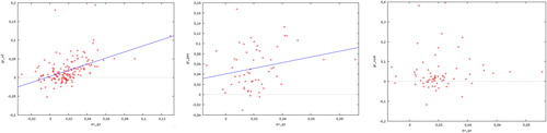
Figure 1 presents the scatter plot between average rate of economic growth and average rates of growth (respectively) of oil, natural gas and coal consumption.²³ A similar pattern can be seen in each case – with greater average rate of economic growth, greater rate of resource consumption is associated. Correlation coefficients are equal to (respectively) 0.49, 0.23 and 0.07.

Figure 1. Scatter plot between rate of economic growth and average rate of resource consumption – oil, natural gas and coal. Source: own calculations.

When the sample is limited to only O.E.C.D. countries the results are similar – correlation coefficients are equal to (respectively) 0.68, 0.24 and 0.005. Figure 2 shows these correlations. Figure 3 shows the correlation between given variables when a sample is restricted to non-O.E.C.D. members. Correlation coefficients are in that case (respectively) 0.5, 0.21 and 0.06. Figures 4–6 show a similar correlation for average growth rate of physical capital and respective rates of growth of natural resource use. Scatter plot Figures 7, 8 and 9 present correlations between average economic growth rate and rates of growth of DMC, respectively, for the whole sample, for O.E.C.D. countries only, and for non-O.E.C.D. countries. Table 2 contains correlation coefficients.

Figure 2. Scatter plot between the rate of economic growth and the average rate of resource consumption – oil, natural gas and coal, O.E.C.D. countries. Source: own calculations.

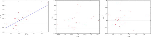
Figure 3. Scatter plot between the rate of economic growth and the average rate of resource consumption – oil, natural gas and coal, non-O.E.C.D. countries. Source: own calculations.

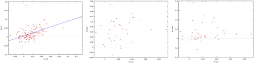
Figure 4. Scatter plot between the rate of growth of physical capital and the average rate of resource consumption – oil, natural gas and coal, all countries. Source: own calculations.

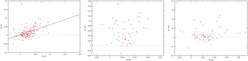
Figure 5. Scatter plot between the rate of growth of physical capital and the average rate of resource consumption – oil, natural gas and coal, O.E.C.D. countries. Source: own calculations.

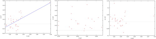
Figure 6. Scatter plot between the rate of growth of physical capital and the average rate of resource consumption – oil, natural gas and coal, non-O.E.C.D. countries. Source: own calculations.

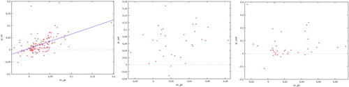
Figure 7. Scatter plot between the rate of economic growth (left) and the rate of growth of physical capital (right) and average rate of growth of DMC, all countries. Source: own calculations.

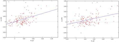
Figure 8. Scatter plot between the rate of economic growth (left) and the rate of growth of physical capital (right) and average rate of growth of DMC, O.E.C.D. countries. Source: own calculations.

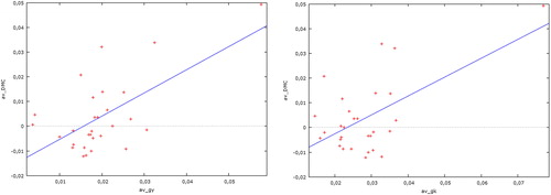
Figure 9. Scatter plot between the rate of economic growth (left) and the rate of growth of physical capital (right) and average rate of growth of DMC, non-O.E.C.D. countries. Source: own calculations.

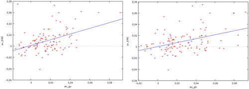
Table 2. The correlation between the average rate of economic growth or the average rate of growth of physical capital, and the average rate of growth of natural resources use.

Variable	Sample	groil	Noil	grgas	Ngas	grcoal	Ncoal	grDMC	NDMC
avgy	All	0.49	155	0.23	59	0.07	75	0.44	143
avgy	O.E.C.D.	0.68	30	0.24	23	0.005	30	0.62	29
avgy	Non-O.E.C.D.	0.5	125	0.21	36	0.06	45	0.44	114
avgk	All	0.5	155	0.15	59	–0.06	75	0.41	143
avgk	O.E.C.D.	0.66	30	–0.05	23	0.06	30	0.58	29
avgk	Non-O.E.C.D.	0.51	125	0.22	36	–0.04	45	0.40	114

Source: own calculations.

The results are as follows. First, the average rates of growth of natural resource consumption, which may be treated as natural resources used in production, are, on average, positive. Second, instead of a strictly negative correlation or correlation equal to 1, the data shows a positive correlation of moderate value, usually lower than 0.5 – with greater economic growth we observe, on average, greater natural resource extraction (except for coal, which seems not to be correlated with economic growth at all), but the relationships are far from strictly linear. This result does not depend on the subsample – similar results are found for all the countries, for O.E.C.D. countries and for non-O.E.C.D. countries, and do not depend on the kind of resource; it appears to be similar for coal, natural gas, oil and for materials in general.

5. Discussion and conclusions

The results obtained in the previous section stand in contradiction to the standard model, regardless of its version. The assumption of substitutability between physical capital and resources in the production process implies a negative correlation between natural resource use and economic growth. Despite this, data shows a positive correlation, so these two production factors are more likely to be complements or, at least, gross complements than substitutes. On the other hand, the level of complementarity is not strong, the expected linear relationship is out of range, and correlations are of a moderate size. Therefore both models and the implied predictions are incorrect and inconsistent with empirical evidence on a macro level in the long run.

We have used data of fossil fuels, which, in fact, are not standard natural resources. As an energy source²⁴ they are to some extent complements to physical capital. On the other hand, if strict complementarity is true, the correlation coefficient should be higher and closer to unity. Of course, oil and coal are also materials in the production process of some goods, so there might be some kind of substitutability. Data on domestic material consumption, on the other hand, shows similar correlations to that of fossil fuels, even though it contains a large share of minerals and metals. More detailed data is needed, for example for specific minerals and metals, such as copper and others, but this is also not available for a large cross-section of countries in a long enough period of time. Nevertheless, the use of this particular data set obviously affects the results, but there is no evidence or conjecture that this choice is not representative.

Complementarity is always presented in the same way, as in Equation (8)(8) $$Y^c=A\min {\{K,R\}}^{\gamma }{L}^{1-\gamma }$$(8) , but we assumed in Equation (7)(7) $$Y^s=A{K}^{\alpha }{R}^{\beta }{L}^{1-\alpha -\beta }$$(7) Cobb–Douglas substitutability between flow of non-renewable natural resources and other factors of production, particularly physical capital stock. This relation remains if we express the model in per capita terms – whenever an economy extracts and uses in production a small amount of natural resources it can still achieve a desirable level of production with, respectively, higher size of physical capital stock. So, an exponential decline in the extraction of natural resources can be compensated by an exponential increase in physical capital stock. There are other methods of including substitutability of factors of production in production function, such as, for example, the CES function.²⁵ Cobb–Douglas choice is dictated, again, by mathematical and presentational simplicity, and is widely used even in recently constructed models²⁶ – this kind of substitutability can be found, for example, in Stiglitz (1974), Acemoglu, Aghion, Bursztyn, and Hemous (2012), Golosov, Hassler, Krusell, and Tsyvinski (2014), Hassler, Krusell, and Olovsson (2012), Grimaud and Rougé (2014), and many others.

We use the correlation analysis instead of econometric estimation for two reasons: (1) in this situation the linear estimation should include only one explanatory variable, so the results of the estimations would give the same information as correlation coefficient analysis; and (2) there is no causality between these growth rates, at least this is not the obvious conclusion from the model, therefore econometric estimation seems not to be a proper tool. In addition, we notice that the entire group of countries may be considered as a population of all the countries that use a given resource. If so, it is not theoretically correct to provide a statistical significance of the correlation coefficient, therefore we did not perform this kind of test. The value of the correlation coefficient between the analysed variables is as it is and is sufficient to reach our goals.

In the majority of papers on economic growth and natural resource usage the assumption of substitutability between natural resource usage (as an energy source) and physical capital is made. Our research shows that this approach, even though it is quite standard, is not entirely correct. The models based on this approach are currently the basis for economic policy decisions, but results imply that a different approach is required, one that includes complementarity between the two factors. The implications of both approaches are different, but the data analysis leads us to the conclusion that complementarity seems to be closer to the real-world situation. Therefore, another step should be to propose a more complex mathematical model of economic growth and natural resource usage with complementarity between physical capital and flow of natural resource used in the production. In the future economic policy decision-making processes both models should be considered.

This research provides evidence in favour of complementarity between natural resources and physical capital, but the results are not conclusive. Strict complementarity is apparently not the case, but these production factors are more likely to be gross complements than substitutes. There exist, most probably, some forms of substitutability, but their existence is not in the scope of this paper.

Acknowledgements

The author would like to thank three anonymous referees for their valuable comments and participants of the mathematical economics conference in Poznań for many interesting suggestions. Special thanks to his dear wife for her endless support. The usual disclaimer applies. The publication of this paper was partially financed by the Dean of the Faculty of Economics and Sociology of the University of Lodz.

Disclosure statement

No potential conflict of interest was reported by the author.

Notes

Notes

1 See Malaczewski (2018) for a description of this issue.

2 Markandya and Pedroso-Galinato (2007), p. 299.

3 For θ = 1 utility function takes logarithmic form, $U(c)=\hspace{0.17em}\text{ln}\hspace{0.17em}(c)$.

4 We do not focus on the source of technical change – it might have been endogenous as well. There are plenty of approaches to modelling endogenous technological progress (Jones, 1995, Romer, 1990, and many others), but taking them into consideration will lead to similar conclusions. Exogeneity of g is assumed for mathematical simplicity.

5 We assume that the initial stock of available resources S(0) is known, which is obviously not the case in the real world. Nevertheless, even if it is not known, it is still finite and growth rates of basic macroeconomic variables do not depend on the level of S(0), so general conclusions are the same.

6 One can choose a different level of elasticity of substitution and, as a consequence, use the CES function instead of Cobb–Douglas, its special case. But when this elasticity is greater than 1, one of the production factors, physical capital or natural resource, becomes not essential in the production process, e.g., no natural resource (or physical capital) is needed for production, which obviously is not the case.

7 We assume for simplicity that one unit of physical capital requires exactly one unit of natural resource. Of course it is possible to consider a more general case when $Y^k=A\min {\{K,ϵ·R\}}^{\gamma }{L}^{1-\gamma }$ , where $ϵ$ is a parameter which expresses how many units of R are needed for one unit of K. Nevertheless, the conclusions are exactly the same in both cases (proof available on request), therefore we decide, again, for simplicity, to consider a less general case.

8 In the more complex analysis the variable elasticity of substitution (VES) production function (see Bairam, 1991) can be used. The VES function is considered to be more flexible but more mathematically complex. To keep the analysis simple, we decided to use Cobb–Douglas and Leontief production functions.

9 The discount rate is usually assumed to be close to $0.04-0.05$ (see, for example, Lucas, 1988) and the rate of population growth is considered to be close to $0.02-0.03$ , therefore $\rho -n$ is, in fact, positive. It is possible to consider the special case in which n = 0 (no population growth), which does not change any of the conclusions in our paper.

10 We shall skip the details of the calculations for simplicity, but they are available upon request from the author.

11 Transversality conditions (14) and (15) are fulfilled, which is straightforward to verify.

12 In this case transversality conditions are also fulfilled due to the fact that after $T^{*}$ there are no natural resources (so s = 0) and existing physical capital is gradually consumed.

13 A similar approach to empirical research based on long-run data is known in the literature on the subject. It can be observed, for example, in such fundamental papers as Barro (1991), Barro and Sala-i-Martin (1992), and many others.

14 Heston, Summers, and Aten (2012).

15 http://www.eia.gov.

16 S.E.R.I. – Sustainable Europe Research Institute, http://seri.at

17 Similar results were obtained for depreciation rate equal to 0.03, 0.04 and 0.06.

18 For most of the countries this is the year 1950, for some of them, 1970. This long period of time before the actual time span (1981–2010) ensures that the starting value of physical capital is irrelevant for most of the countries while calculating growth rates and average growth rate. Caselli (2005) proposes a balanced growth path assumption for K(0), which requires estimation of all macroeconomic parameters.

19 Even though we assume K = 0 at the starting period we receive a time series of rate of growth of physical capital per capita which we believe is quite close to the real one. Indeed, from Equation (22) it can be noticed that the starting level of physical capital is irrelevant due to the fact that ${(1-\delta )}^T$ is close enough to zero (δ is set at 0.05).

20 Similar results were obtained for compound growth rate. By taking average growth rates the situation when a country follows different paths of growth in the given period is not considered, which may be treated as a flaw of this study. Nevertheless, by using arithmetic mean, which is consistent with a standard approach in economic growth studies, we focus on the average growth paths and patterns. In this study each country is only a single observation in the group of almost all countries, which should not affect final results in a significant way.

21 Jones (1997) discovers an important difference between capital per worker and capital per capita time series in describing economic growth. We use capital per capita time series instead of capital/labour ratio due to availability of the data. We assume similarities between these time series, but probably this might be a reason for differences between g_k and g_y.

22 Lists of countries included in each subsample are available on request.

23 On every figure on the horizontal axis there is average rate of economic growth and on the vertical axis average rate of growth of a particular resource. Each dot represents one economy. In some cases, where the correlation coefficient is of a higher value and the relation is more apparent, the regression line is added.

24 Csereklyei, Rubio-Varas, and Stern (2016) analyse panel data to provide some stylised facts connected with energy and economic growth. Their results, however, are not strictly related to natural resources use.

25 For example, Grimaud and Rougé (2008), Growiec and Schumacher (2008), and others.

26 Of course there are also other interesting, from a neoclassical perspective, properties of the Cobb–Douglas function, for example fulfilling Inada conditions. Baumgärtner (2004) proves that in the case of natural resource choice of this particular production function may not be suitable.

References

- Acemoglu, D. (2009). Introduction to modern economic growth. Princeton: MIT press.
- Acemoglu, D., Aghion, P., Bursztyn, L., & Hemous, D. (2012). The environment and directed technical change. The American Economic Review, 102(1), 131–166. doi: 10.1257/aer.102.1.131
- Apostolakis, B. E. (1990). Energy-capital substitutability/complementarity: The dichotomy. Energy Economics, 12(1), 48–58. doi: 10.1016/0140-9883(90)90007-3
- Arnberg, S., & Bjorner, T. B. (2007). Substitution between energy, capital and labour within industrial companies: A micro panel data analysis. Resource and Energy Economics, 29(2), 122–136. doi: 10.1016/j.reseneeco.2006.01.001
- Bairam, E. (1991). Functional form and new production functions: Some comments and a new VES function. Applied Economics, 23(7), 1247–1250. doi: 10.1080/00036849100000164
- Barro, R. J. (1991). Economic growth in a cross section of countries. The Quarterly Journal of Economics, 106(2), 407–443. doi: 10.2307/2937943
- Barro, R. J., & Sala-I-Martin, X. (1992). Convergence. Journal of Political Economy, 100(2), 223–251. doi: 10.1086/261816
- Barro, R. J., & Sala-I-Martin, X. (2003). Economic growth (2nd ed.). Cambridge: MIT press.
- Baumgärtner, S. (2004). The Inada conditions for material resource inputs reconsidered. Environmental and Resource Economics, 29, 307–322.
- Caselli, F. (2005). Accounting for cross-country income differences. Handbook of Economic Growth, 1, 679–741.
- Cohen, F., Hepburn, C., & Teytelboym, A. (2017). Can we stop depleting natural capital? A literature review on substituting it with other forms of capital. INET Oxford Working Paper No. 2017-13.
- Costantini, V., & Paglialunga, E. (2014). Elasticity of substitution in capital-energy relationships: How central is a sector-based panel estimation approach? (No. 1314). Sustainability Environmental Economics and Dynamics Studies.
- Costanza, R., & Daly, H. E. (1992). Natural capital and sustainable development. Conservation Biology, 6(1), 37–46. doi: 10.1046/j.1523-1739.1992.610037.x
- Csereklyei, Z., Rubio-Varas, M., & Stern, D. I. (2016). Energy and Economic Growth: The Stylized Facts. The Energy Journal, 37(2), 223–255.
- Daly, H. E. (1997). Georgescu-Roegen versus Solow/Stiglitz. Ecological Economics, 22(3), 261–266. doi: 10.1016/S0921-8009(97)00080-3
- Daly, H. E. (1999). How long can neoclassical economists ignore the contributions of Georgescu-Roegen? In Bioeconomics and Sustainability: Essays in Honour of Nicholas Georgescu-Roegen (pp. 13–24). Cheltenham, UK: Edward Elgar Publishing.
- Georgescu-Roegen, N. (1979). Energy analysis and economic valuation. Southern Economic Journal, 45(4), 1023–1058. doi: 10.2307/1056953
- Golosov, M., Hassler, J., Krusell, P., & Tsyvinski, A. (2014). Optimal taxes on fossil fuel in general equilibrium. Econometrica, 82(1), 41–88.
- Grimaud, A., & Rougé, L. (2008). Environment, directed technical change and economic policy. Environmental and Resource Economics, 41(4), 439–463.
- Grimaud, A., & Rougé, L. (2014). Carbon sequestration, economic policies and growth. Resource and Energy Economics, 36(2), 307–331. doi: 10.1016/j.reseneeco.2013.12.004
- Growiec, J., & Schumacher, I. (2008). On technical change in the elasticities of resource inputs. Resources Policy, 33(4), 210–221. doi: 10.1016/j.resourpol.2008.08.006
- Hassler, J., Krusell, P., & Olovsson, C. (2012). Energy-saving technical change (No. w18456), National Bureau of Economic Research.
- Heston, A., Summers, R., & Aten, B. (2012). Penn World Table Version 7.1, Center for International Comparisons of Production, Income and Prices at the University of Pennsylvania, Nov.
- Jones, C. I. (1995). R & D-based models of economic growth. Journal of Political Economy, 103(4), 759–784. doi: 10.1086/262002
- Jones, C. I. (1997). On the evolution of the world income distribution. The Journal of Economic Perspectives, 11(3), 19–36. doi: 10.1257/jep.11.3.19
- Koetse, M. J., De Groot, H. L., & Florax, R. J. (2008). Capital-energy substitution and shifts in factor demand: A meta-analysis. Energy Economics, 30(5), 2236–2251. doi: 10.1016/j.eneco.2007.06.006
- Lucas, R. E. (1987). On the mechanics of economic development. Journal of Monetary Economics, 22, 3–42. doi: 10.1016/0304-3932(88)90168-7
- Malaczewski, M. (2018). Natural resources as an energy source in a simple economic growth model. Bulletin of Economic Research, 70(4), 362–380. doi: 10.1111/boer.12153
- Markandya, A., & Pedroso-Galinato, S. (2007). How substitutable is natural capital?. Environmental and Resource Economics, 37(1), 297–312. doi: 10.1007/s10640-007-9117-4
- Mehra, R., & Prescott, E. C. (1985). The equity premium: A puzzle. Journal of Monetary Economics, 15(2), 145–161. doi: 10.1016/0304-3932(85)90061-3
- Romer, P. M. (1990). Endogenous technological change. Journal of Political Economy, 98(5, Part 2), S71–S102. doi: 10.1086/261725
- Solow, J. L. (1987). The capital-energy complementarity debate revisited. The American Economic Review, 77(4), 605–614.
- Solow, R. M. (1997). Georgescu-Roegen versus Solow-Stiglitz. Ecological Economics, 22(3), 267–268. doi: 10.1016/S0921-8009(97)00081-5
- Stiglitz, J. (1974). Growth with exhaustible resources: Efficient and optimal growth paths. Review of Economic Studies, (symposium volume), 123–137. doi: 10.2307/2296377
- Stiglitz, J. (1997). Georgescu-Roegen versus Solow-Stiglitz. Ecological Economics, 22(3), 269–270. doi: 10.1016/S0921-8009(97)00092-X
- Szpiro, G. G. (1986). Measuring risk aversion: An alternative approach. The Review of Economics and Statistics, 68(1), 156–159. doi: 10.2307/1924939