Determinants of price fluctuations in the electricity market: a study with PCA and NARDL models

Abstract

In the modern electricity markets, negative prices and spike prices coexist as a pair of opposite economic phenomena. This study investigates how these extreme prices play as the determinants to drive price fluctuations in the electricity market. We construct a two-stage analysis including a principal component analysis (PCA) and a nonlinear autoregressive distributed lags model (NARDL). We apply this analytical method to the wholesale Pennsylvania, New Jersey and Maryland (PJM) electricity market. We find that according to PCA, in the individual transmission lines, spike prices are determinants with largest explanatory power to the variation of prices, while according to NARDL, from the standpoint of the overall market, negative prices have a larger potential effect on both the real-time market and the forward market. These results are valuable and contributive to managers and operators in the electricity markets for policy decision making.

Keywords:

• Price fluctuation
• principal component analysis
• NARDL
• electricity market
• spike price
• negative price

JEL CLASSIFICATION:

• C12
• C22
• G19
• Q49

1. Introduction

The trend of modern electricity system reform in all major countries of the world is market-oriented. The modern electricity system is no longer an electric transmission grid only. It has been a wholesale energy market style with new multiple functions. Besides energy production and transmission, the electricity market is also responsible to secure reliable electricity supply, manage the energy prices and consequently improve market efficiency.

The marketisation of the electricity system brings more market phenomena. The original transmission organisation has become a wholesale market where the wholesale price of electricity is matched between generators and demanders. Like the financial markets, the electricity market takes the electricity prices to reflect the energy demand and supply. Along with the development of the wholesale electricity market restructuring and the adoption of auction mechanisms, like the financial markets, large fluctuations of electricity price have been observed frequently. The growth of price fluctuations in the electricity markets gains attention from academia, and these ‘extreme price swings’ have been viewed as a symbolic feature of electricity markets (Engle & Patton, 2001; Hadsell, Marathe, & Shawky, 2004; Knittel & Roberts, 2005; Xiao, Colwell, & Bhar, 2015; Zareipour, Bhattacharya, & Cañizares, 2007).

Previous studies regarding the price swings generally focus on the prevalence of spike prices, that is, the extremely high prices (Carlton, 1977; Crew & Kleindorfer, 1976; Hadsell & Shawky, 2006; Joskow & Wolfram, 2012; Nguyen, 1976; Spees & Lave, 2008; Wenders, 1976). Spike prices generate high marginal costs for the excess demand and thus enlarge the price uncertainty in the peak load scenarios. Therefore, spike prices are usually considered as the cause of price fluctuations.

But recently, an increasing number of negative prices appear in the electricity market as another type of extreme prices, which quickly becomes a distinctive feature of the electricity market. The occurrence of negative pricing arises because certain types of generators (e.g., nuclear, hydroelectric, and wind energy) pay demanders to take power instead of lowering their output due to technical and economic factors, even when demand is insufficient to absorb their output ( U.S. Energy Information Administration, 2012a, 2012b ). As the opposite situation of spike prices, negative prices represent the extreme over-supply of electric power, which is not a good signal for market equilibrium (Baradar & Hesamzadeh, 2014; Barbour, 2014; Genoese, Genoese, & Wietschel, 2010; Sioshansi, Denholm, Jenkin, & Weiss, 2009; Zhou et al. 2016).

Although many previous studies suggest the price swings in the electricity market as a critical research target, however, most studies focus on one type of extreme prices only. According to economics, the negative price and the spike price are a pair of opposite phenomena. The negative price implies the over-supply while the spike price implies the over-demand. Both types of extreme prices are constituent of price swings. Therefore, it is necessary to understand how the large price swing is formed, which price behaviour is the primary factor of the extreme price swing, and how the price swing impacts the electricity market.

This study observes both spike and negative prices in the wholesale electricity market, and explores how they contribute to the price fluctuations of the market. The purpose of this study is important, because assessing the two opposite prices and the economic phenomena behind them can help the managers and operators of the electricity markets better know about the market status and thus let them make the correct and reasonable decision for market stability.

This study explores the price fluctuation in a multi-area and multiple transmission line environment. Existing studies regarding price fluctuation usually focus on a single area with one single series of data (Hadsell et al., 2004; Hadsell & Shawky, 2006; Holland & Mansur, 2006). However, since electricity markets were restructured in the last decade, the modern electricity market usually include a large number of transmission lines across diverse geographic areas. Following the market reform, we choose the wholesale Pennsylvania, New Jersey and Maryland (PJM) electricity market as our research target. The PJM market is the oldest electricity transition system and the second largest wholesale electricity market in the world. It coordinates the movement of power in 13 states and the District of Columbia, including over 240,000 square miles of territory, 84,000 miles of transmission lines and 65 millions of people. It includes over 11,000 transmission lines with hourly updated electricity prices. Findings from the PJM market can provide valuable lessons and experiences for other electricity markets.

Inspired by a series of recent literature, this study designs a two-step research procedures. First, following (Baek, Cursio, & Cha, 2015; Chakrabarty & Tyurin, 2011; Li, Cursio, & Sun, 2018) we construct a Principal Component Analysis (PCA) model to explore the negative and spike prices in each individual transmission line from PJM market, and see how the two types of prices affect the price fluctuation from the dimension of individual transmission lines. This micro-level analyses can bring latent insights to the managers and operators of the electricity markets. Second, we construct the nonlinear autoregressive distributed lags model (NARDL), and use it to assess the determinant of price fluctuation from the angle of the overall electricity market. Results from the NARDL model can shed light on market supervision and help market operators make decisions on the policy making and regulation adjustments.

Through the results of PCA we select six components and interpret their implication related to the covariates. We find that components with the largest explanatory power to the variation of prices are highly related to spike LMPs and the position and the extent of concentration of the overall LMPs. Therefore, in the dimension of the individual transmission lines, there exists over-demand with a high frequency. Different from PCA, results of the NARDL model suggest that the negative prices have a larger potential effect on both the real-time market and the forward market. As an implication, this finding confirms the contribution of the renewable energy incentive mechanisms, and believes that the renewable energy will fulfil the energy demand and help balance the energy equilibrium in the future.

The remainder of this paper is organised as follows. Section 2 introduces previous literature and research methodology. Section 3 describes the PJM market, data and covariates. Section 4 presents results of the PCA and NARDL models and implications. Section 5 concludes.

2. Literature review and methods

2.1. Literature review

As a special type of energy, electricity cannot be stored in large quantities. Therefore, the electricity market is widely viewed as the most difficult market to balance between supply and demand. For example, He and Victor (2017) study the electricity system in China after Chinese government provided access to electricity to its entire population in 2015. They summarise lessons and experiences about electricity supply in this large emerging countries and figure out that the power equilibrium is too hard to achieve. Yang (2017) also takes Chinese electricity system as the target and points out that the power equilibrium and efficiency are not achieved yet even after installing advanced metering infrastructure. Li, Cursio, Jiang, and Liang (2019) study the U.S. smart grid electricity system and find that the abnormal price movement in the electricity market, which is viewed as a signal of the inequilibrium between supply and demand, is relevant to calendar issues with significance.

Thus, previous studies have widely acknowledged that it is extremely challenging for electricity generators (especially those with unstable output) to fulfil the demand with a fixed amount of supply. As stated by existing studies (Bilitewski, 2012; Frömmel, Han, & Kratochvil, 2014; Yuan, Bi, & Moriguichi, 2006) , a stable price level is a signal of inequilibrium between power supply and demand. Reduction in price swings is an achievement of both market efficiency and resource efficiency. Therefore, many studies pay attention to price swings, and contribute to its reduction from aspects of methodologies and phenomena.

Many studies focus on the extreme price values in the electricity market, and try to explore their trend and patterns. These studies can be sorted in two groups. One group of studies focus on the extremely high price records, which are usually called spike prices. They attribute the price swings to the prevalence of spike price. For example, Hadsell and Shawky (2006) focus on the high prices during peak hours, and examine the volatility characteristics of the New York Independent System Operator (NYISO) electricity markets. They find evidence that links the occurrence of spike prices and market price volatility. Joskow and Wolfram (2012), Dutta and Mitra (2017) introduce the progress of spike pricing in the electricity market, and discuss candidate technologies which could reduce spike pricing and thus control the proliferation of time-varying electricity pricing.

Another group of studies focus on negative pricing, which is the distinctive phenomenon in the electricity market other than the other financial markets. The occurrence of negative pricing arises because certain types of generators (e.g., nuclear, hydroelectric, and wind energy) pay demanders to take power instead of lowering their output due to technical and economic factors, even when demand is insufficient to absorb their output ( U.S. Energy Information Administration, 2012a, 2012b). Genoese et al. (2010) find that negative pricing has an increasing trend and unbalanced distribution in German markets, and it enlarges the price volatility. Barbour, (2014) state that negative pricing is the key factor to the energy efficiency and directly affects the development of relevant technologies, such as energy storage. Therefore, like spike prices, negative prices are also critical factors to the price swings in the electricity market.

Some existing studies suggest that the electricity market is driven by specific factors with dominant power. For example, Simanaviciene, Virgilijus, and Simanavicius (2017) investigate the psychological factors and their influences on energy efficiency in households, in order to identify and track individual’s energy consumption behaviour. Therefore, we consider exploring the factors with dominant effects on electricity market price swings by using factor-related methods. One candidate method is NARDL, in which nonlinearities are introduced via positive and negative partial sum decompositions of the explanatory variables (Shin, Yu, & Greenwood-Nimmo, 2013). A number of studies show that NARDL is an ideal tool to examine prices relations (Ibrahim, 2015; Jammazi, Lahiani, & Nguyen, 2015; Nusair, 2017; Shin et al., 2013). For example, Ibrahim (2015) examines the relations between food and oil prices for Malaysia using a nonlinear ARDL model. Jammazi et al. (2015) use a wavelet-based NARDL to investigate the fluctuations in the exchange rates and its impact on crude oil prices.

Another method is PCA, which is considered as one of the most widely used techniques in multivariate statistical inference. Recent studies summarise the advantages of PCA into three aspects: (1) PCA reduces the dimensionality of the multivariate statistical problems, replacing a number of variables a smaller number of PCs which effectively summarise a previously large part of the variation of the data (Baek et al., 2015; Bai, 2003; Bai & Ng, 2002; Stock & Watson, 1998, 2002); (2) PCA is a preferable approach for studies with large data sizes (Aït-Sahalia & Xiu, 2019; Cao & Huang, 2007; Skiadopoulos, Hodges, & Clewlow, 2000); (3) PCA constructs latent common structure of factors and discovers the structural meaning (Chakrabarty & Tyurin, 2011; Forni, Hallin, Lippi, & Reichlin, 2000, 2004; Forni & Lippi, 2001). In this study, we follow the structure of method in Li, Cursio, and Sun (2018) and build our PCA model.

Following the existing studies, in this paper we plan to explore both spike and negative prices. It is new by comparison with the previous studies which focus on one type of extreme prices only. From the perspective of economics, spike prices reflect the over demand while negative prices reflect over supply. The managers and operators of the electricity markets need to know about the patterns and trends of the market prices movement, and consequently have appropriate preparations for different types of extreme cases. Moreover, the existing studies suggest that the factor-related analytical methods are powerful tools for studies with big data. Therefore, as another research target, in this paper we use the NARDL and PCA methods as the effective tools to explore the price fluctuations in the electricity market. This paper is an extension of the previoius study (Li, Cursio, & Sun, 2018).

2.2. NARDL framework

In this study we use the NARDL approach proposed by Shin et al. (2013). The basic model is described as follow: (1) $$y_t=\sum _{j=1}^p{\mathrm{\varnothing }}_j{y}_{t-j}+\sum _{j=0}^q{\theta }_j^{+\prime }{x}_{t-j}^{+}+\sum _{j=0}^q{\theta }_j^{-\prime }{x}_{t-j}^{-}+{\epsilon }_t$$(1)

Where the dependent variable $y_t$ and its lag length $y_{t-1}$ are scalar variable, $x_{t-j}^{+}$ and $x_{t-j}^{-}$ are decomposed independent variables.

The NARDL model has advantages for large data since it yields valid results regardless of whether the underlying variables are integrated of order one, zero, or a combination of both (Pesaran, Shin, & Smith 2001). According to Shin et al. (2013), Jammazi et al. (2015) and Nusair (2017), in the NARDL model the existence of a long-run relationship among a set of variables can be tested without any prior knowledge about the order of integration of the individual variables, which avoids problems associated with unit roots pre-testing. Moreover, both the dependent variable and independent variables can be introduced in the model with lags, which makes the test procedure more flexible than the other methods.

2.3. PCA framework

In this section we briefly review the mathematical mechanism of PCA. Principal Component Analysis is one of the most widely used techniques in multivariate statistical inference. From the perspective of mathematics, if there are a series of variables that are related, PCA can transform them into the same number of uncorrelated new variables. Suppose we have a column vector of n random variables $\mathit{x}={\left[x_1,x_2,\dots ,\mathrm{ }{x}_n\right]}^T$ and its mean vector is a zero vector (E[x] = 0). Since these n random variables $\mathit{x}={\left[x_1,x_2,\dots ,\mathrm{ }{x}_n\right]}^T$ are suspiciously related, we need to transform them into normalized linear combinations and find which combination explains most of the total variability. In mathematics, we look for a non-zero column vector $\mathit{B}\mathrm{ }={\left[{\mathrm{b}}_1,{\mathrm{b}}_2\dots b_n\right]}^T$ which satisfies ${\mathit{B}}^{\mathrm{\text{'}}}\mathit{B}=1$, in order to maximize the variance of the linear combination, B’x. The variance of B’x can be written as (2) $$\mathit{Var}\left[\mathit{B}\mathrm{’}\mathit{x}\right]=E{\left[{\mathit{B}}^{\mathrm{\text{'}}}\mathit{x}\right]}^2=E\left[{\left(b_1{x}_1+b_2{x}_2+\dots +b_n{x}_n\right)}^2\right]$$(2)

Since the covariance matrix of x is C, the variance of B’x can be written as (3) $$\mathit{Var}\left[\mathit{B}\mathrm{’}\mathit{x}\right]={\mathit{B}}^{\mathrm{\text{'}}}\mathit{C}\mathrm{ }\mathit{B}$$(3)

To find B, we solve the following Lagrange function (4) $$L={\mathit{B}}^{\mathrm{\text{'}}}\mathit{C}\mathrm{ }\mathit{B}-\lambda ({\mathit{B}}^{\mathrm{\text{'}}}\mathit{B}-1)$$(4) where λ is a Lagrange multiplier. As the first order condition (FOC), the vector of partial derivative is (5) $$\frac{\partial L}{\partial \mathit{B}}=2\mathrm{ }\mathit{C}\mathrm{ }\mathit{B}-2\mathrm{ }\lambda \mathrm{ }\mathit{B}=2\left(\mathit{C}-\lambda \mathrm{ }\mathit{I}\right)\mathit{B}=0$$(5)

We can simplify the FOC into the equation $\mathit{C}\mathrm{ }\mathit{B}=\mathrm{ }\lambda \mathrm{ }\mathit{B}$, which conforms to the expression of the eigenvalue. Therefore, λ is the eigenvalue to the covariance matrix C, and B is the corresponding eigenvector. To each ${\lambda }_i$ ($i=1,2,\dots n$), the corresponding eigenvector ${\mathit{B}}_{\mathit{i}}$ has the explanatory power of the total variability. ${\mathit{B}}_{\mathit{i}}^{\mathrm{\text{'}}}\mathit{x}$, the linear combination, is the principal component (PC) of x with variance equal to ${\lambda }_i$.

Finally, we have a total of n PCs, which are independent to each other, as the substitution of x to explain the variability. (6) $$\begin{array}{c}P{C}_1={\mathit{B}}_1^{\mathrm{\text{'}}}\mathit{x}=b_{11}{x}_1+b_{12}{x}_2+\dots +b_{1n}{x}_n\\ P{C}_2={\mathit{B}}_2^{\mathrm{\text{'}}}\mathit{x}=b_{21}{x}_1+b_{22}{x}_2+\dots +b_{2n}{x}_n\\ \dots \dots \\ P{C}_n={\mathit{B}}_{\mathit{n}}^{\mathrm{\text{'}}}\mathit{x}=b_{n1}{x}_1+b_{n2}{x}_2+\dots +b_{\mathit{nn}}{x}_n\end{array}$$(6)

The PCs keep most of the important information contained in the original variables x. PCA enables us to identify the PCs as a new set of orthogonal factors.

3. PJM, data and covariates

3.1. PJM market

In this section we introduce the PJM electircity market. PJM was established in 1927 and is currently the leading electricity transition system in the world. Early in 1962, PJM installed its first online computer to control generation and then established the first energy management system (EMS). In 1997, PJM opened its first bid-based energy market and evolved into the largest deregulated wholesale electricity market in the world. In 2013, PJM launched a new stage smart-grid development and implemented the Advanced Control Center in order to ensure uninterrupted operation of the electric system and maintain the steadiness of the electric market.

More importantly, PJM serves as a clearing house of electricity power. Market participants, including the power generators and consumers, offer and bid for electricity on a real-time basis. PJM matches bids and offers and gives the market-clearing price within minutes of the spot trade. Then electricity will be generated and transmitted to each service area. PJM is not only an electric system, it conveys more functions like the financial markets, as discussed by Bessembinder and Lemmon (2002), Geman and Roncoroni (2006), Longstaff and Wang (2004), and Seifert and Uhrig-Homburg (2007).

Today, PJM is the biggest regional transmission organisation (RTO) of power in the United States, and coordinates the movement of power in 13 states and the District of Columbia. Areas served by PJM are divided by the transmission lines which are referred to as the pricing nodes (Pnode). The market-clearing price is referred to as the locational marginal price (LMP) and updated hourly. LMP is the sum of the cost of energy, the marginal cost of transmission loss, and the marginal cost of congestion, which are the leading contributors to volatility in electricity prices. It represents the incremental value of an additional MW of power transported to a particular Pnode.

Thus, in this study we take PJM as the research target and treat it as a market from the perspective of finance and economics. Findings from PJM will shed light on the efficient management on electricity markets.

3.2. Data and covariates

We use the hourly LMP data during 2013–2016 including distinct 11,574 Pnodes. Table 1 presents the descriptive statistics of LMPs. There are about 392 million LMP records on these Pnodes. We identify all the non-positive LMP records as the negative pricing. There are over two million negative LMPs, which count for about the bottom 1% of the total LMPs. Likewise, we distinguish the spike LMPs as the top 1% LMPs for each Pnode as a consistency of previous studies (Walawalkar, Blumsack, Apt, & Fernands, 2008). The mean of negative LMPs is −$26.22 and the mean of the spike LMPs is $326.21. The standard deviation of negative LMPs is 47.37 while the standard deviation of spike LMPs is 240.14. The overall ranges of both groups are wide: negative LMPs spread between −$2240.3 and 0 whereas the spike LMPs spread between $175.96 and $4643.74. The distribution of negative and spike LMPs are depicted in Figure 1.

Figure 1. Histogram for the occurrence of negative and spike LMPs.

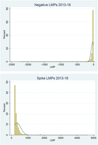
Table 1. Descriptive statistics of LMPs.

Variable	Negative LMP	Spike LMP	Overall
Number of Occurrence	2,067,194	3,943,996	392,216,015
mean	−26.22	326.21	35.62
Std. Dev.	47.37	240.14	42.61
skewness	−7.06	4.05	17.15
kurtosis	135.88	22.99	545.14
min	−2240.30	175.96	−2240.30
p5	−107.05	179.70	14.88
p25	−30.48	202.72	23.43
p50	−9.54	250.75	28.46
p75	−2.7	351.66	36.45
p95	0	689.57	72.68
max	0	4643.74	4643.74

We sort the three categories of LMPs, overall, negative and spike, by their Pnode IDs. For the overall LMPs of each Pnode, we calculate the mean, skewness and kurtosis. For the other categories in each Pnode, we calculate the descriptive statistics, including mean, standard deviation, skewness, kurtosis, minimum, and maximum. We also calculate the percentage of occurrence for each group across Pnodes. For Pnode i, the percentage of negative LMPs is defined as

(7) $$\mathit{Neg}\_\mathit{Pe}{r}_i=\frac{\mathit{Number}\mathrm{ }\mathit{of}\mathrm{ }\mathit{Occurrence}\mathrm{ }\mathit{of}\mathrm{ }\mathit{negative}\mathrm{ }\mathit{LMPs}}{\mathit{Total}\mathrm{ }\mathit{Number}\mathrm{ }\mathit{of}\mathrm{ }\mathit{LMPs}\mathrm{ }\mathit{for}\mathrm{ }i}$$(7)

And the percentage of spike LMPs is defined as

(8) $$\mathit{Peak}\_\mathit{Pe}{r}_i=\frac{\mathit{Number}\mathrm{ }\mathit{of}\mathrm{ }\mathit{Occurrence}\mathrm{ }\mathit{of}\mathrm{ }\mathit{Peak}\mathrm{ }\mathit{Load}\mathrm{ }\mathit{Spike}\mathrm{ }\mathit{LMPs}}{\mathit{Total}\mathrm{ }\mathit{Number}\mathrm{ }\mathit{of}\mathrm{ }\mathit{LMPs}\mathrm{ }\mathit{for}\mathrm{ }i}$$(8)

For further analyses we use the 16 covariates listed in Table 2. These covariates are categorised into three categories of LMPs. We exclude the maximum of negative LMPs because it is zero in all Pnodes.

Table 2. Covariates of PCA.

variable	Negative LMPs	Spike LMPs	Overall
Percentage of Occurrence	Neg_Per	Peak_Per
mean	Neg_Mean	Peak_Mean	Mean
Std. Dev.	Neg_Std	Peak_Std
skewness	Neg_Sku	Peak_Sku	Skewness
kurtosis	Neg_Kur	Peak_Kur	Kurtosis
min	Neg_Min	Peak_Min
max		Peak_Max

4. Results and implication

In this section, we give our analyses and results in two steps. First, following Li et al. (2018), we use PCA model to explore the determinants of electricity prices across Pnodes. The results are from the standpoint of individual transmission lines (Pnodes) to observe the price swings. Second, we use NARDL model to see how these extreme prices and the energy inequilibrium behind them affect the stability of the whole market. The results are from the standpoint of the overall electricity market, which can bring more insights for market managers and operators.

4.1. PCA results

Table 3 presents the variation explained by the eigenvalues of PCA. PC1, the component that has the largest eigenvalue 5.67, contributes 35% explanatory power to the variation of data. PC2 has the second largest eigenvalue (3.36) and explains 21% of the variation. The cumulative explanatory contribution by PC1 and PC2 has reached 56% as shown in the cumulative column. Including the first six components, the cumulative explanatory contribution by PC1 – PC6 already reaches up to 98%. Therefore, PCA helps reduce the dimensionality.

Table 3. Variations explained by the eigenvalues of PCA.

Component	Eigenvalue	Difference	Proportion	Cumulative
PC1	5.67	2.31	0.35	35%
PC2	3.36	0.28	0.21	56%
PC3	3.08	1.11	0.19	76%
PC4	1.98	1.10	0.12	88%
PC5	0.88	0.22	0.06	94%
PC6	0.67	0.55	0.04	98%
PC7	0.12	0.03	0.01	99%
PC8	0.09	0.04	0.01	99%
PC9	0.05	0.01	0.00	99%
PC10	0.04	0.02	0.00	100%
PC11	0.02	0.01	0.00	100%
PC12	0.01	0.00	0.00	100%
PC13	0.01	0.00	0.00	100%
PC14	0.01	0.00	0.00	100%
PC15	0.00	0.00	0.00	100%
PC16	0.00	.	0	100%

We extract the first six components. They are constructed as linear combinations of covariates so that they have orthonormal loading coefficients. Table 4 presents how these PCs relate to our covariates and lists the coefficients of covariates for each PC in the columns. For example, PC1 is expressed as the linear combination of our original covariates by the following equation: (9) $$\mathit{PC}1\mathrm{ }=\mathrm{ }0.3697M\mathit{ean}\mathrm{ }-\mathrm{ }0.3410S\mathit{kewness}\mathrm{ }-\mathrm{ }0.37K\mathit{urtosis}\mathrm{ }-\mathrm{ }0.0947N\mathit{eg}\_\mathit{Per}\mathrm{ }-\mathrm{ }0.0347N\mathit{eg}\_\mathit{Min}\mathrm{ }-\mathrm{ }0.0925N\mathit{eg}\_\mathit{Mean}\mathrm{ }+\mathrm{ }0.0926\mathrm{ }\mathit{Neg}\_\mathit{Std}\mathrm{ }+\mathrm{ }0.0639N\mathit{eg}\_\mathit{Sku}\mathrm{ }-\mathrm{ }0.0810N\mathit{eg}\_\mathit{Kur}\mathrm{ }+0.3177P\mathit{eak}\_\mathit{Per}\mathrm{ }+\mathrm{ }0.3704P\mathit{eak}\_\mathit{Min}\mathrm{ }+\mathrm{ }0.3742P\mathit{eak}\_\mathit{Mean}\mathrm{ }+\mathrm{ }0.1286P\mathit{eak}\_\mathit{Std}\mathrm{ }-\mathrm{ }0.3020P\mathit{eak}\_\mathit{Sku}\mathrm{ }-\mathrm{ }0.2868P\mathit{eak}\_\mathit{Kur}\mathrm{ }+\mathrm{ }0.0641P\mathit{eak}\_\mathit{Max}$$(9)

Table 4. Covariate coefficients of six PCs.

Covariate	PC1	PC2	PC3	PC4	PC5	PC6
Mean	0.3697	0.1928	0.0934	0.0365	0.2326	−0.0640
Skewness	−0.3410	0.2816	0.1046	0.0804	−0.0714	−0.0012
Kurtosis	−0.3700	0.1999	0.1216	0.0742	−0.0197	−0.0134
Neg_Per	−0.0947	−0.3074	0.1834	−0.0022	0.1819	0.8583
Neg_Min	−0.0347	0.2896	−0.4527	0.1104	0.0767	0.0454
Neg_Mean	−0.0925	0.2929	−0.3811	−0.2543	0.2246	0.1397
Neg_Std	0.0926	−0.2810	0.4240	0.1003	−0.2452	−0.2561
Neg_Sku	0.0639	−0.0759	−0.1459	0.6509	−0.0667	0.1845
Neg_Kur	−0.0810	−0.0217	0.2285	−0.6219	0.1353	0.0175
Peak_Per	0.3177	0.0361	0.1899	0.1168	0.5363	0.0058
Peak_Min	0.3704	0.1905	0.0920	0.0368	0.2328	−0.0624
Peak_Mean	0.3742	0.2081	0.0676	−0.0577	−0.1353	0.1449
Peak_Std	0.1286	0.4198	0.1842	−0.0573	−0.4019	0.2727
Peak_Sku	−0.3020	0.2032	0.2681	0.1658	0.2431	−0.0696
Peak_Kur	−0.2868	0.1511	0.2822	0.1924	0.3669	−0.0996
Peak_Max	0.0641	0.4160	0.3064	0.0565	−0.2298	0.1533

In Equation (9)(7) $$\mathit{Neg}\_\mathit{Pe}{r}_i=\frac{\mathit{Number}\mathrm{ }\mathit{of}\mathrm{ }\mathit{Occurrence}\mathrm{ }\mathit{of}\mathrm{ }\mathit{negative}\mathrm{ }\mathit{LMPs}}{\mathit{Total}\mathrm{ }\mathit{Number}\mathrm{ }\mathit{of}\mathrm{ }\mathit{LMPs}\mathrm{ }\mathit{for}\mathrm{ }i}$$(7) , among the covariates, four of them have significantly larger coefficients: Peak_Mean (0.3742), Peak_Min (0.3704), Kurtosis (-0.37) and Mean (0.3697). These covariates are the dominant power to constitute PC1. They represent the position of spike LMPs (Peak_Mean and Peak_Min), and the position and the extent of concentration of the overall LMPs (Kurtosis and Mean).

Similarly, in PC2, we find that two covariates have significantly larger absolute values of coefficients: Peak_Std (0.4198) and Peak_Max (0.4160). Both covariates are different from the dominant covariates for PC1, and are from the spike LMP group. Similar to PC1, PC2 can be interpreted as the distribution and dispersion of spike LMPs.

For PC3, three covariates are dominant as observed in Table 4: Neg_Min (−0.4527), Neg_Std (0.4240) and Neg_Mean (−0.3811). PC3 can be interpreted as the position and distribution of negative spike LMPs. Similarly, PC4’s dominant covariates are also the skewness and kurtosis of negative LMPs (Neg_Sku and Neg_Kur). So PC4 is also a representative of negative LMP group. But compared with PC2, both PC3 and PC4 have less explanatory power.

There is only one covariate that dominates in PC5 and PC6 respectively. In PC5, the only covariate is Peak_Std (−0.4019), and in PC6 it is Neg_Per (0.8583). As shown in Table 3, PC5 and PC6 have less explanatory power. They are supplementary variation.

In summary, through the result of PCA we select six components and interpret their implication related to the covariates. We find that components with the largest explanatory power to the variation of prices are highly related to spike LMPs and the position and the extent of concentration of the overall LMPs. Therefore, in the next part, we further examine the determinants from the perspective of the overall electricity market.

4.2. NARDL results

Results from PCA suggest that features from the overall market are critical to interpret the variation of electricity market prices. In this part, we further examine how these extreme prices and the energy inequilibrium behind them affect the stability of the whole market. Different from the PCA results which focus on the variation across the transmission lines, here our standpoint is from the overall electricity market and we examine the overall market’s price movement from a time series perspective. It is new by comparison of previous studies that focused on the individual transmission lines only ((Hadsell et al., 2004; Hadsell & Shawky, 2006; Holland & Mansur, 2006; Simanaviciene et al., 2017; Li et al., 2018).

The current PJM market system offers two basic types of markets in which participants may trade electricity. The first functions as a real-time market. In this market, participants can enter sale offers and purchase bids for electricity on a real-time basis, and depending on circumstances, electricity can often be generated and transmitted within minutes of the spot trade. The second market in the PJM system is a one-day-ahead forward market. In this market, participants submit offers to sell and bids to purchase electricity for delivery during the subsequent day.

According to this market structure, we combine the hourly LMP data into the daily level. For 24 hours in day t, we calculate the standard deviation of the overall market as ${\mathit{STD}}_t$, and the average hourly LMP as ${\mathit{MEAN}}_t$. We include percentage of negative LMPs ($\mathit{Neg}\_{\mathit{Per}}_t$) and percentage of spike LMPs ($\mathit{Peak}\_\mathit{Pe}{r}_t$). Using the pair of variables about negative and spike LMPs, we can analyze and compare their effects on the market fluctuation.

We use the NARDL approach on the basis of previous studies (Jammazi et al., 2015; Nusair, 2017; Shin et al., 2013). The basic model is described as follow: (10) $${\mathit{STD}}_t=\sum _{j=1}^N{\mathrm{\varnothing }}_j{\mathit{STD}}_{t-j}+\sum _{j=0}^O{\mathrm{\varnothing }}_j{\mathit{MEAN}}_{t-j}+\sum _{j=0}^P{\theta }_j^{+\prime }{\mathit{Peak}\_\mathit{Per}}_{t-j}^{+}+\sum _{j=0}^P{\theta }_j^{-\prime }{\mathit{Neg}\_\mathit{Per}}_{t-j}^{-}+{\epsilon }_t$$(10)

Table 5 presents the results of NARDL. According to the two-level market structure, the lengths of lags (N, O, P, and Q) are set as 1 because the one-day-ahead market at day t−1 can affect the subsequent day t. We examine the aspects of negative and spike prices and compare their impacts on the standard deviation of the overall market.

Table 5. NARDL results.

${\mathit{STD}}_{\mathit{t}}$	Coefficient	Standard Deviation	t
${\mathit{STD}}_{\mathit{t}-1}$	0.3758	0.0262	14.35
${\mathit{MEAN}}_{\mathit{t}}$	0.8608	0.0264	32.62
${\mathit{MEAN}}_{\mathit{t}-1}$	−0.3922	0.0342	−11.47
${\mathit{Neg}\_\mathit{Per}}_t^{-}$	0.5347	0.0001	8.75
${\mathit{Neg}\_\mathit{Per}}_{t-1}^{-}$	−0.1848	0.0001	−2.97
${\mathit{Peak}\_\mathit{Per}}_t^{+}$	0.1194	0.0001	2.34
${\mathit{Peak}\_\mathit{Per}}_{t-1}^{+}$	−0.0011	0.0001	−0.02
constant	−11.5231	1.2389	−9.3

We first compare the percentage of negative LMPs ($\mathit{Neg}\_{\mathit{Per}}_t$) and percentage of spike LMPs ($\mathit{Peak}\_\mathit{Pe}{r}_t$). Since both extreme prices are components of the overall market price records, at day t, both $\mathit{Neg}\_{\mathit{Per}}_t$ and $\mathit{Peak}\_\mathit{Pe}{r}_t$ have positive effects on the market fluctuation (${\mathit{STD}}_t$). But the coefficient of $\mathit{Neg}\_{\mathit{Per}}_t$ (0.5347) is larger than that of $\mathit{Peak}\_\mathit{Pe}{r}_t$ (0.1194), indicating that occurrence of negative prices has a larger influence on the market fluctuation. Similar situations also appear between the one-lag variables ${\mathit{Neg}\_\mathit{Per}}_{t-1}^{-}$ and ${\mathit{Peak}\_\mathit{Per}}_{t-1}^{+}$. The coefficient of ${\mathit{Neg}\_\mathit{Per}}_{t-1}^{-}$ is −0.1848. It implies that the occurrence of negative pricing in the previous day will alert the market managers and make them adjust the real-time market in the subsequent day to reduce the market fluctuation. By contrast, the coefficient of ${\mathit{Peak}\_\mathit{Per}}_{t-1}^{+}$ is −0.0011 and not statistically significant, implying that spike pricing does not have such an influence on the market fluctuation in the subsequent day as negative pricing.

The results from the NARDL model bring new insights from the overall market level. Different from PCA which focuses on the changes in the individual transmission lines, the NARDL model suggests that the negative prices have a larger potential effect on both the real-time market and the forward market.

4.3. Implications

In the modern world, the electricity system has evolved to be a market for power trading and the primitive power-transmission function has also been diversified. The modern electricity market not only takes charge of the maintenance of software, networks, and hardware units, but focuses more on the establishment and enforcement of the regulations and protocols for market participants, and the management of market-clearing settlement prices (Hélyette & Roncoroni, 2006; Longstaff & Wang, 2004). The feature of marketisation forces the managers and operators to switch their original impression to the electricity system and study the new market from the perspective of economics.

According to economics, the foremost mission of the market operators and managers is to balance the power supply and demand, maintain the wholesale electricity price and avoid the frequent occurrence of extreme prices. So they must supervise negative LMPs and spike LMPs, the signal of economic inequilibrium between supply and demand. But different from the other markets, the electricity markets have a distinctive feature, the negative pricing. Negative pricing is an outcome of boosting renewable energy sources. In the United States, the government has launched a series of policies to promote diverse types of renewable energy. For example, the wind power is one of the renewable energy that the U.S. government is advertising (Deng, Hobbs, & Renson, 2015; Zhao & Wu, 2014). The wind power generators receive large tax credits as the subsidy from the government to encourage continuous production.

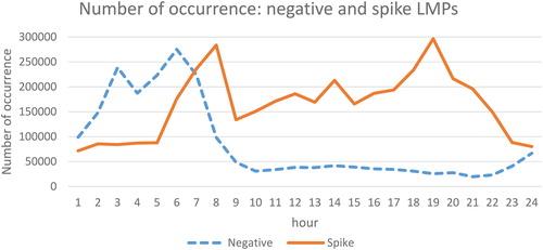
However, our results show that the efforts of the government do not significantly accomplish the foremost mission by reducing the occurrence of extreme prices in the electricity market. The emergence of renewable energy does not reduce the spike prices, but incurs the negative prices coexisted in the market. Figure 2 depicts the distribution of negative and spike LMPs in 24 hours. There is a reciprocal relationship between the numbers of negative and spike LMPs. However, the majority of negative LMPs appear between the midnight and the early morning during which the large amount of energy is definitely not needed. In the daytime and especially the working hours, the number of spike LMPs is far larger than the number of negative LMPs. Figure 2 confirms the dominant place of spike prices and the results from the PCA model. It further suggests that the current electricity market is still facing the shortage of energy, even after the adoption of renewable energy incentive mechanisms.

Figure 2. Distribution of negative and spike LMPs in one day.

Although the appearance of negative prices has limited power to reduce the over-demand situation and the accompanied spike prices, promoting the renewable energy is still a promising and meaningful policy for the long-term development of the electricity market. The NARDL model provides new insights from a new angle of view. Results of the NARDL model are from the overall market level rather than the regional level, and indicate that the negative prices have a significant effect to maintain the fluctuation of both the real-time market and the forward market. Developing diverse renewable energy will eventually the large demand and consequently facilitate the market price stability.

The concurrent production of renewable energy is tightly driven by the time-related factors. For example, the wind power is determined by the seasonality of wind, which makes the wind power fail to become a steady supplier. In addition, the limitations of transmission capacity are also a critical factor to cause the geographical energy imbalance. As the practical resolutions, the development of electrical energy storage (EES) can save the excessive energy during the over-supply period and release during the over-demand period. It may help reduce and remove the extreme prices in both types (Liu, Woo, & Zarnikau, 2017; Sioshansi et al., 2009). As another possible resolution, upgrading the transmission capacity may also help reduce the power inequilibrium. According to U.S. Energy Information Administration (2012a, 2012b), transmission loss and congestion are causes to incur the daily price fluctuations. Upgrading the transmission line can provide a smoother power transmission from over-supply regions to over-demand regions and consequently solve the spatial power inequilibrium.

5. Conclusion

As two frequently observed phenomena and the constituents of extreme values, spike and negative prices have opposite economic meanings. Negative prices indicate over-supply while spike prices indicate over-demand. This study assesses the impact of negative pricing and spike pricing on the price fluctuation. We evaluate the price fluctuation by the standard deviation of prices for each transmission line. We analyze the price data from the PJM electricity market including over 11,000 transmission lines with hourly updated records. For both negative and spike price groups, we calculate 16 relevant covariates by transmission lines. These covariates capture the distributions of spike prices and negative prices respectively.

To compare the effects on price fluctuations between negative prices and spike prices, we employ a two-stage analyses with a PCA model and a NARDL model. Through the result of PCA we select six components and interpret their implication related to the covariates. We find that components with the largest explanatory power to the variation of prices are highly related to spike LMPs and the position and the extent of concentration of the overall LMPs. Therefore, in the dimension of the individual transmission lines, there exists over-demand with a high frequency. Different from PCA, results of the NARDL model suggest that the negative prices have a larger potential effect on both the real-time market and the forward market. As an implication, our finding confirms the contribution of the renewable energy incentive mechanisms, and believes that the renewable energy will fulfill the energy demand and help balance the energy equilibrium in the future.

In summary, our results indicate that in the current electricity market, although types of renewable energy generators have already been participating and making contribution, the over-demand and energy shortage are still the big issues. The time-varying inequilibrium between power supply and demand are common in any area. From the perspective of policy makers, developing EES and upgrading the transmission capacity should be the resolution to reduce the market price fluctuations.

Additionally, our results suggest that PCA and NARDL are efficient tools for electricity market analyses. Using PCA, we can reduce the dimensionality of multivariate analysis, and discover the structural meaning of factors by constructing latent common structures. The NARDL model enables us to take a comprehensive picture of the overall market, and figure out the determinants of price fluctuations.

Acknowledgements

The authors thank Marinko Škare (Editor in Chief), Adriana Galant and Marijana Tadić (Editorial Assistants), and three anonymous referees. The authors also thank Carlo Andrea Bollino, Carlo Di Primio, Yalin Huang, Mengfei Jiang, Yu Jiang, Nasrin Khalili, David Knapp, Gürkan Kumbaroğlu, Desheng Lai, Alberto Lamadrid, Xi Liang, Hueichu (Ruby) Liao, Yun Liu, Fernando Navajas, Alberto Pincherle, Athanasios Pliousis, Michael Pollitt, Yunqiu Qiu, Gerardo Rabinovich, Anka Serbu, Nikolaos Thomaldis, Lan Wang, Nan Wang, Adonis Yatchew, participants at the 2018 Associazione Italiana Economisti dell’ Energia (AIEE) Energy Symposium, and 2019 Latin American Meeting of the Economy of Energy, for helpful comments and feedback.

Disclosure statement

The authors declare no conflict of interest.

Additional information

Funding

The authors gratefully acknowledge the support from National Natural Science Foundation of China (Grant No. 71803012), the Fundamental Research Funds for the Central Universities of China, and the Beijing Talents Fund of China (Grant No. 2016000020124G051).

References

- Aït-Sahalia, Y., & Xiu, D. (2019). Principal component analysis of high frequency data. Journal of the American Statistical Association, 114(525), 287–303.
- Bai, J. (2003). Inferential theory for factor models of large dimensions. Econometrica, 71(1), 135–171. doi:10.1111/1468-0262.00392
- Bai, J., & Ng, S. (2002). Determining the number of factors in approximate factor models. Econometrica, 70(1), 191–221. doi:10.1111/1468-0262.00273
- Baek, S., Cursio, J. D., & Cha, S. Y. (2015). Nonparametric factor analytic risk measurement in common stocks in financial firms: Evidence from Korean firms. Asia-Pacific Journal of Financial Studies, 44(4), 497–536. doi:10.1111/ajfs.12098
- Barbour, E. (2014). Can negative electricity prices encourage inefficient electrical energy storage devices? International Journal of Environmental Studies, 71(6), 862–876. doi:10.1080/00207233.2014.966968
- Baradar, M., & Hesamzadeh, M. R. (2014). Calculating negative LMPs from SOCP-OPF. Presented at Energy Conference (ENERGYCON), 2014 IEEE International IEEE, 1461–1466. doi:10.1109/ENERGYCON.2014.6850615
- Bessembinder, H., & Lemmon, M. (2002). Equilibrium pricing and optimal hedging in electricity forward markets. The Journal of Finance, 57(3), 1347–1382. doi:10.1111/1540-6261.00463
- Bilitewski, B. (2012). The circular economy and its risks. Waste Management, 32(1), 1–2. doi:10.1016/j.wasman.2011.10.004
- Cao, C., & Huang, J. (2007). Determinants of S&P 500 index option returns. Review of Derivatives Research, 10(1), 1–38. doi:10.1007/s11147-007-9015-5
- Carlton, D. W. (1977). Peak load pricing with stochastic demand. The American Economic Review, 67(5), 1006–1010.
- Chakrabarty, B., & Tyurin, K. (2011). Market liquidity, stock characteristics and order cancellations: The case of fleeting orders. Financial econometrics modeling: Market microstructure, factor models and financial risk measures (pp 33–66). Basingstoke, UK: Palgrave Macmillan.
- Crew, M. A., & Kleindorfer, P. R. (1976). Peak load pricing with a diverse technology. The Bell Journal of Economics, 7(1), 207–231. doi:10.2307/3003197
- Deng, L., Hobbs, B., & Renson, P. (2015). What is the cost of negative bidding by wind? A unit commitment analysis of cost and emissions. IEEE Transactions on Power Systems, 30(4), 1805–1814. doi:10.1109/TPWRS.2014.2356514
- Dutta, G., & Mitra, K. (2017). A literature review on dynamic pricing of electricity. Journal of the Operational Research Society, 68(10), 1131–1145. doi:10.1057/s41274-016-0149-4
- Engle, R., & Patton, A. (2001). What good is a volatility model? Quantitative Finance, 1(2), 237–245. https://doi.org/10.1016/B978-075066942-9.50004-2 doi:10.1088/1469-7688/1/2/305
- Forni, M., Hallin, M., Lippi, M., & Reichlin, L. (2000). The generalized dynamic-factor model: Identification and estimation. Review of Economics and Statistics, 82(4), 540–554. doi:10.1162/003465300559037
- Forni, M., Hallin, M., Lippi, M., & Reichlin, L. (2004). The generalized dynamic factor model: Consistency and rates. Journal of Econometrics, 119(2), 231–255. https://doi.org/10.1016/S0304-4076(03)00196-9 doi:10.1016/S0304-4076(03)00196-9
- Forni, M., & Lippi, M. (2001). The generalized dynamic factor model: Representation theory. Econometric Theory, 17, 1113–1141.
- Frömmel, M., Han, X., & Kratochvil, S. (2014). Modeling the daily electricity price volatility with realized measures. Energy Economics, 44, 492–502. doi:10.1016/j.eneco.2014.03.001
- Geman, H., & Roncoroni, A. (2006). Understanding the fine structure of electricity prices. The Journal of Business, 79(3), 1225–1261. doi:10.1086/500675
- Genoese, F., Genoese, M., & Wietschel, M. (2010). Occurrence of negative prices on the German spot market for electricity and their influence on balancing power markets. Paper presented at the Energy Market (EEM), 2010 7th International Conference on the European IEEE, 1–6.
- Hadsell, L., Marathe, A., & Shawky, H. A. (2004). Estimating the volatility of wholesale electricity spot prices in the US. The Energy Journal, 25(4), 23–40. doi:10.5547/ISSN0195-6574-EJ-Vol25-No4-2
- Hadsell, L., & Shawky, H. A. (2006). Electricity price volatility and the marginal cost of congestion: An empirical study of peak hours on the NYISO market, 2001-2004. The Energy Journal, 27(2), 157–179. doi:10.5547/ISSN0195-6574-EJ-Vol27-No2-9
- He, G., & Victor, D. G. (2017). Experiences and lessons from China’s success in providing electricity for all. Resources, Conservation and Recycling, 122, 335–338. doi:10.1016/j.resconrec.2017.03.011
- Holland, S., & Mansur, E. T. (2006). The short-run effects of time-varying prices in competitive electricity markets. Energy Journal, 27(4), 127–156.
- Ibrahim, M. H. (2015). Oil and food prices in Malaysia: A nonlinear ARDL analysis. Agricultural and Food Economics, 3(1), 2. doi:10.1186/s40100-014-0020-3
- Jammazi, R., Lahiani, A., & Nguyen, D. K. (2015). A wavelet-based nonlinear ARDL model for assessing the exchange rate pass-through to crude oil prices. Journal of International Financial Markets, Institutions and Money, 34, 173–187. doi:10.1016/j.intfin.2014.11.011
- Joskow, P., & Wolfram, C. (2012). Dynamic pricing of electricity. American Economic Review, 102(3), 381–385. doi:10.1257/aer.102.3.381
- Knittel, C. R., & Roberts, M. R. (2005). An empirical examination of restructured electricity prices. Energy Economics, 27(5), 791–817. doi:10.1016/j.eneco.2004.11.005
- Li, K., Cursio, J., & Sun, Y. (2018). Principal component analysis of price fluctuation in the smart grid electricity market. Sustainability, 10(11), 4019. doi:10.3390/su10114019
- Li, K., Cursio, J. D., Jiang, M., & Liang, X. (2019). The significance of calendar effects in the electricity market. Applied Energy, 235, 487–494. doi:10.1016/j.apenergy.2018.10.124
- Liu, Y., Woo, C.-K., & Zarnikau, J. (2017). Wind generation’s effect on the ex post variable profit of compressed air energy storage: Evidence from Texas. Journal of Energy Storage, 9, 25–39. doi:10.1016/j.est.2016.11.004
- Longstaff, F. A., & Wang, A. (2004). Electricity forward prices: A high-frequency empirical analysis. The Journal of Finance, 59(4), 1877–1900. doi:10.1111/j.1540-6261.2004.00682.x
- Nguyen, D. T. (1976). The problems of peak loads and inventories. The Bell Journal of Economics, 7(1), 242–248. doi:10.2307/3003199
- Nusair, S. A. (2017). The J-Curve phenomenon in European transition economies: A nonlinear ARDL approach. International Review of Applied Economics, 31(1), 1–27. doi:10.1080/02692171.2016.1214109
- Pesaran, M. H., Shin, Y., & Smith, R. J. (2001). Bounds testing approaches to the analysis of level relationships. Journal of applied econometrics, 16(3), 289–326. doi:10.1002/jae.616
- Seifert, J., & Uhrig-Homburg, M. (2007). Modelling jumps in electricity prices: Theory and empirical evidence. Review of Derivatives Research, 10(1), 59–85. doi:10.1007/s11147-007-9011-9
- Shin, Y., Yu, B., & Greenwood-Nimmo, M. (2013). Modelling asymmetric cointegration and dynamic multipliers in an ARDL framework. In W.C. Horrace & R.C. Sickles (Eds.), Festschrift in Honor of Peter Schmidt. New York (NY): Springer Science & Business Media.
- Simanaviciene, Z., Virgilijus, D., & Simanavicius, A. (2017). Psychological factors influence on energy efficiency in households. Oeconomia Copernicana, 8(4), 671–684. doi:10.24136/oc.v8i4.41
- Spees, K., & Lave, L. (2008). Impacts of responsive load in PJM: Load shifting and real time pricing. Energy Journal, 29(2), 101–122.
- Sioshansi, R., Denholm, P., Jenkin, T., & Weiss, J. (2009). Estimating the value of electricity storage in PJM: Arbitrage and some welfare effects. Energy Economics, 31(2), 269–277. doi:10.1016/j.eneco.2008.10.005
- Skiadopoulos, G., Hodges, S., & Clewlow, L. (2000). The dynamics of the S&P 500 implied volatility surface. Review of Derivatives Research, 3(3), 263–282. DOI doi:10.1023/A:1009642705121
- Stock, J. H., & Watson, M. W. (1998). Diffusion indexes. (Discussion paper). NBER.
- Stock, J. H., & Watson, M. W. (2002). Forecasting using principal components from a large number of predictors. Journal of the American Statistical Association, 97(460), 1167–1179. doi:10.1198/016214502388618960
- U.S. Energy Information Administration. (2012a). Negative prices in wholesale electricity markets indicate supply inflexibilities. Today in Energy.
- U.S. Energy Information Administration. (2012b). Negative wholesale electricity prices occur in RTOs. Today in Energy.
- Walawalkar, R., Blumsack, S., Apt, J., & Fernands, S. (2008). An economic welfare analysis of demand response in the PJM electricity market. Energy Policy, 36(10), 3692–3702. doi:10.1016/j.enpol.2008.06.036
- Wenders, J. T. (1976). Peak load pricing in the electric utility industry. The Bell Journal of Economics, 7(1), 232–241. doi:10.2307/3003198
- Xiao, Y., Colwell, D. B., & Bhar, R. (2015). Risk premium in electricity prices: Evidence from the PJM market. Journal of Futures Markets, 35(8), 776–793. doi:10.1002/fut.21681
- Yang, C. (2017). Opportunities and barriers to demand response in China. Resources, Conservation and Recycling, 121, 51–55. doi:10.1016/j.resconrec.2015.11.015
- Yuan, Z., Bi, J., & Moriguichi, Y. (2006). The circular economy: A new development strategy in China. Journal of Industrial Ecology, 10(1–2), 4–8. doi:10.1162/108819806775545321
- Zareipour, H., Bhattacharya, K., & Cañizares, C. A. (2007). Electricity market price volatility: The case of Ontario. Energy Policy, 35(9), 4739–4748. doi:10.1016/j.enpol.2007.04.006
- Zhao, Z., & Wu, L. (2014). Impacts of high penetration wind generation and demand response on LMPs in day-ahead market. IEEE Transactions on Smart Grid, 5(1), 220–229. pp doi:10.1109/TSG.2013.2274159
- Zhou, Y. (H.), Scheller-Wolf, A., Secomandi, N., & Smith, S. (2016). Electricity trading and negative prices: Storage vs. disposal. Management Science, 62(3), 880–898. doi:10.1287/mnsc.2015.2161