The role of housing sentiment in forecasting U.S. home sales growth: evidence from a Bayesian compressed vector autoregressive model

Abstract

Accurate forecasts of home sales can provide valuable information for not only policymakers, but also financial institutions and real estate professionals. Against this backdrop, the objective of our article is to analyse the role of consumers’ home buying attitudes in forecasting quarterly U.S. home sales growth. Our results show that the home sentiment index in standard classical and Minnesota prior-based Bayesian V.A.R.s fail to add to the forecasting accuracy of the growth of home sales derived from standard economic variables already included in the models. However, when shrinkage is achieved by compressing the data using a Bayesian compressed V.A.R. (instead of the parameters as in the B.V.A.R.), growth of U.S. home sales can be forecasted more accurately, with the housing market sentiment improving the accuracy of the forecasts relative to the information contained in economic variables only.

Keywords:

• home sales
• housing sentiment
• classical and Bayesian vector autoregressive models

JEL CLASSIFICATIONS:

• C32
• R31

1. Introduction

Academics suggest that housing market leads business cycles, and housing market activity affects the economy at both macroeconomic and microeconomic levels (Leamer, 2007, 2015).¹ Since housing represents a large share of the total economy, from a macroeconomic perspective, movements in the housing sector spills over to the entire economy through new constructions, renovations of existing property, and the volume of home sales. At the same time, at the microeconomic level, performances of financial institutions and real estate firms depend crucially on housing market activity, as suggested by the recent financial crisis. Hence, timely and accurate forecasts of home sales can provide valuable information to not only policymakers, but also to financial institutions and real estate professionals as well as housing market participants.

In spite of the importance of home sales, the literature (which we discuss below in detail) on forecasting home sales instead of house prices in the U.S. at the aggregate- and at regional levels is, however, as far as we know, limited to five studies (Dua & Miller, 1996; Dua, Miller, & Smyth, 1999; Dua & Smyth, 1995; Gupta, Tipoy, & Das, 2010; Hassani, Gupta, Ghodsi, & Segnon, 2017). These studies primarily rely on price of homes, mortgage rate, real personal disposable income, unemployment rate, building permits authorised, and housing starts as possible predictors that tend to affect home sales. This is understandable, since the first four factors capture the demand for housing, while the latter two affects the supply in the housing market. In this regard, it is important to point out that Dua and Smyth (1995) also studied the role of survey data on households’ buying attitudes for homes, but could not find an important role of this variable in forecasting home sales of the U.S. economy.

More recently however, i.e., in the wake of the ‘Great Recession’ which is now very well knwn to have been caused by the collapse of the housing market (Gupta, Lv, & Wong, 2019), Case, Shiller, and Thompson (2012, 2014) have argued that it is important to consider people’s opinions about buying conditions, also referred to as housing sentiment, in analysing housing market decisions. The intuition is that housing sentiment captures the expectation of economic agents regarding how the housing market is going to behave in the future, and hence, from a behavioural perspective, act as a determinant of home purchase decisions, either for consumption or investment via renting it out. Against this backdrop, the objective of our article is to revisit the role of including consumers’ home buying attitudes (besides the above-mentioned demand–supply predictors) in forecasting home sales growth of the U.S., which has been earlier suggested to be of no importance by Dua and Smyth (1995). In general, the main obstacle in analysing the impact of people’s opinions about buying conditions on housing market movements and comparing this to other competing predictors is usually the lack of a quantifiable metric of housing sentiment measured consistently over a sufficiently long period to implement a proper forecasting exercise. In this context, the above problem has been solved recently by Bork, Møller, & Pedersen (forthcoming), who has constructed a news housing market sentiment index based on household responses to questions regarding house buying conditions from the consumer survey of the University of Michigan. Bork et al. (forthcoming) showed that the housing sentiment explains a large share of the time-variation in house prices during both boom and bust cycles and it strongly outperforms several macroeconomic variables typically used to forecast house prices.² Given this, we forecast quarterly U.S. home sales, over an out-of-sample period of 1995:1 to 2014:3, by using an in-sample training period of 1975:3 to 1994:4, by using this broad housing sentiment index, over and above the standard predictors used in the literature. By comparing our econometric models with and without the housing market sentiment variable, we are able to evaluate the role played by home buying attitudes of consumers in forecasting home sales growth of the U.S.

Regarding our econometric framework, just like the existing studies (which we discuss in detail in Section 2), we rely on both classical and Bayesian V.A.R. models for analysing the ability of housing sentiment in forecasting home sales of the U.S. economy. However, unlike the literature on home sales forecasting using B.V.A.R.s, which imposes the popular Minnesota prior shrinkage on the parameters to overcome issues of over-parameterisation in classical V.A.R.s (resulting in the favourable performance of the former), we use a Bayesian Compressed V.A.R. (B.C.V.A.R.) framework. In the B.C.V.A.R. model, shrinkage is achieved by compressing the data instead of the parameters. A crucial aspect of this method is that the projections used to compress the data are drawn randomly in a data oblivious manner. Then, through Bayesian model averaging (B.M.A.), different weights are assigned to the projections where the weights are determined according to the explanatory power of the compressed variables on the dependent variable. In other words, the projections do not involve the data, and thus, compute trivially, which is not often the case with B.V.A.R. models based on priors other than the Minnesota prior. To the best of our knowledge, this is the first article to forecast U.S. home sales by using a B.C.V.A.R. model, based on a housing sentiment index, which summarises a broader set of information on consumers’ home buying attitudes. In the process, our article aims to analyse the role of both a new measure of housing sentiment and a new econometric framework in forecasting home sales, and hence add to the literature in two dimensions, i.e., methodology and the predictor-set.

The remainder of the article is organised as follows: Section 2 presents the literature review, while Section 3 lays out the basics of the econometric models used, and Section 4 discusses the data and results, with Section 5 concluding the article.

2. Literature review

As indicated above, the literature on forecasting home sales in the U.S. at the aggregate and at regional levels is limited to five studies, namely, Dua and Smyth (1995), Dua and Miller (1996), Dua et al. (1999), Gupta et al. (2010), and Hassani et al. (2017). While Dua and Smyth (1995) used Bayesian V.A.R. (B.V.A.R.) models to forecast home sales for the aggregate U.S. economy, Dua and Miller (1996) extended the models from Dua and Smyth (1995) to forecast home sales for the state of Connecticut. In their original model, Dua and Smyth (1995) considered home sales, price of homes, mortgage interest rate, real disposable income, unemployment rate, as well as, survey data on households' buying attitudes for homes. However, the authors showed that, the gain from including the survey data in the model is small because the efforts have been included in other economic variables.³ Dua and Miller (1996) extended the benchmark model (containing home sales, price of homes, mortgage interest rate, real disposable income, and unemployment rate) of Dua and Smyth (1995), by including a leading index for the Connecticut economy. They showed that, by doing so, one can improve the forecast performance of the benchmark model substantially. Given this result, Dua et al. (1999) extended the model described in Dua and Smyth (1995) by adding six different leading indicators, namely housing permits authorised, housing starts, the U.S. Department of Commerce’s composite index of eleven leading indicators, the short- and long-leading indices developed by the Center for International Business Cycle Research (C.I.B.C.R.) at Columbia University, and the leading index constructed by C.I.B.C.R. that focused solely on employment related variables. They found that the benchmark B.V.A.R. model (which included, as before, home sales, price of homes, mortgage rate, real personal disposable income, and unemployment rate) supplemented by the building permits authorised as the leading indicator consistently produced the most accurate forecasts. In addition, Dua et al. (1999) noted that replacing building permits with housing starts generated equally accurate forecasts of home sales. Gupta et al. (2010) analysed the ability of a wide array of forecasting models, which included classical and Bayesian vector–error correction (V.E.C.) models, besides the random walk (R.W.), the autoregressive (A.R.), and B.V.A.R. models, in forecasting home sales for the four U.S. census regions (Northeast, Midwest, South, West). In their analysis, Gupta et al. (2010) used home sales, price of homes, mortgage rate, real personal disposable income, unemployment rate, and building permits authorised, i.e., the model prescribed by Dua et al. (1999). This study found that except for the South-region, the Bayesian type models outperformed all the other models in forecasting home sales at all forecasting horizons, and were also capable of predicting the peaks and declines in home sales with tremendous accuracy. In sum, the general consensus is that the Bayesian type models are better equipped in forecasting home sales than their classical counterparts.

More recently, Hassani et al. (2017) build on this line of literature, by comparing the ability of two different versions of Singular Spectrum Analysis (S.S.A.) methods, namely, Recurrent S.S.A. (R.S.S.A.) and Vector SSA (V.S.S.A.), in univariate and multivariate frameworks, in forecasting seasonally unadjusted home sales for the aggregate U.S. economy and its four census regions. Given the dominance of V.A.R. models in the home sales forecasting literature, Hassani et al. (2017) compared the performance of the S.S.A.-based models with classical and Bayesian variants of the autoregressive and vector autoregressive models. The authors found that the univariate V.S.S.A. was the best performing model for the aggregate U.S. home sales, while the multivariate versions of the R.S.S.A. was the outright winner in forecasting home sales for all the four census regions. In the process, their results highlighted the superiority of the nonparametric S.S.A. approach.

In sum, the literature has relied on traditional demand and supply factors in forecasting aggregate and regional home sales of the U.S. economy, primarily based on V.A.R. type models. Dua and Smyth (1995) is the only study to have considered housing sentiment, while Hassani et al. (2017) also investigated an alternative econometric framework based on S.S.A. While Dua and Smyth (1995) suggested a weak role for housing sentiment nearly two and half-decades back, the recent emphasis of sentiments-related variable in the wake of the global financial crisis by Case et al. (2012, 2014) in affecting housing market decisions, provide us with the motivation to revisit the role of consumer’s home buying attitudes in forecasting home sales growth, based on an improved measure of housing sentiment as developed by Bork et al. (forthcoming). Understandably, the decision to do so is due to the fact that the U.S. economy, and the housing sector in general have undergone tremendous evolution post-2007, i.e., the recent crisis. In addition, we are also able to investigate our question, based on recent developments of econometric methodologies in the context of B.V.A.R.s, than those used in the existing literature. In essence, our analysis is an application of recent econometric methodology associated with B.V.A.R.s in analysing the predictive content of a broad measure of housing market sentiment in forecasting home sales growth of the U.S. economy based on updated information derived from recent data that covers the global financial crisis.

3. Methodology

Following Koop, Korobilis, and Pettenuzzo (2019), we use the following framework based on the B.C.V.A.R. model, as our main focus, by starting off from the basic formulation of a V.A.R. model: (1) $$Y_t={\beta Y}_{t-1}+{\epsilon }_t$$(1) where $Y_t$ (t = 1,…,T) represents an n$\times$1 vector containing observations on n time 1 series of variables, ${ϵ}_t$ is i.i.d. $N(0, \mathrm{\Omega })$ and $\beta$ is an n$\times$n matrix of coefficients. Under the classical V.A.R. model, no restrictions are imposed on the β-matrix of the coefficients, i.e., they are left unrestricted. Due to issues of overparameterisation in V.A.R. models resulting in multicollinearity and a loss of degrees of freedom leads to inefficient estimates and possibly large out-of-sample forecasting errors, we next discuss the compression of the data. In order to compress the explanatory variables in the V.A.R., we can use the projection matrix $\mathrm{\Phi }$ as described in Koop et al. (2019), where Φ is a m$\times$k matrix drawn from the following distribution: $$\mathrm{Pr}\left({\varphi }_{\mathit{ij}}=\frac{1}{\sqrt{\phi }}\right)={\phi }^2$$ (2) $$\mathrm{Pr}\left({\varphi }_{\mathit{ij}}=0\right)=2(1-\phi )\mathrm{ }\phi ,$$(2) $$\mathrm{Pr}\left({\varphi }_{\mathit{ij}}=\frac{1}{\sqrt{\phi }}\right){=(1-\phi )}^2$$ where $\phi$ and $m$ are unknown parameters. Next, they rely on B.M.A. to average across the different random projections. Treating each ${\Phi }^r$(r = 1,…., R) as defining a new model, we first calculate the marginal likelihood for each model. Thereafter, we average across the various models by using weights proportional to the marginal likelihoods. We also note that both m and $\phi$ can be estimated as part of the B.M.A. exercise. With the estimated projection matrix, we can compress the explanatory variables in the V.A.R. and define the compressed V.A.R. model as follows: (3) $$Y_t={{\beta }^c(\mathrm{\Phi }Y}_{t-1})+{\epsilon }_t,$$(3)

subjected to the normalisation ${\mathrm{\Phi }}^{\prime }\mathrm{\Phi }=\mathrm{\iota }$. Finally, the full predictive density $p(\left.Y_{t+h}\right|M_r{D}^t)$ (i.e., M₁,…,M_R) is obtained for each compressed V.A.R. model by using the predictive simulation method as descripted in Koop et al. (2019). Therefore, the final B.M.A. forecast for each forecast at horizon h can be represented as: (4) $$\mathrm{p}\left(\left.Y_{t+h}\right|D^t\right)=\sum _{r=1}^R{\omega }_r\mathrm{p}\left(\left.Y_{t+h}\right|{M_r,D}^t\right),$$(4) where $D^t$ is the information set available at time t, ${\omega }_r=\exp \left(-.5{\mathrm{\Psi }}_r\right)/{\sum }_{r=1}^R\exp (-.5{\mathrm{\Psi }}_r)$ is the model $M_r$ weight, and ${\mathrm{\Psi }}_r={\mathit{BIC}}_r-{\mathit{BIC}}_{\mathit{min}}$, with ${\mathit{BIC}}_r$ be the value of the Bayesian Information Criterion (B.I.C.) of model $M_r$ and ${\mathit{BIC}}_{\mathit{min}}$ be the minimum value of the B.I.C. among all R models.

Besides the B.C.V.A.R., we also estimate the standard classical V.A.R. and B.V.A.R. models, with the latter based on the popular Minnesota-prior shrinkage on the parameters of the model, by imposing restrictions on these coefficients based on the assumption that they are more likely to be near zero than the coefficients on shorter lags. However, if there are strong effects from less important variables, the data can override this assumption. The restrictions are imposed by specifying normal prior distributions with zero means and small standard deviations for all coefficients with the standard deviation decreasing as the lags increase. The exception to this is, however, the coefficient on the first own lag of a variable, which has a mean of unity, but is also set to zero if the variables in the B.V.A.R. are mean-reverting (as in our case).⁴ Our implementation of the B.V.A.R., which involves a single prior shrinkage parameter (ω), follows closely the approach used by Banbura et al. (2010). However, different from Banbura et al. (2015), we modify the approach by following Giannone, Lenza, and Primiceri (2015) to estimate ω in a data-based fashion. As in Koop et al. (2019), we choose a grid of values for the inverse of the shrinkage factor ω⁻¹ ranging from 0.5$\times \sqrt{\mathit{np}}$ to 10$\times \sqrt{\mathit{np}}$, in increments of 0.1$\times \sqrt{\mathit{np}}$. At each point in time, the B.I.C. is used to choose the optimal degree of shrinkage. All remaining specification and forecasting choices are exactly the same as in Banbura, Giannone, and Reichlin (2010), and hence, we skip reporting the procedure.

Note that, our article aims to apply the B.C.V.A.R. approach to forecasting home sales growth based on information of housing market sentiment (after controlling for price of homes, mortgage rate, real personal disposable income, unemployment rate, building permits authorised, and housing starts), while Koop et al. (2019) used the framework to forecast seven major macroeconomic variables of the U.S. economy (namely, industrial production growth, the unemployment rate, total nonfarm employment, the change in the Fed funds rate, the change in the 10 year T-bill rate, the finished good producer price inflation and consumer price inflation), based on a small-, medium- and large-scales B.C.V.A.R.s comprising of seven, 19 and 129 macroeconomic variables respectively, that is available from the F.R.E.D.-M.D. database (McCracken & Ng, 2016).

4. Data and results

As discussed in the introduction, our data set covers the quarterly period of 1975:3 to 2014:3, with the start and end date being purely driven by the availability of the housing sentiment index developed by Bork et al. (forthcoming). The authors use time series data from the consumer surveys of the University of Michigan to generate the housing sentiment index, with housing sentiment defined based on the general attitude of households about house buying conditions. In particular, Bork et al. (forthcoming) consider the underlying reasons households to provide their views about all the house buying conditions. The part of University of Michigan’s consumer survey related to house buying conditions starts with the question: ‘Generally speaking, do you think now is a good time or a bad time to buy a house?’, with the follow-up question: ‘Why do you say so?’ In constructing the index, Bork et al. (forthcoming) focused on the responses to the follow-up question as the idea is to draw on the information in the underlying reasons why households believe that it is a bad or good time to buy a house. Specifically, the housing sentiment index is based on the following 10 time series: good time to buy; prices are low, good time to buy; prices are going higher, good time to buy; interest rates are low, good time to buy; borrow-in-advance of rising interest rates, good time to buy; good investment, good time to buy; times are good, bad time to buy; prices are high, bad time to buy; interest rates are high, bad time to buy; cannot afford, and bad time to buy; uncertain future. Then Bork et al. (forthcoming) used partial least squares (P.L.S.) to aggregate the information contained in each of the 10 time series into an easy-to-interpret index of housing sentiment, with P.L.S. filtering out idiosyncratic noise from the individual time series and summarising the most important information in a single index.⁵

Besides using the index measuring consumers’ home buying attitudes capturing housing market sentiment, the other variables used include: sales of new and single-family houses, median sale prices of new and single-family houses, 30-year conventional mortgage rate, real disposable personal income (in chained 2009 dollars), civilian unemployment rate, new private housing units authorised by building permits, and new privately owned housing units started. Note that, on one hand, the price of homes, income, interest rate, unemployment rate, would all determine the ability of economic agents to buy a property either for consumption or investment. In other words, these variables capture the demand for housing. Housing starts and permits on the other hand, is a leading indication of the supply of housing in the market. Taken together, these six variables, capture demand- and supply-sides of the economy. Data on home sales and prices are obtained from the Census Bureau of the U.S., while the other variables are derived from the F.R.E.D. database of the Federal Reserve Bank of St. Louis. All the variables are seasonally adjusted, and are converted into quarterly data based on temporal aggregation when it is available at a higher frequency. Following Koop et al. (2019), we ensure that all variables are approximately mean-reverting which, in turn, requires us to use growth rates of home sales and prices, and that of real disposable personal income. In the Appendix of the article, Figure A1 plots the eight variables of our concern while Table A1 provides the summary statistics for the variables.

To avoid forward-looking bias, we follow Bork et al. (forthcoming) to compute the housing sentiment index in a recursive manner over 1995:1–2014:3. Thereafter, we use the same time-frame as the out-of-sample period in our forecasting exercise, with our models being estimated recursively over this period as well producing one- to twelve-quarters-ahead forecasts. The lag-length chosen for the V.A.R. models is 1, based on the B.I.C.

For our forecasting, we estimate two-versions each of the classical V.A.R. model, B.V.A.R. model and the B.C.V.A.R. model. In the first case of each of the V.A.R., B.V.A.R. and B.C.V.A.R. models, we include home sales, price of homes, mortgage rate, real personal disposable income, unemployment rate, building permits authorised, and housing starts. Building on the results of the first model, we incorporate the housing sentiment index in the second version of the V.A.R., B.V.A.R. and B.C.V.A.R. models, along with all the previously-mentioned variables. Hence, we end up with six models, three for each case. We then compare the mean squared forecast errors (M.S.F.E.s) from each of the models, relative to the M.S.F.E. of the naïve (no-change) forecasting model, which we call the relative M.S.F.E. (R.M.S.F.E.). Understandably, a R.M.S.F.E. value of less (greater) than one, would suggest that the particular model analysed performs better (worse) than the naïve model. The R.M.S.F.E. for each model is reported in Table 1 for forecasting horizons 1 to 12, along with the average values of the same, over all these forecasting horizons – a metric that has been used widely in the abovementioned home sales forecasting literature to decide on the optimal (best-performing) forecasting model.

Table 1. Forecasting Performance of Alternative V.A.R. Models.

	Forecasting Models
Forecast Horizon (h)	VAR1	BVAR1	BCVAR1	VAR2	BVAR2	BCVAR2
1	0.4952	0.4888	0.0267	0.4916	0.4918	0.0288
2	0.3601	0.3464	0.0973	0.3560	0.3503	0.2108
3	0.5321	0.5013	0.0492	0.5425	0.5091	0.1198
4	2.6433	2.4992	0.4672	2.6806	2.5129	0.4641
5	0.5169	0.4836	0.0084	0.5043	0.4827	0.0034
6	0.3425	0.3241	0.4360	0.3368	0.3247	0.6161
7	0.5373	0.5170	0.0648	0.5366	0.5181	0.1503
8	1.9184	1.8736	5.4171	1.9344	1.8746	4.5827
9	0.4724	0.4637	0.1558	0.4668	0.4622	0.2324
10	0.3108	0.3098	0.0000	0.3055	0.3091	0.0097
11	0.4736	0.4809	0.0202	0.4683	0.4793	0.0628
12	1.7479	1.7846	0.6859	1.7373	1.7780	0.4464
Average	0.8625	0.8394	0.6191	0.8634	0.8411	0.5773

Note: Entries are relative mean square forecast errors of a specific model against the naïve (random walk) model (R.M.S.F.E.); V.A.R.1 (V.A.R.2), B.V.A.R.1 (B.V.A.R.2), and B.C.V.A.R.1 (B.C.V.A.R.2) represent the typical V.A.R. without housing sentiment (with housing sentiment included), the Bayesian V.A.R. based on the Minnesota prior without housing sentiment (with housing sentiment included), and the Bayesian compressed V.A.R. without housing sentiment (with housing sentiment included); Bold entries indicate when the model performs the best in terms of the R.M.S.F.E.; For h = 8, the naïve model performs the best.

We can make the following observations from Table 1: (1) The various V.A.R.s considered consistently outperform the naïve model for all horizons, with the exception of eight-, and 12-quarters-ahead forecasts. At horizon h = 8, the naïve model performs better than all the V.A.R. models, while at h = 12, the same holds true relative to the V.A.R.s and the B.V.A.R.s, but not the B.C.V.A.R.s; (2) On average, adding information of the housing sentiment index does not have any value added to forecasting accuracy of home sales growth derived from the V.A.R. and B.V.A.R. models. This result is consistent with that of Dua and Smyth (1995); (3) Based on the average value of the R.M.S.F.E., the B.V.A.R. models outperform their corresponding classical counterparts, but the B.C.V.A.R. models performs better than both V.A.R. and B.V.A.R. models; (4) Within the B.C.V.A.R. models, the B.C.V.A.R.2 model outperforms the B.C.V.A.R.1 model based on the average R.M.S.F.E., producing a gain of 6.7457 percent⁶ and; (5) If we look at the individual forecasting horizon, the best performing model at each horizon, based on the lowest M.S.F.E. (as shown by the bold entries in each row) across each models are as follows: For horizons, 1, 2, 3, 7, 9, 10 and 11, the B.C.V.A.R.1 is the outright favourite, while B.C.V.A.R.2 does the best at horizons 4,5 and 12. For the remaining two horizons, B.V.A.R.1 wins the race at horizon 6, and surprisingly the naïve model at the horizon 8.

In sum, we observe that shrinkage or either parameters (i.e., B.V.A.R.s) or data (B.C.V.A.R.s) matter in terms of outperforming the classical V.A.R. which has no restrictions imposed. Within the class of the Bayesian versions of the V.A.R., when shrinkage is achieved by compressing the data (as done in the B.C.V.A.R.s) instead of the parameters (as implemented in the B.V.A.R.s), growth of U.S. home sales can be forecasted relatively more accurately. In other words in the B.C.V.A.R.s, when a big dimensional problem is turned into a smaller, more computationally tractable one, with B.M.A. done over various compressions by attaching greater weight to compressions, we obtain more accurate forecast of home sales growth of the aggregate U.S. economy. This result highlights the first contribution of our application in the sense that we show that by applying a different type of more recent Bayesian approach based on data compression (i.e., the B.C.V.A.R.), unlike what has been previously done in the literature with shrinkage based on parameters (B.V.A.R.), we can obtain better results for home sales predictability. In addition, in this (B.C.V.A.R.) framework, the housing market sentiment tends to improve the accuracy of the forecasts for home sales growth, when compared to the information contained in economic variables only aiming to capture demand–supply conditions of the housing market. This result in turn, is the second contribution of our article, as it shows that housing market sentiment brings in additional behavioural information beyond the information contained in standard variables that have been used in the literature of home sale forecasting of the U.S. economy thus far. This result confirms the suggestions of Case et al. (2012, 2014), who emphasise the need to incorporate housing market sentiment in the wake of the recent financial crisis, which originated from the housing market, to capture the expectations of agents about how the housing market is going to behave in the future. Housing sentiment affects the consumption and investment decisions of housing market participants and hence, shapes the future path of home sales.⁷

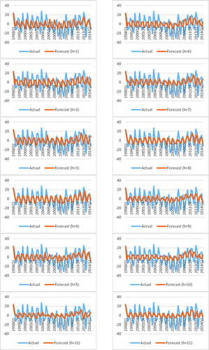
In Figure 1, we plot the forecasts at various horizons generated from the B.C.A.V.R.2 model, i.e., the Bayesian Compressed V.A.R. with the sentiment included, as it is the ‘optimal’ model, on average over the 12-quarters considered, along with the actual values of the home sales growth.⁸ As can be seen from the Figure, the B.C.V.A.R.2 model does quite well in predicting the turning points in the data by moving in the same direction as the actual values of home sales growth, but the forecasts are relatively less volatile than the actual data.

Figure 1. Actual versus Forecasts from B.C.V.A.R.2 Model.

Note: See Notes to Table 1.

5. Conclusion

The housing market activity in the U.S. has been shown to affect the economy at both the macroeconomic and the microeconomic level. Hence, timely and accurate forecasts of home sales can provide valuable information not only, for policymakers, but also for housing market participants (financial institutions and real estate professionals). Given this, we analyse the role of including consumers’ home buying attitudes, in a model that contains information on lagged economic variables (such as, price of homes, mortgage rate, real personal disposable income, unemployment rate, building permits authorised and housing starts, besides home sales itself), for forecasting quarterly U.S. home sales, over an out-of-sample period of 1995:1 to 2014:3. In doing so, we rely on both classical and Bayesian V.A.R. models for analysing the ability of a newly developed broad housing sentiment index in forecasting growth of home sales of the U.S. economy. Besides using the popular Minnesota prior shrinkage on the parameters to overcome issues of over-parameterisation in classical VARs, we also consider a B.C.V.A.R. model. In the B.C.V.A.R. model, shrinkage is achieved by compressing the data instead of the parameters. Our results show that, when shrinkage is achieved by compressing the data instead of the parameters, the growth rate of U.S. home sales can be forecasted more accurately. In addition, the housing market sentiment capturing consumers’ home buying attitudes, included in the B.C.V.A.R. model, tends to improve the accuracy of the forecasts for home sales growth, when compared to the information contained in economic variables only. This model also tends to predict well the turning points of the home sales growth. Our results thus highlight the importance of compressing the data over the parameters in Bayesian models, when forecasting home sales based on housing sentiment, over and above standard economic variables.

As indicated earlier, movements in the housing sector spills over to the entire economy through new constructions, renovations of existing property, and the volume of home sales. In addition, performances of financial institutions and real estate firms depend crucially on housing market activity. Hence, timely and accurate forecasts of home sales can provide valuable information to not only policymakers, but also to financial institutions and real estate professionals as well as housing market participants. Given these issues, our analysis have important implications for these economic agents. In particular, our results point out that market participants and policymakers can benefit by including housing market sentiment, besides standard demand–supply predictors, when forecasting home sales. Accurate forecasting of home sales would give an indication to policymakers as to whether the economy is heading for an expansion or recession, and help in the design of appropriate monetary and fiscal policies to ensure stability in the macroeconomy. Recall, policies take time to impact the economy, hence, forecasting the future path of the economy based on accurate predictions of home sales is of tremendous importance to policy authorities. In addition, financial market participants, can make projections about future profitability of their firms based on the prediction of home sales. But agents in the economy must realise that they would need to incorporate behavioural information to get more accurate forecasts home sales, rather than just relying on standard demand–supply factors. Furthermore, these agents must also understand that forecasts from standard methods traditionally used can be improved further by using recent advances in econometric models, which in turn involves compressing the data, rather than the parameter space.

Given that Bork et al. (forthcoming) has shown that the national housing sentiment index can also accurately forecast regional housing price growth rates, as part of future research, it would be interesting to check, whether the same hold for regional home sales growth rates as well.

Acknowledgements

We would like to thank three anonymous referees for many helpful comments. However, any remaining errors are solely ours.

Disclosure statement

No potential conflict of interest was reported by the authors.

Notes

1 Large number of studies has reported a strong link between the housing market and the economic activity in the U.S. (see for example Aye et al. (2014), Nyakabawo et al. (2015), and Emirmahmutoglu et al. (2016) for detailed literature reviews in this regard).

2 In-sample evidence, in this regard, can also be found in Dua (2008).

3 Interestingly, recent papers by Baghestani, Kaya, and Kherfi (2013) and Baghestani (2017) have highlighted the role of consumers’ home buying attitudes in predicting in-sample movements of U.S. home sales, while, the importance of financial variables (Federal funds rate, mortgage rate, and term-spread) in doing the same has been stressed by Baghestani and Kaya (2016). But, it is well-known that in-sample predictability does not necessarily translate into out-of-sample forecasting gains, with Campbell (2008) pointing out that, the ultimate test of any predictive model is its out-of-sample performance. However, this positive result in favour of consumers' home buying attitudes (as well as financial variables) in predicting home sales could be a result of the fact that the models used in these studies are only bivariate in nature, consisting of home sales and consumers' home buying attitudes or financial variables.

4 Based on the suggestion of an anonymous referee, we also imposed the sum-of-coefficients and dummy-initial-observation priors, as in Giannone et al. (2015). However, the performances of these B.V.A.R. models, i.e., sum-of-coefficients and dummy-initial-observation priors, were virtually similar to that of the model with the Minnesota prior, with average R.M.S.F.E. being 1.0005 and 1.0000 respectively. Given this, we have suppressed these results to save space, but are available upon request from the authors.

5 The data is available for download from: https://www.dropbox.com/s/al3sddq1026xci2/Online%20data.xlsx?dl=0.

6 Based on the suggestion of an anonymous referee, we also estimated an Artificial Neural Network (A.N.N.) model. We found that, on average, the A.N.N. model performed way worse, with the R.M.S.F.E. between the A.N.N. and B.C.V.A.R.2 being 56.20. Given that the literature on home sales forecasting has primarily concentrated on V.A.R.-type models, these results have been suppressed to save space, but are available upon request from the authors.

7 However, it is also important to qualify this statement a bit. If we compare the forecasting performance of the B.C.V.A.R.1 with that of the B.C.V.A.R.2 model by leaving out h = 8, where both these models perform poorly relative to the naïve model (with B.C.V.A.R.1 performing worst amongst all the models), then the former ends up being the preferred model, with an average R.M.S.F.E. of 0.1829 compared to 0.2132.

8 All forecast plots start from the common period of 1998:Q1 to correspond with the 12-steps-ahead forecasts.

Appendix

Figure A1. Data plot.

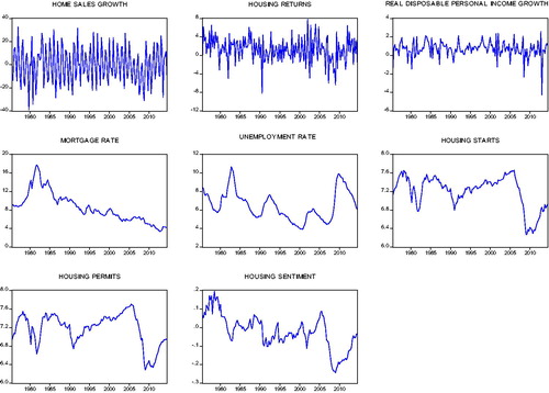
Table A1. Summary statistics.

	Variable
Statistic	HOME SALES GROWTH	HOUSING RETURNS	REAL DISPOSABLE PERSONAL INCOME GROWTH	MORTGAGE RATE	UNEMPLOYMENT RATE	HOUSING STARTS	HOUSING PERMITS	HOUSING SENTIMENT
Mean	−0.2583	1.2529	0.6856	8.5151	6.5057	7.2035	7.1766	−0.0231
Median	−0.6557	1.2679	0.7169	8.0100	6.1333	7.2971	7.2572	−0.0263
Maximum	32.5054	7.7731	2.5925	17.7333	10.6667	7.6593	7.7090	0.1958
Minimum	−38.9961	−8.1952	−4.2652	3.3600	3.9000	6.2647	6.2891	−0.2441
Std. Dev.	15.8673	2.7665	0.8764	3.2005	1.5766	0.3454	0.3369	0.0910
Skewness	−0.0052	−0.3538	−1.4574	0.7933	0.5420	−1.1086	−0.8899	−0.1816
Kurtosis	2.1780	3.4672	9.4030	3.2773	2.6277	3.5104	3.1166	3.0846
Jarque-Bera	4.4211	4.7038	323.7811	16.9697	8.5935	33.8597	20.8111	0.9093
Probability	0.1096	0.0952	0.0000	0.0002	0.0136	0.0000	0.0000	0.6347
Observations	157

Note: Std. Dev. stands for standard deviation, while probability is the p-value for the Jarque-Bera test, with the null hypothesis of normality.

References

- Aye, G. C., Balcilar, M., Bosch, A., & Gupta, R. (2014). Housing and the business cycle in South Africa. Journal of Policy Modeling, 36(3), 471–491. doi: 10.1016/j.jpolmod.2014.03.001
- Baghestani, H. (2017). Do consumers’ home buying attitudes explain the behaviour of US home sales? Applied Economics Letters, 24(11), 779–783. doi: 10.1080/13504851.2016.1229401
- Baghestani, H., & Kaya, I. (2016). Do financial indicators have directional predictability for US home sales? Applied Economics, 48(15), 1349–1360. doi: 10.1080/00036846.2015.1100253
- Baghestani, H., Kaya, I., & Kherfi, S. (2013). Do changes in consumers’ home buying attitudes predict directional change in home sales? Applied Economics Letters, 20(5), 411–415. doi: 10.1080/13504851.2012.709597
- Banbura, M., Giannone, D., & Reichlin, L. (2010). Large Bayesian vector autoregressions. Journal of Applied Econometrics, 25, 71–92. doi: 10.1002/jae.1137
- Bork, L., Møller, S. V., & Pedersen, T. Q. (2019). A new index of housing sentiment. Management Science. doi: 10.1287/mnsc.2018.3258
- Campbell, J. Y. (2008). Viewpoint: Estimating the equity premium. Canadian Journal of Economics/Revue Canadienne D’économique, 41(1), 1–21. doi: 10.1111/j.1365-2966.2008.00453.x
- Case, K. E., Shiller, R. J., & Thompson, A. K. (2012). What have they been thinking? Home buyer behavior in hot and cold markets. Brookings Papers on Economic Activity, 45(2), 265–315. doi: 10.1353/eca.2012.0014
- Case, K. E., Shiller, R. J., & Thompson, A. K. (2014). What have they been thinking? Home buyer behavior in hot and cold markets–a 2014 update. Cowles Foundation Discussion Paper, No. 1876R.
- Dua, P. (2008). Analysis of consumers’ perceptions of buying conditions for houses. The Journal of Real Estate Finance and Economics, 37(4), 335–350. doi: 10.1007/s11146-007-9084-0
- Dua, P., & Miller, S. M. (1996). Forecasting Connecticut home sales in a BVAR framework using coincident and leading indexes. Journal of Real Estate Finance and Economics, 13(3), 219–235.
- Dua, P., Miller, S. M., & Smyth, D. J. (1999). Using leading indicators to forecast US home sales in Bayesian VAR framework. The Journal of Real Estate Finance and Economics, 18(2), 191–205. doi: 10.1023/A:1007718725609
- Dua, P., & Smyth, D. J. (1995). Forecasting U.S. home sales using BVAR models and survey data on households’ buying attitudes for homes. Journal of Forecasting, 14(3), 167–180. doi: 10.1002/for.3980140306
- Emirmahmutoglu, F., Balcilar, M., Apergis, N., Simo-Kengne, B. D., Chang, T., & Gupta, R. (2016). Causal relationship between asset prices and output in the US: Evidence from state-level panel Granger causality test. Regional Studies, 50(10), 1728–1741. doi: 10.1080/00343404.2015.1055462
- Giannone, D., Lenza, M., & Primiceri, G. (2015). Prior selection for vector autoregressions. Review of Economics and Statistics, 97(2), 436–451. doi: 10.1162/REST_a_00483
- Gupta, R., Lv, Z., & Wong, W.-K. (2019). Macroeconomic shocks and changing dynamics of the U.S. REITs sector. Sustainability, 11(10), 2776. doi: 10.3390/su11102776
- Gupta, R., Tipoy, C. K., & Das, S. (2010). Could we have predicted the recent downturn in home sales of the four US census regions? Journal of Housing Research, 19(2), 111–128.
- Hassani, H., Gupta, R., Ghodsi, Z., & Segnon, M. K. (2017). Forecasting home sales in the four census regions and the aggregate US economy using singular spectrum analysis. Computational Economics, 49(1), 83–97. doi: 10.1007/s10614-015-9548-x
- Koop, G., Korobilis, D., & Pettenuzzo, D. (2019). Bayesian compressed vector autoregressions. Journal of Econometrics, 201, 135–154. doi: 10.1016/j.jeconom.2018.11.009
- Leamer, E. E. (2007). Housing is the business cycle. Proceedings - Economic Policy Symposium - Jackson Hole, Federal Reserve Bank of Kansas City, pp. 149–233.
- Leamer, E. E. (2015). Housing really is the business cycle: What survives the lessons of 2008-09? Journal of Money, Credit and Banking, 47(S1), 43–50. doi: 10.1111/jmcb.12189
- McCracken, M. W., & Ng, S. (2016). FRED-MD: A monthly database for macroeconomic research. Journal of Business & Economic Statistics, 34(4), 574–589. doi: 10.1080/07350015.2015.1086655
- Nyakabawo, W. V., Miller, S. M., Balcilar, M., Das, S., & Gupta, R. (2015). Temporal causality between house prices and output in the U.S.: A bootstrap rolling-window approach. North American Journal of Economics and Finance, 33(1), 55–73. doi: 10.1016/j.najef.2015.03.001