Comparison of the stabilising effects of government spending shocks in the Czech Republic, Hungary and Poland

Abstract

This study examines the effects of government spending shocks in three Central and Eastern European (CEE) countries: the Czech Republic, Hungary and Poland. The article uses structural vector autoregression (SVAR) models with an identification scheme based on that of Blanchard and Perotti (2002). The results of government spending shocks in these countries are consistent with the general view that the spending innovation increases output in the short term. The impulse response functions show that the maximum response of output to spending shocks is lagged. In order to measure the effects of fiscal shocks, the peak and cumulative multipliers are calculated. In the baseline specification, which is the same for each country, the calculated peak spending multiplier (adjusted to be interpreted in the national currency) ranges from 0.2 in the Czech Republic to more than 1 in Poland. The response of GDP to spending shock is larger than 1 cumulatively.

Keywords:

• spending multiplier
• structural vector autoregression (SVAR)
• identification
• Central and Eastern European (CEE) countries

JEL codes:

• C20
• E62

1. Introduction

In recent years, the importance of fiscal policy in many European Union countries has emerged due to several specific issues. One of these is related to the Great Recession period, which was associated with the weak stabilisation effects of monetary policy tools; especially the ineffectiveness of many central banks’ conventional policy. In turbulent times, the discretionary measures of fiscal policy were conducted as the main elements of reducing the macroeconomic imbalances. As a result, many studies have tried to assess the effects of fiscal expansion on economic activity, including the assessment of the stabilising role of government spending. This analysis is also crucial for the European Union countries outside the eurozone. The importance of this research is derived from the role of fiscal policy as one of the most important macroeconomic tools to cope with the asymmetric shock that occurred inside the eurozone. The need to analyse the effects of government spending also arises due to the importance of spending tools in conducting fiscal policy (see e.g., Sekuła & Śmiechowicz, 2016, presenting the importance of spending transfers to local governments).

The effects of fiscal policy are evaluated in many studies. Some of them propose to analyse the outcomes of fiscal policy on the macroeconomic system by employing the New Keynesian models (e.g., Christiano, Eichenbaum, & Rebelo, 2011; Eggertsson, 2011; Woodford, 2011), or using the vector autoregression (VAR) framework (e.g., Blanchard & Perotti, 2002; Caldara & Kamps, 2008; Mountford & Uhlig, 2009; Perotti, 2005), a narrative approach (Favero & Giavazzi, 2012; Mertens & Ravn, 2012; Ramey, 2011; Romer & Romer, 2010), or an experimental ‘bucket approach’ (e.g., Batini, Eyraud, & Weber, 2014). The literature provides many examples of measurement of the impact of these effects, especially in the form of fiscal multipliers. It also points out the sensitivity of multiplier estimations depending on the analytical tool used; the time of the sample under consideration; the analysed country or group of countries; the structure of the economies; and many other factors strongly associated with the macroeconomic settings of analysed countries (see for example Eggertsson, 2011; Erceg & Lindé, 2014; Gechert, 2015; Gechert & Rannenberg, 2014; Hemming, Kell, & Mahfouz, 2002; Ilzetzki, Mendoza, & Végh, 2013; Kraay, 2014; Spilimbergo, Symansky, & Schindler, 2009). Generally, the estimated (mainly within the neoclassical framework) pre-crisis spending multiplier is not higher than 1. However, under specific circumstances, mainly in the recession period, the value of the multiplier may be higher than 1 or even higher than 2 (e.g., Christiano et al., 2011; Eggertsson, 2011; Hall, 2009). The significant difference in the value of the spending multiplier between periods of recession and expansion was demonstrated by Auerbach and Gorodnichenko (2012), and also in many studies employing the New Keynesian models that are restricted to assumptions about the monetary accommodation, liquidity trap, or binding zero lower bound on nominal interest rates (see e.g., Christiano et al., 2011; Coenen at al., 2012 or Erceg & Lindé, 2014; Cogan, Cwik, Taylor, & Wieland, 2010).

The aim of the present study is to analyse and compare effects of government spending shocks in three Central and Eastern European (CEE) countries outside the eurozone: the Czech Republic, Hungary and Poland. The importance of the analysis arises from many reasons. The study provides a comparable analysis for three non-eurozone members which joined the European Union in May 2004. The examples of the Czech Republic, Poland and Hungary are crucial because they entered the European Union in 2004 together with seven other countries (Slovakia, Slovenia, Lithuania, Latvia, Estonia, Malta and Cyprus). However, as of today, only these three studied countries (out of 10 mentioned) remain outside the eurozone.

In this study, we propose to analyse the effects of government spending shocks within the system of a three-variable SVAR model. The system includes GDP, net taxes and government spending. The identification scheme follows the Blanchard and Perotti (2002) approach. The SVAR model predicts that a positive government spending shock provides a positive response of output. In our study we investigate the effects of spending shocks on three CEE countries, and compare the strength and significance of this impact in countries with the same period of membership in the EU. The literature provides some papers that examine the effects of government spending in a single or a group of CEE countries (Baranowski, Krajewski, Mackiewicz, & Szymańska, 2016; Crespo Cuaresma, Eller, & Mehrotra, 2011; Haug, Jędrzejowicz, & Sznajderska, 2013; Grdović Gnip, 2014; Lendvai, 2007; Mirdala, 2009, among others). This article provides a comparative analysis of government spending shocks in the Czech Republic, Hungary and Poland, based on the same methodology and the same data source for each country. The article differs from existing studies by calculating fiscal multipliers in a time-span that includes the latest crisis period (from the first decade of the twenty-first century), and it provides some robustness checks. Taking into account the significance of fiscal policy as a tool to cope with the asymmetric shocks in the eurozone, the obtained results provide contributions to the literature concerning the effects of fiscal shocks in three CEE countries that are candidates for joining the euro area.

The structure of the article is as follows. The second section presents a short literature review relating to the macroeconomic effects of spending shocks within VAR models. The two subsequent sections provide the methodology and data, respectively. In Section 5, the results for the baseline model and the robustness checks are presented. The last section of the article provides the main conclusions and some implications.

2. A brief literature review of the empirical evidence of the effects of government spending shocks

The empirical research on measuring spending multipliers is dominated by the VAR framework. In VAR literature, the alternative approaches to spending multiplier calculations are distinguished depending on the identification scheme or variables included in the system. The main identification schemes are based on the recursive approach and its modification (Fatás & Mihov, 2001; Blanchard & Perotti, 2002); the narrative approach (Ramey & Shapiro, 1998); or sign restrictions (Mountford & Uhlig, 2009). An empirical verification of some of these approaches to shock factorisation is investigated by Caldara and Kamps (2008, 2017), among others.

The paper by Blanchard and Perotti (2002) analyses the effects of spending and revenue shocks in the U.S. during the post-war period. The proposed identification is based on institutional information about the tax and transfer systems, including the lags in fiscal policy, which are associated with the SVAR framework. Their SVAR approach was modified by Perotti (2005), and it was used in many studies (e.g., Baum & Koester, 2011; Caldara & Kamps, 2008, 2012; Monacelli & Perotti, 2008). The recursive approach and Cholesky decomposition are not commonly used for the fragmentation of fiscal shocks, due to the problems with ordering. However, the work by Fatás and Mihov (2001) modifies this identification to provide the ‘test’ for outcomes obtained from the neoclassical model. It is also employed by Afonso and Silva Leal (2018) to analyse the effects of fiscal shocks in the eurozone. The work by Mountford and Uhlig (2009) proposes to analyse the effects of spending and tax shocks within the sign restrictions imposed on the impulse response functions and it was derived from the analysis of monetary policy shocks provided by Uhlig (2005).

During the last decade, a large increase has been observed in the empirical assessment of the effects of government spending shocks, based on the VAR techniques. The former analyses have been mainly applied to advanced countries like the U.S. (Blanchard & Perotti, 2002; Fatás & Mihov, 2001; Mountford & Uhlig, 2009; Perotti, 2005), Germany (e.g., Baum & Koester, 2011; Perotti, 2005; Tenhofen, Wolff, and Heppke-Falk, 2010) or France (Biau & Girard, 2005, among others). Now, there is a growing number of studies analysing the effects of spending shocks in developing countries, the ‘new’ European Union Member States or Balkan countries (e.g., Ćorić, Šimović, & Deskar-Škrbić, 2015; Crespo Cuaresma et al., 2011; Deskar-Škribić & Šimović, 2017; Hinić & Miletić, 2013; Ravnik & Žilić, 2011).

The latest analyses include many modifications of the VAR framework in order to capture the state-dependent effects. For example, Baum and Koester (2011), Batini, Callegari, and Melina (2012), and Mirdala and Kamenik (2017) use the threshold VAR approach to confirm the higher effects of spending shocks in recession than in expansion. The works by Auerbach and Gorodnichenko (2012) or Benčík (2014) employ the smooth transition VAR approach and reach the same conclusion: the effects of fiscal shocks are greater in ‘bad times’ than in ‘good times’. Many of these works identify regimes by the level of the output gap or GDP growth rate. However, for example, Afonso, Baxa, and Slavik (2018) distinguish between regimes by taking into account the stress on the financial market, whereas Owyang, Ramey, and Zubairy (2013) separate them on the basis of unemployment rate.

The SVAR framework is also used by Deskar-Škrbić, Drezgić, and Šimović (2018) to analyse the impact of tax wedge on employment in Croatia, and by Šimović (2017) to assess the influence of public debt on effects of fiscal policy in Croatia.

Finally, it should be pointed out that SVAR models may fail to correctly estimate the response of output to the spending shocks and, in fact, might over- or under-estimate the value of multipliers. This problem, as well as problem known as fiscal foresight, may lead to biased results. The role of fiscal foresight and the identification of unanticipated tax shocks was debated by Ramey (2011), Mertens and Ravn (2012) or Forni and Gambetti (2016), among others. The literature review also finds some scepticism regarding the use of SVAR as a good analytical tool for calculating the effects of fiscal policy on macroeconomic settings. Such arguments are presented by Ramey and Zubairy (2018) or Mertens and Ravn (2014), among others. Furthermore, Auerbach and Gorodnichenko (2012) suggest that the SVAR model may provide biased results when analysing the impact of tax innovations, due to the fact that the tax elasticities may possibly change over the cycle. Moreover, Caldara and Kamps (2012, 2017) indicate that different approaches to identification schemes in VARs may lead to different outcomes; they build their findings on the example of the U.S. economy.

3. Methodology

In this study, the empirical assessment of the effects of fiscal policy shock is based on the SVAR approach. The identification of the fiscal shocks follows the Blanchard and Perotti (2002) scheme. The core idea of this identification is based on the assumption that fiscal variables cannot react, within the same quarter, to changes in macroeconomic background. The employed approach predicts a positive response of output to a positive spending shock.

The fiscal SVAR in this study includes three variables: government spending, net taxes and GDP. The spending variable and net taxes variable are defined similarly to Blanchard and Perotti (2002): i.e., government spending ($G_t$) consists of the sum of government consumption and government investments, whereas net taxes ($R_t)$ are defined as general tax revenues reduced by certain transfers (information about the data is presented in the next section). In the article, a separate model for each country is investigated.

The effects of fiscal shocks are analysed on the basis of a SVAR model: (1) $${\text{ΑX}}_{\mathrm{t}}=\sum _{j=1}^k{\mathrm{C}}_j{\mathrm{X}}_{\mathrm{t}-\mathrm{j}}+\mathrm{ }{\text{Βv}}_{\mathrm{t}}$$(1)

The reduced-form representation is given by: (2) $${\mathrm{X}}_{\mathrm{t}}=\sum _{\mathrm{j}=1}^k{\mathrm{\Gamma }}_j{\mathrm{X}}_{\mathrm{t}-\mathrm{j}}\mathrm{ }{+\mathrm{ }\mathrm{u}}_{\mathrm{t}}$$(2)

The above is the product of the following transformation: (3) $${{\mathrm{{\rm A}}}^{-1}\mathrm{{\rm A}}\mathrm{X}}_{\mathrm{t}}=\sum _{j=1}^k{\mathrm{{\rm A}}}^{-1}{\mathrm{C}}_j{\mathrm{X}}_{\mathrm{t}-\mathrm{j}}\mathrm{ }+\mathrm{ }{{\mathrm{{\rm A}}}^{-1}\mathrm{{\rm B}}\mathrm{v}}_{\mathrm{t}}$$(3) where $X_t$ is the vector of endogenous variables and $X_t$ = $\left[\begin{array}{ccc}{G}_t& Y_t& R_t\end{array}\right]\prime$, $R_t$ denotes net taxes,$\mathrm{ }{G}_t$ denotes government spending, ${\mathrm{Y}}_{\mathrm{t}}$ is GDP. All mentioned variables are presented as logarithms. Additionally, ${\mathrm{C}}_j\mathrm{ }$ and $\mathrm{{\rm A}}$ are three-dimensional matrices of parameters, ${\mathrm{v}}_{\mathrm{t}}$ is a vector of structural shocks and ${\mathrm{v}}_{\mathrm{t}}\mathrm{ }\sim \mathrm{ }N(0,\text{ ΒE}({\mathrm{v}}_{\mathrm{t}}\mathrm{ }{\nu }_t^{\prime }){\mathrm{{\rm B}}}^{\prime }$), k denotes the order of lags in the model. Moreover, each of the models includes the vector of constants, time trend and a dummy variable ‘crisis’ for the crisis and post-crisis period.

In order to achieve identification of the structural shocks, the AB representation was employed (Lütkepohl, 2005). It gives the following relation: $\mathrm{A}{\mathrm{u}}_{\mathrm{t}}=\mathrm{ }{\text{Bν}}_{\mathrm{t}}$, where ${\mathrm{u}}_{\mathrm{t}}$ represents the reduced-form residuals. The AB representation allows the preparation of identification. Taking into account the Blanchard and Perotti (2002), the restrictions for each of these two matrices have been imposed. The initial elements of the matrices are as follows: $$\left[\begin{array}{c}{-a}_1\\ {-a}_4\\ \mathrm{ 0}\end{array}\mathrm{ }\begin{array}{c}{-a}_7\\ {-a}_2\\ {-a}_6\end{array}\begin{array}{c}\mathrm{ 0}\\ {-a}_5\\ {-a}_3\end{array}\right]\left[\begin{array}{c}{u}_t^G\\ u_t^Y\\ u_t^R\end{array}\right]=\mathrm{ }\left[\begin{array}{ccc}{\mathrm{ }b}_1& \mathrm{ }0& \mathrm{ }{\mathrm{ }b}_5\\ 0& \mathrm{ }{\mathrm{ }b}_2& \mathrm{ }0\\ \mathrm{ }{\mathrm{ }b}_4\mathrm{ }& \mathrm{ }0& \mathrm{ }{\mathrm{ }b}_3\end{array}\right]\left[\begin{array}{c}{\nu }_t^G\\ {\nu }_t^Y\\ {\nu }_t^R\end{array}\right]$$

The diagonal elements of matrix A were restricted to 1. The value of the parameter $a_7$ was restricted to 0, because of the assumption that the analysed spending (public investment and public consumption) does not react within the same quarter to output; this assumption follows Blanchard and Perotti (2002). Parameters $a_4$ and $a_5$ illustrate the relations of $G_t$ and $R_t$ to output, respectively. The parameter $a_6$ represents the elasticity of net taxes. It was calculated exogenously, based on the partial elasticity of selected taxes and transfers to output, as provided by the IMF (2017). The value of the elasticity for each model is presented in the relevant tables in the Appendix. The diagonal elements of matrix B were estimated within the model. Moreover, the parameter ${\mathrm{ }b}_5$ was set to 0 and the parameter ${\mathrm{ }b}_4$ was not restricted; this method imposed the assumption that the government spending was ordered first. In other words, the spending decisions come first, meaning that when the government increases taxes and spending within the same quarter, taxes respond to the increase in spending.

4. Data

This article analyses the impact of fiscal policy shocks in three countries: the Czech Republic, Hungary and Poland. In order to compare results, our estimation was based on comparable datasets. All data came from the Eurostat database, based on ESA2010, and the frequency of the used data was quarterly. The employment of quarterly data, as argued by Blanchard and Perotti (2002), has many advantages in the identification scheme, due to the assumption that the policymaker (the government) cannot react to changes in the macroeconomic background within one quarter. The time series for all data for the Czech Republic and Hungary were available for the period 1999q1–2018q1. The data for Poland covered the period 2002q1–2018q1. Taking into account the goal of the study, our models were estimated on the same time sample. Finally, the data used in this article covered the period of 2002q1–2018q1 in the case of each country.

Fiscal data and GDP data were expressed in million units of national currency and presented in constant prices (deflated by the GDP deflator index 2010 = 100). Fiscal data covered the general government sector. The definition of spending followed Blanchard and Perotti (2002): government spending ($G_t$) consisted of the sum of government consumption and government investments. In the baseline models, the net taxes were defined as total revenues reduced by the value of the market output, and reduced by transfers, subsidies and interest payments (similar to Borg, 2014; Mirdala & Kamenik, 2017, among others).

Fiscal variables and GDP were seasonally adjusted using the TRAMO/SEATS method. Moreover, the variables were presented in natural logarithms.

The models include the dummy variable ‘crisis’,¹ the value of which equals 1 after 2008q3 (similar to Haug et al., 2013; Šimović & Deskar-Škrbić, 2013, among others). It reflects the potential effects of a negative output gap in the eurozone during the last crisis and post-crisis period (see: Szörfi & Tóth, 2018). The elasticities of taxes were calculated on the basis of the IMF (2017), which provides the assessment of partial elasticities of fiscal aggregates. It was assumed that the same source of exogenous elasticities ensures the similarity of calculations and reduces the bias arising from different calculation methodologies. However, the calculations of elasticities were lower than those adopted in Blanchard and Perotti (2002) or Perotti (2005) for the U.S.

The ADF and Phillips–Perron tests of unit roots showed the non-stationarity of variables in levels (see Table A1 in the Appendix). However, although the Phillips–Perron test suggests the system is stationary in first differences, each of the SVAR models is estimated using variables in levels, according to the results of Sims, Stock and Watson (1990) and Sims (1980). In other words, the aim of the VAR model is to determine the relations between variables (and focus on dynamic interactions), instead of determining the estimation of the model’s parameters. Moreover, Canova (2007) argues that estimating the VAR model in levels is possible even if the unit root tests suggest the non-stationarity in time series. From this point of view, Mountford and Uhlig (2009), for example, estimate the model in levels. Data in levels are important for analysing effects obtained from impulse response functions (see Tenhofen et al., 2010). The fiscal SVAR with data in levels (in log representation) are analysed by Giordano, Momigliano, Neri, and Perotti (2007), Grdović Gnip (2014), Baranowski et al. (2016), among others.

5. Empirical results

This section presents results for the baseline models, mainly concerning the impulse response functions and calculations of the spending multiplier.

First, the lag length for the three baseline models was tested. Results are shown in Table A2 of the Appendix. The Akaike Information Criterion (AIC) suggests 1 lag in the case of the models for Hungary, Poland and the Czech Republic. The same number of lags is suggested by the Schwarz (SIC) information criterion and the Hannan-Quinn (HQC) information criterion. When 1 lag was employed in each model, then, taking into account the VAR specification, all unit roots fell within the unit circle. This suggests the stability of each of the models. Because the SIC, HQC and AIC criteria indicate the same number of lags (i.e., 1) for all countries, it was decided to estimate our VAR models with 1 lag. This approach has several advantages: firstly, it allows a comparison of the effects of fiscal shocks over the same sample and within the models with the same number of lags; secondly, it ensures the stability of each model (see Figure A1 in the Appendix). Moreover, the use of 1 lag allows us to conclude that our reduced-form specifications ensure the absence of autocorrelation.

The restrictions imposed on the A and B matrices guarantee that our models are just-identified (see Lütkepohl, 2005). Finally, we can analyse impulse response functions and draw conclusions on the effects of spending shocks.

Table A3 in the Appendix shows the estimation of parameters for each baseline model. In the baseline specifications, the following values for parameter $a_6\mathrm{ }$ in A matrix were imposed: 0.96 for the Czech Republic, 0.98 for Hungary, and 1.15 for Poland. The impulse response functions of Y variable to structural 1 s.d. shock in G are illustrated in Figure A2 in the Appendix; the dashed lines represent the 2 s.e. band. The figure shows that, taking into account the model specification, the reaction is positive and expires faster over the analysed horizon in the cases of Hungary and the Czech Republic. The response of Y variable to G shock is the highest in Poland, and the lowest in the Czech Republic. The models for Poland and the Czech Republic show that the maximum reaction to spending shock is more lagged in comparison to the response in Hungary (in Hungary it was in the 2nd quarter, in the Czech Republic in the 4th quarter, and in the case of Poland in the 7th quarter). The impact of spending on GDP is more persistent in Poland. The effects of spending shock were also analysed by considering the cumulative multipliers. The estimation of cumulative multipliers follows Hinić and Miletić (2013), among others. It shows the cumulative change in output over the cumulative change in spending at some time horizon. Table 1 below presents the cumulative multipliers after the 4th, 8th and 16th quarters. It also includes the calculation of the peak multiplier, based on the maximum response of the output within the horizon to shock in government spending at the time of impact. The presented multipliers are adjusted to be interpreted in the national currency.

Table 1. Spending multipliers: baseline model with k = 1 lag.

	Cumulative multiplier after quarter			Peak multiplier
	4th	8th	16th
Czech Republic	0.3690	0.7379	1.2089	0.1550 (4)
Hungary	0.5415	0.8167	1.0200	0.3041 (2)*
Poland	1.4638	1.6931	1.8299	1.7610 (7)*

Notes: In the case of the peak multiplier, the sign * denotes the significance of the calculation based on the error bands. The number in brackets denotes the quarter with the maximum response. The calculation of the cumulative multiplier is based on the accumulated responses, whereas the calculation of the peak multiplier is based on the responses of Y to the initial one standard deviation shock in G.

Source: Author’s own calculations.

The cumulative multipliers capture the cumulative reaction of output to cumulative change in $G$ at specified horizons. The presented results indicate the highest cumulative output effects after 4 quarters in Poland; whereas, over the whole 16-quarter horizon, the highest cumulative output effect also appears in Poland. This denotes the more persistent effects of spending shock on the Polish economy, calculated within the analysed system. The analysis of the SVAR estimation’s development path of the cumulative multiplier indicates a lower range of changes in the case of the model for Poland. In the Czech Republic, the estimation of the multiplier after four years is nearly three times higher than after the first year, whereas in Poland it is only 1.2 times higher.

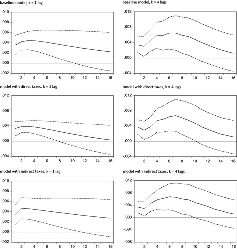
The robustness checks of our analysis were provided by changing the frameworks of the system. At first, the different tax measures were employed through disaggregating the tax data. First, taxes on income and wealth were considered as an approximation of direct taxes. However, the difference between these types of taxes and transfers was negative for most of quarterly observations in our sample, and as a result, the tax variable cannot be transformed into log representation. Consequently, the tax variable (not reduced by social transfers, subsidies and interest payments) was entered into the system. Then the appropriate tax elasticities were recalculated and incorporated within each model. The lag structure for the new models was tested, wherein the maximum number of 4 lags was assumed. The use of the SIC criterion indicated the importance of 1 lag in SVARs for each country (on the contrary, the AIC criterion suggested 4 lags in the model for Poland and that for Hungary, with only 1 lag in the Czech Republic’s model). However, the use of 1 lag in the model with direct taxes for Poland was not satisfactory from the point of view of the quality of residuals (due to autocorrelation). As a result, the decision about the model extension was made up to maximum number of lags (i.e., 4). When the model with 4 lags was built for Poland, then the test was not rejected.² The same procedure was repeated for models with indirect taxes (treated as an approximation of taxes on production and imports). The estimated coefficients of A and B matrices are presented in Table A4 and Table A6 in the Appendix; the impulse response functions are illustrated in Figure A3 and Figure A5 in the Appendix. As investigated, the shapes of obtained impulse response functions are quite similar to those of the baseline models. The error bands indicate the non-significant response of output to spending shock in the Czech Republic. The maximum response of Y to G shock is lagged in the case of each country. The peak multipliers calculated for Hungary in models with direct or indirect taxes are higher than in the baseline model, whereas calculations for the Czech Republic present similar values of multipliers (compare Table 1 in the article and Table A10 in the Appendix). In the case of Poland, the peak multiplier for the baseline model is similar to the peak spending multiplier calculated for the model with indirect taxes; also, the quarter with the peak response is the same in both models (although in the case of Poland, due to presented problems with autocorrelation of the residuals, the model with 1 lag was not calculated for the system with direct taxes).

In order to compare effects of spending innovations in models with 4 lags, the additional analysis was prepared. The results for the Czech Republic, Hungary and Poland are presented in Table A5 and Table A7 and Figure A4 and Figure A6 in the Appendix. Due to problems with the quality of the SVAR model in relation to indirect taxes, the calculations for Hungary were not presented. The peak multipliers (adjusted to be interpreted in the national currency) are reported, as previously, in Table A10.

In the study, models with 4 lags in the baseline representation were also investigated. The impulse response functions for Y variable are illustrated in Figure A7 in the Appendix (Table A8 in the Appendix includes the elements of A and B matrices). As presented, the inclusion of 4 lags provides a more significant reaction of Y to the structural one standard deviation shock in G. The calculated peak multipliers are higher than in the baseline model, even if the same system of variables is analysed (see Table A10 in the Appendix). The obtained outcome is consistent with the conclusions provided in Čapek and Crespo Cuaresma (2018), in that the peak multiplier calculated in the SVAR model with 4 lags is higher than that calculated in a similar model with a lower number of lags. Table 2 below presents the cumulative multipliers estimated for extended models. These models are stable (all unit roots are inside the unit circle). The calculation of multipliers follows the same procedure, as previously.

Table 2. Spending multipliers: baseline model with k = 4 lags.

	Cumulative multiplier after quarter			Peak multiplier
	4th	8th	16th
Czech Republic	0.3409	0.8582	1.4356	0.2430 (6)
Hungary	0.6462	1.0319	1.5827	0.6725 (3)*
Poland	1.2456	1.5969	1.8798	2.2880 (7)*

Notes: In the case of the peak multiplier, the sign * denotes the significance of the calculation based on the error bands. The number in brackets denotes the quarter with the maximum response. The calculation of the cumulative multiplier is based on the accumulated responses, whereas the calculation of the peak multiplier is based on the responses of Y to the initial one standard deviation shock in G.

Source: Author’s own calculations.

Finally, the investigation of whether the response of Y to G shock depends on the period of analysis was conducted. Although the sample under consideration is quite short, the decision to extract the ‘turbulent times’ was made. As a result, the baseline sample was shortened to a sample covering the period since 2007, i.e., the period with serious macroeconomic turbulences (including a crisis period) in many countries; this division is similar to that in Mirdala and Kamenik (2017). The lag length test, based again on the SIC criterion, indicates the inclusion of 1 lag in the case of each country. The implication of 1 lag ensures the stability of each model. Taking into account the model specifications (without the ‘crisis’ dummy variable) and the same values of tax elasticities as those incorporated into the baseline model, the impulse response functions were obtainable only for Hungary and Poland (see Figure A8 and Table A9 in the Appendix). In the case of the Czech Republic, the analysis based on the same assumptions and exogenous elasticities did not allow the estimation of satisfactory parameters of the A and B matrices.³ In these two countries, the maximum response is lagged: in Poland it occurs after the 2nd quarter, whereas in the case of Hungary after the 7th quarter. The value of the peak multipliers is presented in Table A10 of the Appendix. Due to the quite short sample, problems with obtaining satisfactory results for the pre-crisis sample occurred: the analysis based on the same assumptions and exogenous elasticities did not allow the estimation of satisfactory parameters of the A and B matrices⁴ or did not ensure the good quality of the residuals.

The analysis of the calculated multipliers and the observation of impulse response functions (error bands) indicate that the results for Poland were not satisfactory. Subsequently, the models for Poland were re-estimated. The new specification includes, as previously, the same variables and the trend variable, but without the dummy variable for the crisis and post-crisis period. The new elements of A and B matrices are presented in Table A11 in the Appendix, while Figure A9 in the Appendix shows impulse response functions for Poland. As presented in Table 3 below, the SVAR specification without the ‘crisis’ dummy variable leads to lower peak multipliers. However, their values are still higher than 1.

Table 3. Peak spending multipliers for Poland; specifications without the ‘crisis’ dummy variable.

Baseline model, k = 1 lag	Baseline model, k = 4 lags	Model with direct taxes, k = 1 lag	Model with direct taxes, k = 4 lags	Model with indirect taxes, k = 1 lag	Model with indirect taxes, k = 4 lags
1.21 (3)*	1.80 (7)*	1.08 (3)*	2.00 (7)*	1.29 (2)*	2.06 (6)*

Notes: * denotes the significance of the calculation based on the error bands. The number in brackets denotes the quarter with the maximum response.

Source: Author’s own calculations.

The literature review provides results for multipliers in other CEE countries. For instance, Grdović Gnip (2014) received a cumulative spending multiplier for Croatia that was equal to 1.84 after 12 quarters, and 2.66 after 20 quarters. Mirdala (2009) reported a positive response of GDP to government spending shock for the Czech Republic, Hungary, Poland, Romania, Bulgaria and the Slovak Republic. Haug et al. (2013) in their SVAR for Poland (1998q1–2012q4) calculated spending multipliers lower than those in our study: the estimated values range between 0.14 after the first quarter to 0.48 after 12 quarters (peak multiplier). Lendvai’s (2007) work shows a negative response of GDP to expansionary spending shock in Hungary (SVAR estimated for the period 1997q1–2005q4).

However, in the light of the literature, the obtained results are quite similar to calculations of spending multiplier for the eurozone countries. For example, Afonso and Silva Leal (2018) in their baseline SVAR calculate the accumulated spending multiplier (for primary expenditure) as equal to 0.64 after 4 quarters and 1.10 after 8 quarters (the sample covers 2001q1–2016q4, composed of 19 eurozone countries with dummy variables related to their membership). The short-term multiplier in Burriel et al. (2010) study of the eurozone is calculated as 0.87. In Borg’s (2014) study, the cumulative spending multiplier for Malta reaches 1.0 in the 4th quarter and 1.2 in the 8th quarter after shock. Perotti (2005) obtains the cumulative GDP response to spending shock in the 4th quarter as equal to 0.4 in Germany, whereas the spending multipliers calculated by Tenhofen et al. (2010) are: 0.83 on impact, 0.58 after 4 quarters, 0.4 after 8 quarters, and close to zero after 12 quarters (however, these two works do not cover a sample that includes the latest crisis period). The short-term cumulative spending multiplier calculated by de Castro Fernández and Hernández de Cos (2006) for Spain is higher than 1 (the value is 1.31), whereas it decreases to 0.26 after 20 quarters. Finally, as presented by Mineshima, Poplawski-Ribeiro, and Weber (2014), the first-year spending multipliers calculated for European countries with the linear VAR framework range from 0.3 (minimum) to 1.8 (maximum) whereas the median is 0.8.

6. Conclusion

The aim of this article is to compare the effects of government spending shock in three CEE countries: the Czech Republic, Hungary and Poland. The analysis uses SVAR with the identification scheme based on that of Blanchard and Perotti (2002). The results indicate the positive response of output to the government spending shock. The baseline model specification, including the same assumptions for each country, provides peak multipliers (adjusted to be interpreted in the national currency) ranging from 0.2 in the Czech Republic to 1.8 in Poland. Generally, these multipliers for the Czech Republic and Hungary correspond to the findings in the existing literature; however, in the case of Poland the calculated peak value is much higher than 1.

In accordance with the results, it is important to emphasise some issues related to the analysed models. The presented estimations are based on quite a short sample of 65 quarterly observations, moreover the three-variable system is employed. The length of time series can affect the results, in that the calculated multipliers may be biased (this problem is especially related to the multipliers calculated for the ‘turbulent times’). Another comment concerns the elements of matrix A in the AB-representation. As presented, the estimations are based on partial elasticities derived from the exogenous study. Also, the employed tax data are widely aggregated, and based on the ESA2010 approach. Moreover, the calculation of the peak multipliers is based on the mean of GDP to spending ratio over the analysed sample. Finally, as presented by Caldara and Kamps (2012, 2017) for example, the results may be sensitive to the identification scheme, or calculated elasticities. Moreover, the same VAR specification is used in the case of each country. As indicated, with the same model specification, the multipliers for Poland differ from these calculated for the Czech Republic and Hungary, as well as those provided in the literature. The removal of the dummy variable for the crisis and post-crisis period decreased calculated peak multipliers for Poland, however the multipliers are still higher than 1.

The employment of the robustness checks analysis cannot provide any substantial differences between the calculations of the peak multiplier. However, estimated models indicate higher effectiveness of government spending shocks during the period of economic crash. The analysed responsiveness of the output to the spending shock is generally higher during the weak macroeconomic conditions.

The results indicate that in the analysed countries, the effective output stabilisation is made possible by public investment and public consumption. As presented, the calculation of the spending multiplier may to some extent be considered as robust to the change in tax definition. The presented results may contribute to discussions about the effectiveness of government spending stabilisation during these countries’ path to the eurozone. As presented, spending can be used as an effective stabilising tool, as the calculated multipliers are close to 1 or even higher. The spending-based expansionary policy seems to be effective in stimulating economy during the crisis period. Moreover, the effects of spending in the Czech Republic and Hungary are similar to those provided in the literature for the eurozone countries.

Acknowledgements

The author is grateful to the anonymous reviewers for their constructive remarks and useful comments.

Notes

1 In this study the dummy variable is incorporated like in other studies on the subject. However, when the dummy variable is incorporated only for the initial part of the crisis (i.e. in 2008 and 2009), then the value of the calculated multiplier is lower for Poland and higher in the cases of the Czech Republic and Hungary. The results are not reported here.

2 Although with a weaker quality of the residuals than in the cases of the Czech Republic and Hungary.

3 The Hessian matrix was near to singular.

4 Due to the Hessian matrix was near to singular.

Appendix

Table A1. Unit root test for variables (data in log).

		Regression with trend and constant			Regression with constant, without trend
		Czech Republic	Hungary	Poland	Czech Republic	Hungary	Poland
ADF	$G_t$	–2.7206 (0.2316)	–2.8602 (0.1814)	–1.1631 (0.9088)	–2.2371 (0.1952)	–2.8059 (0.0626)	–1.7197 (0.4163)
	$R_t$	–4.7563 (0.0013)	–2.3328 (0.4112)	–2.2715 (0.4429)	–1.5394 (0.5084)	–0.8543 (0.7972)	–1.2623 (0.6420)
	$Y_t$	–1.5684 (0.7962)	–1.8707 (0.6597)	–1.6074 (0.7792)	–1.1731 (0.6821)	–1.3303 (0.6115)	–0.9159 (0.7771)
	${\Delta G}_t$	–13.8233 (0.0001)	–2.2971 (0.4297)	–3.8366 (0.0212)	–13.8347 (0.0001)	–2.2201 (0.2012)	–3.5577 (0.0096)
	${\Delta R}_t$	–14.2564 (0.0001)	–8.5978 (0.0000)	–5.4798 (0.0001)	–14.3539 (0.0001)	–8.6792 (0.0000)	–5.5089 (0.0000)
	${\Delta Y}_t$	–5.6657 (0.0001)	–4.8414 (0.0010)	–9.2605 (0.0000)	–5.6420 (0.0000)	–4.8595 (0.0001)	–9.2144 (0.0000)
PP	$G_t$	–3.6673 (0.0308)	–2.0428 (0.5686)	–1.1479 (0.9122)	–1.3144 (0.6191)	–1.9448 (0.3105)	–1.6419 (0.4556)
	$R_t$	–4.9045 (0.0008)	–6.7690 (0.0000)	–2.1944 (0.4843)	–2.0489 (0.2658)	–2.7898 (0.0645)	–1.2238 (0.6592)
	$Y_t$	–1.6519 (0.7627)	–1.9805 (0.6023)	–1.6015 (0.7816)	–1.3144 (0.6191)	–1.7172 (0.4186)	–0.9455 (0.7673)
	${\Delta G}_t$	–19.9127 (0.0001)	–9.5100 (0.0000)	–8.6616 (0.0000)	–17.0958 (0.0001)	–9.5094 (0.0000)	–8.5109 (0.0000)
	${\Delta R}_t$	–20.1116 (0.0001)	–21.7084 (0.0001)	–9.1319 (0.0000)	–20.4093 (0.0001)	–23.3750 (0.0001)	–9.2023 (0.0000)
	${\Delta Y}_t$	–5.8311 (0.0000)	–4.7965 (0.0011)	–9.1746 (0.0000)	–5.8008 (0.0000)	–4.8052 (0.0002)	–9.1204 (0.0000)

Notes: p-values in brackets, ADF – Augmented Dickey-Fuller test, PP – Phillips–Perron test, $\Delta$ refers to the first differences.

Table A2. Lag length criteria for the baseline model.

		0	1	2	3	4
AIC	Czech Republic	–8.696246	–12.01446*	–11.97899	–11.89634	–11.85934
	Hungary	–9.128542	–12.03836*	–11.94079	–11.73642	–11.82031
	Poland	–12.05529	–15.09811*	–14.99771	–14.90429	–14.83318
SIC	Czech Republic	–8.395177	–11.41232*	–11.07579	–10.69206	–10.35400
	Hungary	–8.827473	–11.43623*	–11.03758	–10.53215	–10.31497
	Poland	–11.74385	–14.47523*	–14.06339	–13.65853	–13.27598
HQC	Czech Republic	–8.577455	–11.77687*	–11.62262	–11.42117	–11.26539
	Hungary	–9.009751	–11.80078*	–11.58442	–11.26126	–11.22636
	Poland	–11.93324	–14.85400*	–14.63154	–14.41606	–14.22290

Notes: * Denotes the lag order selected by the criterion, AIC – Akaike information criterion, SIC – Schwarz information criterion, HQC – Hannan–Quinn information criterion.

Table A3. Elements of A and B matrices for the baseline model.

	$a_4$	$a_5$	$b_1$	$b_2$	$b_4$	$b_3$	$a_6$
Czech Republic	0.018 (0.529)	–0.002 (0.894)	0.058 (0.000)	0.009 (0.000)	0.070 (0.000)	0.061 (0.000)	0.96
Hungary	0.044 (0.040)	0.002 (0.855)	0.042 (0.000)	0.007 (0.000)	–0.016 (0.202)	0.099 (0.000)	0.98
Poland	0.230 (0.000)	–0.012 (0.479)	0.016 (0.000)	0.007 (0.000)	0.013 (0.054)	0.054 (0.000)	1.15

Notes: p-values in brackets; ${\mathrm{a}}_6$ is exogenously-calculated average elasticity.

Table A4. Elements of A and B matrices – model with direct taxes, k = 1 lag.

	$a_4$	$a_5$	$b_1$	$b_2$	$b_4$	$b_3$	$a_6$
Czech Republic	0.021 (0.257)	–0.004 (0.950)	0.059 (0.000)	0.009 (0.000)	0.001 (0.999)	0.019 (0.000)	0.27
Hungary	0.091 (0.009)	–0.031 (0.127)	0.029 (0.000)	0.007 (0.000)	0.019 (0.001)	0.045 (0.000)	0.29
Poland*	×	×	×	×	×	×	0.05

Notes: p-values in brackets; ${\mathrm{a}}_6$ is exogenously-calculated average elasticity.

* In the case of Poland, x denotes a lack of satisfactory models.

Table A5. Elements of A and B matrices – model with direct taxes, k = 4 lags.

	$a_4$	$a_5$	$b_1$	$b_2$	$b_4$	$b_3$	$a_6$
Czech Republic	0.015 (0.359)	–0.007 (0.891)	0.062 (0.000)	0.008 (0.000)	0.001 (0.796)	0.019 (0.000)	0.27
Hungary	0.073 (0.066)	–0.021 (0.298)	0.024 (0.000)	0.007 (0.000)	0.014 (0.018)	0.045 (0.000)	0.29
Poland	0.224 (0.000)	0.072 (0.035)	0.015 (0.000)	0.007 (0.000)	0.003 (0.350)	0.025 (0.000)	0.05

Notes: p-values in brackets; ${\mathrm{a}}_6$ is exogenously-calculated average elasticity.

Table A6. Elements of A and B matrices – model with indirect taxes, k = 1 lag.

	$a_4$	$a_5$	$b_1$	$b_2$	$b_4$	$b_3$	$a_6$
Czech Republic	0.026 (0.125)	0.101 (0.003)	0.059 (0.000)	0.009 (0.000)	–0.003 (0.341)	0.029 (0.000)	0.34
Hungary	0.116 (0.001)	0.044 (0.050)	0.029 (0.000)	0.007 (0.000)	–0.011 (0.037)	0.040 (0.000)	0.45
Poland	0.179 (0.001)	0.025 (0.124)	0.016 (0.000)	0.007 (0.000)	0.013 (0.036)	0.048 (0.000)	0.87

Notes: p-values in brackets; ${\mathrm{a}}_6$ is exogenously-calculated average elasticity.

Table A7. Elements of A and B matrices – model with indirect taxes, k = 4 lags.

	$a_4$	$a_5$	$b_1$	$b_2$	$b_4$	$b_3$	$a_6$
Czech Republic	0.024 (0.130)	0.098 (0.003)	0.062 (0.000)	0.008 (0.000)	–0.004 (0.284)	0.029 (0.000)	0.34
Hungary*	×	×	×	×	×	×	0.45
Poland	0.213 (0.001)	0.016 (0.369)	0.015 (0.000)	0.007 (0.000)	0.016 (0.007)	0.046 (0.000)	0.87

Notes: p-values in brackets; ${\mathrm{a}}_6$ is exogenously-calculated average elasticity.

* In the case of Hungary, × denotes a lack of satisfactory models.

Table A8. Elements of A and B matrices – the baseline model with 4 lags.

	$a_4$	$a_5$	$b_1$	$b_2$	$b_4$	$b_3$	$a_6$
Czech Republic	0.012 (0.664)	0.001 (0.966)	0.063 (0.000)	0.008 (0.000)	0.076 (0.000)	0.055 (0.000)	0.96
Hungary	0.077 (0.025)	–0.005 (0.583)	0.025 (0.000)	0.007 (0.000)	–0.012 (0.316)	0.098 (0.000)	0.98
Poland	0.249 (0.001)	–0.020 (0.249)	0.016 (0.000)	0.007 (0.000)	0.010 (0.159)	0.056 (0.000)	1.15

Notes: p-values in brackets; ${\mathrm{a}}_6$ is exogenously-calculated average elasticity.

Table A9. Elements of A and B matrices – subsample since 2007.

	$a_4$	$a_5$	$b_1$	$b_2$	$b_4$	$b_3$	$a_6$
Czech Republic*	×	×	×	×	×	×	0.96
Hungary	0.166 (0.072)	0.006 (0.802)	0.027 (0.000)	0.009 (0.000)	0.037 (0.000)	0.061 (0.000)	0.98
Poland	0.235 (0.001)	0.016 (0.519)	0.017 (0.000)	0.007 (0.000)	0.005 (0.448)	0.043 (0.000)	1.15

Notes: p-values in brackets; ${\mathrm{a}}_6$ is exogenously-calculated average elasticity.

* In the case of the Czech Republic, × denotes a lack of satisfactory models.

Table A10. Peak multipliers (adjusted to be interpreted in the national currency) in robust system specifications.

	Direct taxes	Indirect taxes	Direct taxes, k = 4 lags	Indirect taxes, k = 4 lags	Baseline model, k = 4 lags	Baseline model, sample since 2007
Czech Republic	0.1753 (3)	0.1719 (3)	0.2453 (6)	0.3429 (6)*	0.2430 (6)	×
Hungary	0.4529 (4)*	0.8514 (7)*	0.4602 (5)	×	0.6725 (3)*	0.6774 (7)
Poland	×	1.8335 (7)*	2.1727 (7)*	2.2655 (7)*	2.2880 (7)*	1.0744 (1)*

Notes: * Denotes significance based on the error bands; the quarter with the peak value is in brackets; × indicates a lack of satisfactory models.

Table A11. Elements of A and B matrices, the additional SVAR specification for Poland.

	$a_4$	$a_5$	$b_1$	$b_2$	$b_4$	$b_3$	$a_6$
baseline model, k = 1 lag	0.206 (0.000)	0.009 (0.555)	0.016 (0.000)	0.007 (0.000)	0.013 (0.088)	0.059 (0.000)	1.15
baseline model, k = 4 lags	0.219 (0.001)	0.001 (0.988)	0.016 (0.000)	0.001 (0.000)	0.011 (0.166)	0.061 (0.000)	1.15
model with direct taxes, k = 1 lag	0.184 (0.001)	0.091 (0.001)	0.016 (0.000)	0.007 (0.000)	0.003 (0.412)	0.034 (0.000)	0.05
model with direct taxes, k = 4 lags	0.221 (0.000)	0.099 (0.001)	0.015 (0.000)	0.006 (0.000)	0.003 (0.337)	0.029 (0.000)	0.05
model with indirect taxes, k = 1 lag	0.166 (0.002)	0.042 (0.008)	0.016 (0.000)	0.007 (0.000)	0.013 (0.045)	0.051 (0.000)	0.87
model with indirect taxes, k = 4 lags	0.194 (0.002)	0.029 (0.096)	0.015 (0.000)	0.007 (0.000)	0.015 (0.010)	0.047 (0.000)	0.87

Notes: p-values in brackets; ${\mathrm{a}}_6$ is exogenously-calculated average elasticity.

Figure A1. Inverse roots of AR Characteristic Polynomial for baseline model.

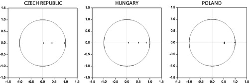
Figure A2. Impulse responses of Y to structural one s.d. shock in G ± 2 s.e., baseline model.

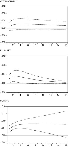
Figure A3. Impulse responses of Y to structural one s.d. shock in G ± 2 s.e., model with direct taxes, k = 1 lag.

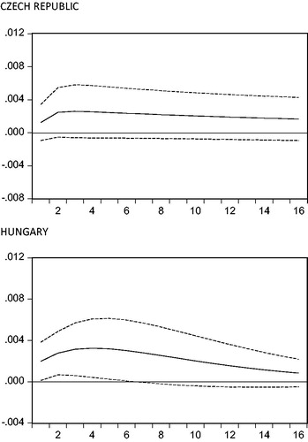
Figure A4. Impulse responses of Y to structural one s.d. shock in G ± 2 s.e., model with direct taxes, k = 4 lags.

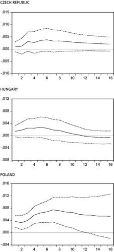
Figure A5. Impulse responses of Y to structural one s.d. shock in G ± 2 s.e., model with indirect taxes, k = 1 lag.

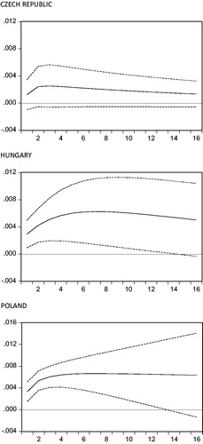
Figure A6. Impulse responses of Y to structural one s.d. shock in G ± 2 s.e., model with indirect taxes, k = 4 lags.

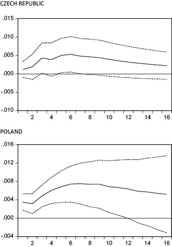
Figure A7. Impulse responses of Y to structural one s.d. shock in G ± 2 s.e., baseline SVAR with k = 4 lags.

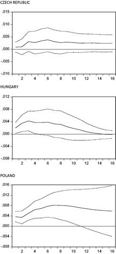
Figure A8. Impulse responses of Y to structural one s.d. shock in G ± 2 s.e., subsample since 2007.

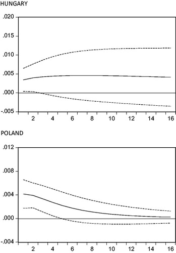
Figure A9. Impulse responses of Y to structural one s.d. shock in G ± 2 s.e. for Poland, SVAR specifications without the dummy variable for the crisis and post-crisis period.

References

- Afonso, A., & Silva Leal, F. (2018). Fiscal multipliers in the Eurozone: A SVAR analysis. Working Papers REM 2018/47, ISEG - Lisbon School of Economics and Management.
- Afonso, A., Baxa, J., & Slavik, M. (2018). Fiscal developments and financial stress: A threshold VAR analysis. Empirical Economics, 54(2), 395–423. doi:10.1007/s00181-016-1210-5
- Auerbach, A. J., & Gorodnichenko, Y. (2012). Measuring the output responses to fiscal policy. American Economic Journal: Economic Policy, 4(2), 1–27. doi:10.1257/pol.4.2.1
- Baranowski, P., Krajewski, P., Mackiewicz, M., & Szymańska, A. (2016). The effectiveness of fiscal policy over the business cycle: A CEE perspective. Emerging Markets Finance and Trade, 52(8), 1910–1921. doi:10.1080/1540496X.2015.1046335
- Batini, N., Callegari, G., & Melina, G. (2012). Successful austerity in the United States, Europe and Japan. IMF Working Papers WP12/190doi:10.5089/9781475505382.001
- Batini, N., Eyraud, L., & Weber, A. (2014). A simple method to compute fiscal multipliers. IMF Working Papers no. WP/14/93doi:10.5089/9781498357999.001
- Baum, A., & Koester, G. B. (2011). The impact of fiscal policy on economic activity over the business cycle – Evidence from a threshold VAR analysis. Bundesbank Discussion Paper No. 3, Series 1, Deutsche Bundesbank.
- Benčík, M. (2014). Dual regime fiscal multipliers in converging economies – A simple STVAR approach. Národná Banka Slovenska, Working Paper no. 2/2014.
- Biau, O., & Girard, E. (2005). Politique budgétaire et dynamique économique en France: L’approche VAR structurel. Economie Prevision, (3), 1–23.
- Blanchard, O., & Perotti, R. (2002). An empirical characterization of the dynamic effects of changes in government spending and taxes on output. The Quarterly Journal of Economics, 117(4), 1329–1368. doi:10.1162/003355302320935043
- Borg, I. (2014). Fiscal multipliers in Malta. Central Bank of Malta Working Paper no. WP/06/2014.
- Burriel, P., De Castro, F., Garrote, D., Gordo, F., Paredes, J., & Pérez, J. (2010). Fiscal policy shocks in the Euro Area and the US: An empirical assessment. Fiscal Studies, 31(2), 251–285. doi:10.1111/j.1475-5890.2010.00114.x
- Caldara, D., & Kamps, C. (2008). What are the effects of fiscal policy shocks? A VAR-based comparative analysis. ECB Working Papers series no 877.
- Caldara, D., & Kamps, C. (2012). The analytics of SVARs: A unified framework to measure fiscal multipliers. Washington, DC: Finance and Economics Discussion Series Divisions of Research & Statistics and Monetary Affairs Federal Reserve Board.
- Caldara, D., & Kamps, C. (2017). The analytics of SVARs: A unified framework to measure fiscal multipliers. The Review of Economic Studies, 84(3), 1015–1040. doi:10.1093/restud/rdx030
- Canova, F. (2007). Methods for applied macroeconomic research. Princeton, NJ: Princeton University Press.
- Čapek, J., & Crespo Cuaresma, J. (2018). We just estimated twenty million fiscal multipliers. Vienna University of Economics and Business, Department of Economics Working Paper no. 268
- Christiano, L. J., Eichenbaum, M., & Rebelo, S. (2011). When is the government spending multiplier large? Journal of Political Economy, 119(1), 78–121. doi:10.1086/659312
- Coenen, G., Erceg, C. J., Freedman, C., Furceri, D., Kumhof, M., Lalonde, R., … in’t Veld, J. (2012). Effects of fiscal stimulus in structural models. American Economic Journal: Macroeconomics, 4(1), 22–68. doi:10.1257/mac.4.1.22
- Cogan, J. F., Cwik, T., Taylor, J. B., & Wieland, V. (2010). New Keynesian versus Old Keynesian government spending multipliers. Journal of Economic Dynamics and Control, 34 (3), 281–295. doi:10.1016/j.jedc.2010.01.010
- Ćorić, T., Šimović, H., & Deskar-Škrbić, M. (2015). Monetary and fiscal policy mix in a small open economy: The case of Croatia. Economic Research-Ekonomska Istraživanja, 28(1), 407–421. doi:10.1080/1331677X.2015.1059073
- Crespo Cuaresma, J., Eller, M., & Mehrotra, A. (2011). The economic transmission of fiscal policy shocks from Western to Eastern Europe. BOFIT Discussion Papers, 12.
- de Castro Fernández, F., & Hernández de Cos, P. (2006). The economic effects of exogenous fiscal shocks in Spain. A SVAR approach. EBC Working Paper Series No 647.
- Deskar-Škrbić, M., Drezgić, S., & Šimović, H. (2018). Tax policy and labour market in Croatia: Effects of tax wedge on employment. Economic Research-Ekonomska Istraživanja, 31(1), 1218–1227. doi:10.1080/1331677X.2018.1456359
- Deskar-Škribić, M., & Šimović, H. (2017). The effectiveness of fiscal spending in Croatia, Slovenia and Serbia: The role of trade openness and public debt level. Post-Communist Economies, 29(3), 336–358. doi:10.1080/14631377.2016.1267972
- Eggertsson, G. (2011). What fiscal policy is effective at zero interest rates? NBER Macroeconomics Annual, 25(1), 59–112. doi:10.1086/657529
- Erceg, C., & Lindé, J. (2014). Is there a fiscal free lunch in a liquidity trap? Journal of the European Economic Association, 12(1), 73–107. doi:10.1111/jeea.12059
- Fatás, A., & Mihov, I. (2001). The effects of fiscal policy on consumption and employment: Theory and evidence, CEPR Discussion Papers, 2760.
- Favero, C., & Giavazzi, F. (2012). Measuring tax multipliers: The narrative method in fiscal VARs. American Economic Journal: Economic Policy, 4(2), 69–94. doi:10.1257/pol.4.2.69
- Forni, M., & Gambetti, L. (2016). Government spending shocks in open economy VARs. Journal of International Economics, 99, 68–84. doi:10.1016/j.jinteco.2015.11.010
- Gechert, S., & Rannenberg, A. (2014). Are fiscal multipliers regime-dependent? A meta-regression analysis. IMK Working Paper No, 139.
- Gechert, S. (2015). What fiscal policy is most effective? A meta-regression analysis. Oxford Economic Papers, 67(3), 553–580. doi:10.1093/oep/gpv027
- Giordano, R., Momigliano, S., Neri, S., & Perotti, R. (2007). The effects of fiscal policy in Italy: Evidence from a VAR model. European Journal of Political Economy, 23(3), 707–733. doi:10.1016/j.ejpoleco.2006.10.005
- Grdović Gnip, A. (2014). The power of fiscal multipliers in Croatia. Financial Theory and Practice, 38(2), 173–219.
- Hall, R. E. (2009). By how much does GDP rise if the government buys more output? Brookings Papers on Economic Activity, 2009(Fall), 183–231.
- Haug, A., Jędrzejowicz, T., & Sznajderska, A. (2013). Combining monetary and fiscal policy in an SVAR for a small open economy. NBP Working Paper no. 168.
- Hemming, R., Kell, M., & Mahfouz, S. (2002). The effectiveness of fiscal policy in stimulating economic activity-a review of the literature. IMF Working Paper No. 02/208.
- Hinić, B., & Miletić, M. (2013). Efficiency of the fiscal and monetary stimuli: The case of Serbia (mimeo), National Bank of the Republic of Macedonia, Skopje. http://www.nbrm.mk/WBStorage/Files/WebBuilder_Mirjana_Miletic_Presentation_2ndNBRMConference.pdf.
- Ilzetzki, E., Mendoza, E. G., & Végh, C. A. (2013). How big (small?) Are fiscal multipliers? Journal of Monetary Economics, 60(2), 239–254. doi:10.1016/j.jmoneco.2012.10.011
- IMF. (2017). Structural Fiscal Balances. www.imf.org.
- Kraay, A. (2014). Government spending multipliers in developing countries: Evidence from lending by official creditors. American Economic Journal: Macroeconomics, 6(4), 170–208. doi:10.1257/mac.6.4.170
- Lendvai, J. (2007). The impact of fiscal policy in Hungary. ECFIN Country Focus, 4(11), 1–6.
- Lütkepohl, H. (2005). New introduction to multiple time series analysis. New York: Springer.
- Mertens, K., & Ravn, M. O. (2012). Empirical evidence on the aggregate effects of anticipated and unanticipated US tax policy shocks. American Economic Journal: Economic Policy, 4(2), 145–181. doi:10.1257/pol.4.2.145
- Mertens, K., & Ravn, M. O. (2014). A reconciliation of SVAR and narrative estimates of tax multipliers. Journal of Monetary Economics, 68, S1–S19. doi:10.1016/j.jmoneco.2013.04.004
- Mineshima, A., Poplawski-Ribeiro, M., & Weber, A. (2014). Size of fiscal multipliers. In Cottarelli, C., Gerson, P., Senhadji, A., & Semlali, A. S. (Eds.), Post-crisis fiscal policy, pp. 315–372. Cambridge, MA: MIT Press.
- Mirdala, R. (2009). Effects of fiscal policy shocks in the European transition economies. Journal of Applied Research in Finance, 1(2), 141–155.
- Mirdala, R., & Kamenik, M. (2017). Effects of fiscal policy shocks in CE3 countries (TVAR approach). E + M Ekonomie a Management, 2, 46–64. doi:10.15240/tul/001/2017-2-004
- Monacelli, T., & Perotti, R. (2008). Fiscal policy, wealth effects, and markups. NBER Working Papers no. 14584, National Bureau of Economic Research, Inc.
- Mountford, A., & Uhlig, H. (2009). What are the effects of fiscal policy shocks? Journal of Applied Econometrics, 24(6), 960–992. doi:10.1002/jae.1079
- Owyang, M. T., Ramey, V. A., & Zubairy, S. (2013). Are government spending multipliers greater during periods of slack? Evidence from twentieth-century historical data. American Economic Review, 103(3), 129–134. doi:10.1257/aer.103.3.129
- Perotti, R. (2005). Estimating the effects of fiscal policy in OECD countries. CEPR Discussion Paper No. 4842.
- Ramey, V. A. (2011). Identifying government spending shocks: It’s all in the timing. The Quarterly Journal of Economics, 126(1), 1–50. doi:10.1093/qje/qjq008
- Ramey, V. A., & Shapiro, M. D. (1998). Costly capital reallocation and the effects of government spending. Carnegie-Rochester Conference Series on Public Policy, 48(1), 145–194. doi:10.1016/S0167-2231(98)00020-7
- Ramey, V. A., & Zubairy, S. (2018). Government spending multipliers in good times and in bad: Evidence from US historical data. Journal of Political Economy, 126(2), 850–901. doi:10.1086/696277
- Ravnik, R., & Žilić, I. (2011). The use of SVAR analysis in determining the effects of fiscal shocks in Croatia. Financial Theory and Practice, 35, 25–58.
- Romer, C. D., & Romer, D. H. (2010). The macroeconomic effects of tax changes: Estimates based on a new measure of fiscal shocks. American Economic Review, 100(3), 763–801. doi:10.1257/aer.100.3.763
- Sekuła, A., & Śmiechowicz, J. (2016). Systems of general grants for local governments in selected EU countries against the background of the general theory of fiscal policy. Equilibrium, 11(4), 711–734. doi:10.12775/EQUIL.2016.032
- Szörfi, B., & Tóth, M. (2018). Measures of slack in the euro area. In ECB Economic Bulletin, Issue 3, Box 3, 31–35.
- Šimović, H. (2017). Impact of public debt (un)sustainability on fiscal policy effectiveness in Croatia. EFZG Working Paper Series no. 17-05.
- Šimović, H., & Deskar-Škrbić, M. (2013). Dynamic effects of fiscal policy and fiscal multipliers in Croatia. Zbornik Radova Ekonomskog Fakulteta u Rijeci: časopis za Ekonomsku Teoriju i Praksu, 31(1), 55–78.
- Sims, C. (1980). Macroeconomics and reality. Econometrica, 48(1), 1–49. doi:10.2307/1912017
- Sims, C., Stock, J., & Watson, M. W. (1990). Inference in linear time series models with some unit roots. Econometrica, 58(1), 113–144. doi:10.2307/2938337
- Spilimbergo, A., Symansky, S., & Schindler, M. (2009). Fiscal multipliers, IMF Staff Position Note, no. SPN/09/11. doi:10.5089/9781462372737.004
- Tenhofen, J., Wolff, G. B., & Heppke-Falk, K. H. (2010). The macroeconomic effects of exogenous fiscal policy shocks in Germany: A disaggregated SVAR analysis. Jahrbücher für Nationalökonomie und Statistik, 230(3), 328–355.
- Uhlig, H. (2005). What are the effects of monetary policy on output? Results from an agnostic identification procedure. Journal of Monetary Economics, 52(2), 381–419.