Zero-coupon interest rates: Evaluating three alternative datasets

Abstract

The zero-coupon yield curve is a common input for most financial purposes. We consider three popular yield curve datasets and explore the extent to which the decision as to what dataset to use for a particular application may have an impact on the results. Many term structure papers evaluate alternative models for estimating zero coupon bonds based on their ability to replicate bond prices. However, in this paper we take a step forward by analyzing the consequences of using these alternative datasets in estimates of other moments and variables such as interest rate volatilities or the resulting forward rates and their correlations. After finding significant differences, we also explore the existence of volatility spillover effects among these three datasets. Finally, we illustrate the relevance of the choice of one particular dataset by examining the differences that may arise when testing the expectations hypothesis. In the conclusions, we provide guidance to end users in selecting a particular dataset.

Keywords:

• Term Structure
• Yield Curve
• Data
• Volatility
• Forward rates
• Correlation Expectations
• Hypothesis

JEL Classification:

• E43
• F31
• G12
• G13
• G15

1. Introduction

The zero-coupon yield curve is a key input for many financial and economic purposes. The risk free interest rates for different maturities determine the current value of future nominal payments. They provide the benchmark for pricing all fixed income securities and their derivatives. Since the valuation of these securities must fit an empirically observable term structure of interest rates, this input is essential for the valuation process. The term structure is also used in the calibration of fixed income valuation models, Greek calculations, risk measurement, and design of hedging strategies. The shape of the zero-coupon yield curve is relevant to theories of macroeconomics, particularly in the area of monetary economics.

Nevertheless, the term structure of zero-coupon interest rates is not directly observable and can only be estimated. There are different approaches to estimating a yield curve, but they are just curve fitting techniques. The literature examines different models and the numerical techniques (e.g., Bliss, 1996; Bolder & Gusba, 2002; Jordan & Mansi, 2003; Bolder, Johnson, & Metzler, 2004; Yallup, 2012; Andreasen, Christensen, & Rudebusch, 2017). These papers focus on the ability of alternative models and methodologies to replicate sets of bond prices. There is no consensus on which method is best. In addition, they require cross-sectional prices from the Treasury bond market and both the proper preparation of the data and the estimation of the yield curve itself can sometimes be burdensome.

Practitioners and researchers usually download the zero-coupon yield curves from a database provider instead of proceeding to estimate them directly from market data. A few yield curve datasets have become popular. Some of them because they are publicly available without charge, other ones because they are offered by the primary financial data providers. In fact, although these alternative yield curve datasets can be assumed as equivalent, they are estimated from different market prices or yields to maturity of different sets of Treasury securities and using different estimation methods. Some final users can select the yield curve dataset solely for the convenience. However, any researcher with some experience working with Treasury yields data should be aware of the interest rates implied by these different datasets are different. But, are all the final users really aware of the real implications of these differences on the results of their applications?

This paper attempts to highlight the potential consequences of the “known” differences among three alternative popular databases, sometimes assumed as equivalent, when one of them is used as input for certain application. To do so, we use a different approach. Instead of considering the ability of risk-free zero-coupon rates to replicate bond prices or yields, we focus on the potential impact of the time series of zero-coupon rate estimates on variables such as interest rate volatilities or correlations between forward rates with different maturities. In addition, we explore potential implications when conducting tests of expectation hypothesis in the spirit of Campbell and Shiller (1991).

We examine three popular zero-coupon yield curves provided by the US Department of Treasury or H.15 (DoT), the Federal Reserve Board (FRB), and Bloomberg (F082). The providers of these three datasets use different techniques – a quasi-cubic hermite spline function (DoT), a weighted Svensson (1994) model (FRB), and a piecewise linear function (F082)–, different cross-sectional market data –market yields (DoT), market prices (FRB), and generic prices (F082)–, and different baskets of assets –on-the-run bills and bonds (DoT), second and further off-the-run bonds (FRB), and all the outstanding (even callable) bonds (F082)–.

Our analysis examines the properties of the raw yield curves, attempting to highlight the effects of the data choice on the level, shape or temporal dynamics of the yield curves. These yield curves are the key input for several proposals, such as the pricing of financial assets or the explanation of the behavior of variables such as expected excess holding period returns, risk premia, inflation or consumption growth (see, e.g., Backus, Gregory, & Zin, 1989; Ang & Piazzesi, 2003; Hördahl, Tristani, & Vestin, 2008). As is well known, macroeconomic factors and yield curve factors interact strongly. The short-end of the yield curve would covariate with the monetary policy instruments under the control of the central bank (see, e.g. Taylor, 1993). The average level of the yield curve is usually associated with the rate of inflation and the slope with the business cycle (see, e.g., Diebold, Rudebusch, & Aruoba, 2006). Macroeconomic factors can be extracted simultaneously from a dynamic factor model for a zero-coupon yield curve using the dynamic Nelson and Siegel (1987) yield curve framework (see, e.g., Diebold & Li, 2006).

A preliminary empirical analysis uses intraday trading data from US Treasury securities to show their yields to maturity and to draw yield curves that are extracted from the three zero-coupon interest rate databases to be compared. We selected two dates in which the adjustment of a yield curve is of special complication. A date with a structure of yields to maturity with two humps (July 5, 2006) and another date with severe liquidity problems (September 9, 1999). We observe mispricing problems of each curve for a specific maturity tranche, i.e. FRB in the very short term and DoT between 2 and 7 years, convexity problems in the long end in the case of FRB, and overfitting problems with sawtooth patterns in the case of DoT and F082.

Since all three databases are estimated from different assets, we cannot analyze the ability of these estimates to replicate prices observed in the market. Instead, we measure the differences among the three yield curves by analyzing the following variables: (1) the volatility term structure, which is the volatility of zero-coupon rates with different maturities; and (2) the correlations among forward interest rates. On the one hand, the term structure of volatilities is a necessary input for calibrating many interest rate models and particularly the so called “volatility consistent models”. Within this category we can find models such as Black, Derman, and Toy (1990) model, one of the most popular tools among practitioners, or some extended versions of Hull and White (1994) model. The current term structure of interest rates is exogenously given in these models. Many financial problems such as product valuations, risk measurements, and hedging strategies, depend on spot interest rate volatilities and correlations. For instance, Value-at-Risk depends, above all, on the volatility of spot interest rates and their correlations.

On the other hand, the forward rate correlations determine dynamic models of term structure (see, e.g. Cox, Ingersoll, & Ross, 1985; Ho & Lee, 1986; Black et al., 1990; Heath, Jarrow, & Morton, 1992, and the LIBOR market model). They are the key input for pricing financial products, such as interest rate caps, floors and swaptions. They are also particularly relevant to macroeconomic issues, such as the ability of forward rates to capture market expectations about future short-term interest rates.

Interest rate volatility is a key variable in multiple analyses beyond the financial economics. These time series of volatility are widely used in the literature to examine, for instance, the effects of monetary policy target movements (see, e.g., Cochrane & Piazzesi, 2002; Piazzesi, 2005), its role as a predictor of the economic cycle (see, e.g., Harvey, 1993; Sill, 1996), the volatility interdependence across markets (see, e.g., Engle, Ito, & Lin, 1990; Fleming & Lopez, 1999; Diebold & Yilmaz, 2012), the asymmetric transmission of volatility related to good news and bad news (see, e.g., Engle, Gallo, & Velucchi, 2012), spillovers and contagion (see, e.g., Baig & Goldfajn, 1999; Forbes & Rigobon, 2001), etc.

The first step of our empirical analysis is focused in the study of the temporal dynamics of the volatilities estimated from the standard deviation for 60-day rolling windows and from a conditional model. We use daily yield curve estimates for the three datasets, i.e. DoT, FRB and F082, in the period 1994–2017. The descriptive statistics of the VTS estimates point to important differences for terms of one year or less, F082 being the most volatile. Using various tests to contrast the significant differences between non-overlapping observations from the VTS time series in terms of mean, median and variance, we obtain how the behavior of the F082 series is different from that of the other two series. The statistically significant differences between DoT and FRB are concentrated in the short end of the curve, although they also appear in intermediate maturities. The results are similar regardless of the method used to estimate volatility. Finally, an analysis of cross-data volatility spillovers shows that the more flexible fitting of F082 can anticipate movements in the other two series.

In a second step, we analyze correlations between forward rates. We also apply a preliminary descriptive analysis and different equality tests of averages, medians and variances between the pairwise correlations series. The best behavior from a theoretical point of view of long-term forwards is observed in the DoT series. In addition, the correlations from the FRB and F082 series are much more unstable.

Our latest analysis focuses on replicating a simple classical test of the expectations hypothesis, specifically the analysis presented by Campbell (1995). We observe that depending on the sample of interest rates used, the result of this test would have been different. The DoT dataset shows the most disparate results with those obtained with the other two datasets, especially in the shortest maturity.

Our analysis shows that there is not an optimal yield curve dataset. Anyway, we provide some guidance as to which criteria should be used to choose among alternative datasets. Final users of the yield curve belong to different worlds, namely the academia and the industry, and so they address different issues and have different goals. The DoT dataset provides on-the-run yield curves with rigid shapes that could be especially appropriate for pricing liquid short-term securities, for calibrating interest rate models, and for other purposes in macroeconomic research, monetary policy, or analysis of investors’ risk preferences. The FRB dataset is the only one that allows obtaining a continuous yield curve without interpolation. These flexible off-the-run yield curves generate low volatility levels for most maturities, which could be suitable for pricing medium- and long-term bonds and for market risk management purposes. Finally, the F082 yield curves provide an accurate view of the current full market situation.

2. Alternative yield curve datasets

2.1. Description

In this paper, we use daily data on three of the most popular risk-free interest rate datasets from January 1994 through December 2017. These datasets contain daily estimations of the term structure of zero-coupon interest rates corresponding to the US Treasury market. Two of those datasets are publicly available from the Federal Reserve Board’s website. As a private alternative, we also consider a dataset only available through a financial data vendor. This is the case of the Bloomberg zero-coupon yield curve from government securities (code F082).

The US Department of Treasury daily fits yield curves from observations of either the yield on the most recently auctioned on-the-run Treasuries, or the yields on the interpolated constant-maturity series (see, Jordan & Mansi, 2003). These yield curves are simultaneously published by the Federal Reserve Board’s website as the “Treasury Constant Maturities” dataset which is included in the “H.15 Selected Interest Rates” data release,¹ and by the US Department of the Treasury’s website (“Daily Treasury Yield Curve Rates”).² As such, we refer this dataset as Department of Treasury (DoT). More difficult to find but even more frequently used, the Federal Reserve Board’s website also offers another daily zero-coupon yield curve included in the “Finance and Economics Discussion Series” section.³ It is linked to the Gürkaynak, Sack, and Wright (2007)’s working paper. For convenience, we refer to this latter set of interest rates as “the FRB dataset”; however, the website indicates as follows: “Note: This is not an official Federal Reserve statistical release.”

Table 1 summarizes some of the main characteristics of these three datasets. The fitting technique is completely different. Each method provides yield curves with different degrees of flexibility (see, e.g., Bliss, 1996; Bolder & Gusba, 2002; Bolder et al., 2004; Yallup, 2012). Some techniques are better to describe the hump that is so frequently observed in yield curves or the behavior of long-term interest rates. Other techniques are more rigid in the adjustment of the current yield curve, but they produce more stable time series of spot rates.

Table 1. Primary characteristics of the considered yield curve datasets.

	U.S. Department of the Treasury (DoT) (Constant Maturity Treasuries, H.15)	Gürkaynak et al. (2007) in Federal Reserve Board (FRB)	Bloomberg (F082)
Fitting technique	Quasi-cubic hermite spline function	Weighted Svensson (1994)	Piecewise linear function
Market data	Close of business bid yields-to-maturity	End-of-day prices	Bloomberg generic prices (quotes over a time window), supplemental proprietary contributor prices or both
Bills	Yes (only 4-, 13-, 26-, 52-weeks)	No	No
On-the-run bonds and notes	Yes (only 2-, 3-, 5-, 7-, 10-, 20-, 30-years)	No	Yes
Remaining straight bonds and notes	No	Yes (excluding the first off-the-run)	Yes, including non-straight bonds (callable…)
Shortest considered maturity	1-month	3-month	Not reported
Reported information	11 maturities (1 m, 3 m, 6 m, 1 y, 2 y, 3 y, 5 y, 7 y, 10 y, 20 y, 30 y)	30 yearly maturities +  Svensson parameters	15 maturities (3 m, 6 m, 1 y to 10 y, 15 y, 20 y, 30 y)
Negative interest rates	No	Yes	Yes

First, the FRB dataset is adjusted applying a weighted version of the well-known and widely used parametric and parsimonious procedure proposed by Svensson (1994). This method is an extension of the Nelson and Siegel (1987) method.⁴ It extends the flexibility and the range of shapes generally seen in yield curves: monotonic forms, humps at various areas of the curve, and s-shapes. As usual, they make the variance of the error term proportional to the modified duration of each security to penalize the valuation errors of the short-term securities. In this manner, a better adjustment on the short-end of the yield curve is enforced. Second, the DoT dataset uses a quasi-cubic Hermite spline function that passes exactly through the yields of a given set of securities with constant maturities (see, Jordan & Mansi, 2000). The theoretical security for each maturity is calculated from composites of quotations obtained by the Federal Reserve Bank of New York. Therefore, DoT does not estimate zero-coupon yield term structures but instead uses simple yield curves relating yields to maturity and terms to maturity. Third, the F082 dataset uses a piecewise linear function, although no more details about the concrete function are reported by Bloomberg.⁵

The second source of discrepancies is the cross-sectional market data used as input for the estimations. The FRB uses end-of-the-day prices but does not identify the specific prices employed. There is no information indicating whether the prices are quoted prices (mid bid-ask, bid or ask prices) or trading prices (last trading price, average daily prices or other prices). The DoT is based on the closing market bid-side yields on actively traded Treasury securities in the over-the-counter market. The quotes for these securities are obtained at or near the 3:30 PM close each trading day. The F082 dataset uses the “Bloomberg generic prices”, supplemental proprietary contributor prices or both.⁶

The third and probably main source of divergences among datasets is the basket of assets included in the estimations of each daily yield curve. The FRB excludes from the estimation all Treasury bills and the on-the-run and “first-off-the run” issues of bonds and notes, bonds with less than three months to maturity, bonds with embedded options, twenty-year bonds since 1996 and “other issues that [they] judgmentally exclude on an ad hoc basis.” Most daily estimates incorporate more than one hundred observations. Conversely, the DoT considers only on-the-run securities, including four maturities of the most recent auction bills (4-, 13-, 26- and 52-week), six maturities of just-issued bonds and notes (2-,3-, 5-. 7-, 10- and 30-year) and a composite rate in the 20-year maturity range. Note that as they consider on-the-run bills and bonds, the resulting yield curve can be interpreted as a par yield curve because these just-issued assets are traded near par. However, coupon bias and forward rate bias may appear and with them, differences between zero-coupon interest rates and par yields, especially for long maturities.⁷ It should be noted that daily yield curve estimations are obtained from eleven daily observations. Finally, the third dataset (F082) considers all outstanding Treasury bonds. In this case, the number of daily observations is larger than two hundred.

The three datasets provide interest rates for several discrete maturities. The maturities range from 1-month (DoT), 3-month (F082), or 1-year (FRB) to 30-year (all the datasets). A relevant aspect is that the FRB dataset includes interesting information for a number of purposes, such as pricing, hedging, etc. It includes the six Svensson model’s parameters resulting from each daily estimation, which allows to immediately compute the zero-coupon interest rate for any required maturity. To obtain no reported maturities from the other two datasets requires to use an interpolation method. This interpolation adds additional noise to the estimated interest rates being doubly interpolated.

Recent episodes of extraordinary low levels of interest rates have resulted in negative yields for some Treasury securities on the secondary market.⁸ The DoT considers these negative yields unrelated to the time value of money, consequently the negative input yields are reset to zero percent prior to use as inputs in the yield curve derivation. By contrast, we observe some negative interest rates for the shortest maturities in the case of both the FRB and the F082 datasets.

Table 2 summarizes the descriptive statistics for the time series of continuously compounded spot rates we obtain for the three datasets. In the case of the DoT dataset, we recalculate the reported yield as a continuously compounded interest rate. According to the information on the DoT website, the market yields are investment yields or bond equivalent yields. The formula uses simple interest and the day count convention actual/actual. In addition, the 1-month interest rate is not reported in the F082 dataset. This is also the case of the DoT dataset from the beginning of our sample period (January 1996) up to July 2001. For both cases, we estimate the corresponding interest rate by using cubic interpolation. The table shows a prevalent positive slope of the yield curve. The average spot rate increases as time to maturity grows, from 2.22% for the 1-month rate, to 4.63% for a 30-year maturity. The volatility of the time series increases from approximately 2.13% for monthly rates to 2.22% for 6-month rates, and then goes down to 1.24% for 30-year spot rate.

Table 2. Descriptive statistics of the Term Structure of Interest Rates.

t	Mean			Std. Dev.
	DoT	FRB	F082	DoT	FRB	F082
1-month	2.10	2.45	2.12	2.05	2.20	2.13
3-month	2.19	2.45	2.28	2.12	2.23	2.20
6-month	2.31	2.47	2.42	2.14	2.25	2.26
1-year	2.42	2.56	2.54	2.11	2.25	2.26
2-year	2.68	2.78	2.77	2.06	2.17	2.16
3-year	2.89	3.01	3.01	1.96	2.06	2.05
5-year	3.29	3.45	3.43	1.74	1.85	1.83
7-year	3.62	3.82	3.80	1.60	1.70	1.69
10-year	3.88	4.25	4.10	1.43	1.57	1.49
20-year	4.41	4.83	4.86	1.36	1.42	1.46
30-year	4.37	4.80	4.71	1.28	1.27	1.17
	Min.			Max.
t	DoT	FRB	F082	DoT	FRB	F082
1-month	0.00	−0.11	−1.16	6.09	6.79	6.40
3-month	0.00	−0.02	0.00	6.22	6.68	6.49
6-month	0.02	0.06	0.01	6.34	6.78	6.84
1-year	0.08	0.08	0.04	6.24	7.06	7.07
2-year	0.16	0.16	0.21	6.70	7.08	7.10
3-year	0.28	0.30	0.27	6.65	7.01	7.02
5-year	0.56	0.59	0.61	6.63	7.01	7.01
7-year	0.91	0.95	0.91	6.76	7.14	7.16
10-year	1.36	1.41	1.41	6.82	7.35	7.29
20-year	1.68	1.87	1.85	7.09	7.67	8.05
30-year	2.09	2.38	2.33	6.94	7.67	7.26

This table reports the main descriptive statistics of the zero-coupon interest rates (spot rates) expressed in percentage with continuous compounding from the three daily yield curve datasets (Department of the Treasury, DoT; Federal Reserve Board, FRB; Bloomberg, F082) during the period from January 1996 to December 2017 (5,497 trading days).

Comparing among datasets, we highlight the difference in average levels. As we comment in the next section, DoT and FRB consider completely different Treasury securities according their liquidity. The DoT dataset only considers the most liquid assets, the on-the-run ones, meanwhile the FRB dataset excludes all the bills and the on-the-run and first-off-the-run bonds. The F082 dataset includes all the Treasury securities. As expected, the yearly average spot rates for the DoT are lower than the corresponding rates for the FRB for all the maturity spectrum.

2.2. Implications of the basket of assets

From the previous section, we can highlight that the inputs included to fit the underlying yield curves provided by the three considered risk-free interest rate datasets are plainly different in characteristics and in number of included securities. For instance, they range from eleven to more than two hundred securities. In this section, we comment some of the potential implications of these disparities. The three datasets use exclusively US Treasury securities as input, but these assets have some important features with significant effects on yields. The main differentiating characteristic is the liquidity. Other relevant features to consider are a potential market segmentation, the number and maturity spectrum of the considered securities, and the optionality.

Liquidity is a key factor in the pricing of fixed income securities. Since the seminal work by Amihud and Mendelson (1991), there has been a large literature on how security’s liquidity is priced in Treasury markets. The observed differences in prices imply that market participants price liquidity. Investors are willing to pay a higher price for liquid assets. Otherwise, the more highly liquid securities are traded with a liquidity premium that implies a higher price and therefore a lower yield-to-maturity. Sarig and Warga (1989) show that the “on-the-run” or “just-issued” security is by far the most highly liquid bond and is traded with a liquidity premium on prices. Krishnamurthy (2002), Goldreich, Hanke, and Nath (2005), Díaz and Escribano (2017) examine the “on-the-run/off-the-run” spread and the regular and well-defined trading activity cycle throughout the lifetime of the US Treasury bonds.

In this sense, the criterium employed by both the DoT and the FRB datasets about the considered Treasury assets in their estimation are completely opposite. The DoT only includes on-the-run assets, meanwhile the FRB excludes on-the-run and first-off-the-run assets. The on-the-run bond generally has higher prices than previous issues (off-the-run) that mature on similar dates. Literature proposes three reasons to explain this behavior: liquidity, transaction cost, and repo specialness. The high demand from institutional investors of the on-the-run security increases their price in the cash market. These investors choose to hold these liquid securities because they can sell them more quickly and without high losses. Although off-the-run bonds are less expensive than on-the-run bonds, investors think that they are difficult to find and scarce in markets.⁹ On-the-run Treasuries are appealing securities to create short positions. These securities can easily be short-selling and later easily repurchased in the repo market. Simultaneously, long investors are willing to pay a higher price for securities that they can lend at a premium to short-sellers in the repo market. These assets are frequently traded “on special”, i.e., it can be used as collateral to borrow money at a rate below the prevailing general repo rate, because it is more liquid or, alternatively, because of its scarcity due to the limited supply or short squeeze.¹⁰ Positive specialness is generally considered to be a signal of greater “market desirability” or a relatively scarce supply of the specific instrument used as collateral in the repo contract. Specialness in the repo market may cause on-the-run securities to trade at a premium. Investors are willing to pay something extra for a Treasury bill because of its characteristics as a security.

The supply and demand of Treasury securities, the market-level illiquidity, macroeconomic shocks, and monetary policy decisions may influence in the government bond liquidity. Among others, Krishnamurthy (2002) and Barnejee and Graveline (2013) highlight that the effects of supply and demand can have important consequences in the Treasury market. Reductions in the supply of Treasuries lower the yield-to-maturity on Treasuries relative to corporate securities that are less liquid and riskier than Treasuries. Fontaine and García (2012) stress the relevant importance of funding liquidity or funding conditions in the repo market as an aggregate risk premium in the Treasury market. They suggest that changes in monetary aggregates and in bank reserves are key determinants of the liquidity premium. Fleming (2003) and Longstaff (2004) show the existence of a significant flight-to-quality and flight-to-liquidity component in Treasury bond prices. There is a premium related to the market sentiment and the amount of the funds that flow into equity and money market mutual funds. In times of adverse economic and financial conditions, a greater demand for liquidity increases liquid Treasury security prices by more than usual. An increased perception of market risk may increase the spread between on-the-run and off-the-run government bonds.

Concern about segmented markets is the reason given by Gürkaynak et al. (2007) to exclude all Treasury bills in the estimation of the FRB dataset. Duffie (1996) shows that Treasury bill rates can exhibit idiosyncratic variations that seem distinct from the other longer-dated segments of the Treasury markets. These short-term assets are often traded on a convenience yield because are used by large investors to adjust their interest rate risk exposure. Both the DoT and the F082 include Treasury bills in their basket of assets.

The maturity spectrum is a relevant aspect in the fitting process of a yield curve. The relative number of assets included in the different time intervals of all the maturity spectrum determines the quality of the fitting and the resulting shape of the curve.¹¹ Firstly, this is specially the case of decisions about assets with maturities shorter than one year or longer than ten years to include. In this sense, four of the eleven maturities considered by the DoT fall under the first range and they are Treasury bills, whereas only two of the maturities are longer than ten years. In contrast, the FRB excludes all bills regardless of maturity and bonds with fewer than three months to maturity but includes almost all straight bonds and notes. Secondly, the resulting shapes of the yield curve can be much more complex when the number of assets is high enough. The DoT estimates only uses eleven observations providing simple shapes. The fitting from one hundred observations in the case of the FRB, or even twice this number in the case of F082, renders much more complex yield curves. Thirdly, long term bonds are extremely price sensitive to small changes in interest rates. Thus, a large proportion of these bonds can force a fine adjustment at the long end of the yield curve at the cost of accuracy for the shortest maturities.

Finally, the F082 dataset includes non-straight bonds in the basket of assets. During the sample period, a group of old 30-year callable Treasury bonds are outstanding. It is well-known that optionality affects prices depending on the moneyness of the implicit option. During some periods, these bonds are traded at extremely high yields to maturity.

2.3. An illustration

In this section, we attempt to illustrate the implications of using either different models and techniques to fit the yield curve or different baskets of assets as input in the estimation process. To highlight differences, we choose two dates in which the fitting process is particularly intricate. Previously, we examine the shape of the yield-to-maturity of the Treasury securities traded during the day. We obtain intraday US Treasury security quotes and trades for all issues from the GovPX database.¹² GovPX consolidates and posts real-time quotes and trades data from six of the seven major interdealer brokers. The reported price is a discount rate using the actual/360 basis. We recalculate the yield-to-maturity as a continuously compounded interest rate by using the actual/actual.¹³

First, we analyze the data corresponding to July 5, 2006. On that day, the shape of the observed yields to maturity of the securities traded in the US Treasury market was complex enough to show the problems related to the higher or lower flexibility of the alternative models and methodologies used in each database.

Figure 1 depicts the original yields to maturity of the traded bonds, notes and bills in the US Treasury market and the three alternative yield curve estimates. The yield to maturity of all the securities traded in the market is obtained from the market prices reported by GovPX. Blue dots represent the observed yields to maturity of these securities and the lines represent the estimations of the term structure of zero-coupon interest rates using the three alternative datasets. On July 5, 2006 (Panel A), yields to maturity showed a double hump, a phenomenon that is often observed in the US market. For many fitting techniques it is difficult to capture this double hump. Mispriced zero-coupon interest rates can be observed in several maturity tranches. At the very short end of the curve, the FRB does not fit the yields to maturity (for instance, the curve provides a 1-month spot rate of approximately 5.47% while the observed yield to maturity is 4.86%). This result is surprising because the FRB uses the General Least Square version of the Svensson model, which should be particularly appropriate to fit the short end of the yield curve. The lack of Treasury bills in the FRB sample composition is the most plausible reason for this outcome. In addition, the DoT curve clearly shows mispriced zero-coupon interest rates for maturities between 2 and 7 years.

Figure 1. Impact of the fitting method: two examples. Panel A. Different interest rate term structures on July 5, 2006 Panel B. Different interest rate term structures on September 9, 1999 Note: the points represent the yields to maturity of all of the non-callable traded Treasury securities according to the prices reported by the GovPX dataset.

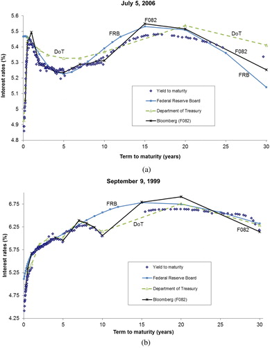
Finally, a convexity problem appears at the long end of the term structure. Non-parametric models usually supply long-term zero-coupon interest rates with implicit non-credible forward rates. It is well known that forward rates are very sensitive to the slope of the yield curve, particularly at the very long end. Therefore, zero-coupon yield curves should be asymptotically flat to provide sensible forward rates.¹⁴ In any event, even when using parametric models such as those of Svensson or Nelson & Siegel, this problem cannot be avoided. Gürkaynak et al. (2007) note that convexity makes it difficult to fit the entire term structure of securities, especially securities of twenty years or more. They maintain that convexity tends to pull down the yields of very long-term securities, giving the yield curve a concave shape at the long end. This reported problem in the FRB database generates three inconsistencies. First, long-term bonds cannot be priced from these zero-coupon yield curves; that is, their prices cannot be replicated from the zero-coupon interest rates estimates provided by the FRB. Second, for sufficiently long maturities, instantaneous forward rates become negative.¹⁵ Third, the β₀ parameter of the Svensson model should capture the long-run level of interest rates. If we consider that estimated values for this parameter lower than 0.01% makes no economic sense, this constraint is saturated in 19% of the dates in the FRB dataset from 1996 to 2017.¹⁶

As a second example, we choose September 9, 1999 (see Panel B of Figure 1) as a clarifying illustration of the problems related with the impact of liquidity on the yield curve estimate. We can see a wide gap in terms of yields to maturities between on-the-run bonds and off-the run bonds.¹⁷ In this case, the data choice is crucial. Depending on this decision, we are actually estimating different interest rates: the spot rates corresponding to the average market liquidity level (F082), the spot rates of the most liquid references (DoT), and the spot rates of the seasoned bonds (FRB). Although the level of these interest rates should be different, it is most likely that the volatility and the correlations among forward rates are also different.

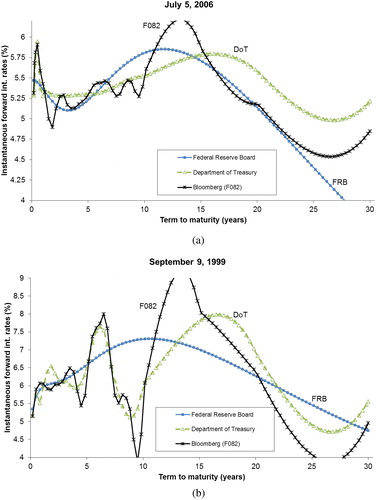
Another important difference among the three datasets can be clearly observed in Panel B of Figure 1. DoT and F082 are far from being smooth curves. Instead, both methods show an overfitting problem for this date. The sawtooth pattern that these two models provide generates serious inconsistencies in the forward rate term structure. Figure 2 plots the implied instantaneous forward rates derived from each dataset for both dates. As we can see, forward rates are extremely sinuous. In addition, the downward shape of the yield curves in the FRB case produces extremely low and even negative forward rates at the long end of the yield curve.

Figure 2. The impact on the instantaneous forward interest rates. The DoT and F082 datasets provide interest rates for certain fixed maturities. We use a simple cubic interpolation technique to build continuous yield curves for these two datasets. For each maturity n, the corresponding instantaneous forward interest rate is proxied by the 1-week rate beginning n years ahead. Panel A. July 5, 2006 Panel B. September 9, 1999

3. Analysis of the time series of alternative yield curve datasets

As we have seen, the three popular zero-coupon yield curve estimates differ considerably in various aspects: the model and methodology employed to fit the yield curves, the market variables used as inputs (prices/yields) and the baskets of assets considered in each sample. Consequently, a direct comparison of goodness of fit between these spot rate datasets is not possible. Previous literature usually compares the ability of different yield curve fitting techniques to replicate bond market prices or to adjust arbitrage-free dynamic term structure models. These authors apply different methods on a unique set of market prices. In our case, the original datasets of market prices used by DoT, FRB and F082 are not available and clearly different. We observe different levels and shapes of the yield curves but there is no way to analyze what the best yield curve are. However, we study the potential consequences of using one of these alternative interest rate datasets on the estimates of other variables that imply using the time series of interest rates: the volatility term structure (VTS) and some correlations between pairs of forward rates. Both variables play a key role in valuation models of interest rate derivatives.

From the three zero-coupon interest rate datasets, we extract spot rates for the 11 maturities reported by the DoT. These maturities range from one month up to 30 years. These spot rates are the input for two alternative methods to estimate the VTS. First, we calculate simple standard deviation measures by using 60-day rolling windows from the log-difference of the value of the spot rates for each maturity. We refer to the resulting annualized volatilities as “historical volatilities.” Second, we examine fitting results of a set of the most common specifications for the well-known family of the conditional volatility models. We consider a standard GARCH (1,1) model because it is traditionally assumed to estimate volatility of daily interest rates (see, e.g., Longstaff & Schwartz, 1992). We also consider the EGARCH model family proposed by Nelson (1991). Among others, Hamilton (1996) and Andersen and Benzoni (2007) have documented that an EGARCH representation for the conditional yield volatility provides a convenient and successful parsimonious model for the conditional heteroskedasticity in short term interest rate time series. According to the Schwarz and Akaike Information Criterion (SIC and AIC respectively), we choose the EGARCH (1, 1) model to estimate interest rate volatility.

Table 3 summarizes descriptive statistics of the VTS estimations from the three interest rate datasets. Both the historical method (panel A) and the conditional method (panel B) produce quite similar values for all the descriptive statistics, except in the short-end of the term structure. The conditional method obtains time series for maturities up to 6-month with higher values for all the statistics, particularly high for the excess of kurtosis. These highly leptokurtic volatilities indicate the presence of extreme values. However, we are not interested in comparing volatility estimation methods but only in examining potential implications of using different interest rate datasets to compute the VTS. The most remarkable outcome is the observed differences among the three datasets in the estimation of the short rate volatilities. There are clear differences in all the reported statistics for maturities of one year or less. Except for the 1-month maturity, the F082 dataset shows higher volatility estimates in this tranche for both the historical and the conditional methods.

Table 3. Descriptive statistics of the Volatility Term Structure.

t	Mean			Std. dev.
	DoT	FRB	F082	DoT	FRB	F082
Panel A: Historical volatility from standard deviations
1-month	1.54	1.25	1.14	2.09	1.72	1.81
3-month	1.32	0.95	1.59	2.06	1.15	2.66
6-month	0.73	0.72	0.83	0.87	0.79	1.14
1-year	0.50	0.54	0.57	0.40	0.44	0.46
2-year	0.51	0.51	0.51	0.35	0.37	0.34
3-year	0.45	0.46	0.47	0.29	0.30	0.30
5-year	0.37	0.36	0.38	0.21	0.21	0.22
7-year	0.31	0.30	0.33	0.16	0.16	0.17
10-year	0.26	0.26	0.28	0.12	0.12	0.12
20-year	0.20	0.20	0.22	0.09	0.09	0.09
30-year	0.20	0.19	0.21	0.09	0.09	0.09
	Skewness			Excess Kurtosis
t	DoT	FRB	F082	DoT	FRB	F082
1-month	1.83	3.19	4.00	2.72	12.89	17.28
3-month	2.18	1.89	2.67	4.22	3.72	7.79
6-month	1.88	1.49	3.00	3.34	1.85	12.05
1-year	0.87	0.76	1.14	0.06	−0.56	1.75
2-year	0.47	0.88	0.53	−0.89	0.42	−0.71
3-year	0.62	0.79	0.70	−0.39	0.02	−0.28
5-year	0.72	0.73	0.73	−0.31	−0.31	−0.31
7-year	0.80	0.80	1.04	−0.08	−0.12	0.84
10-year	0.93	0.93	0.95	0.41	0.26	0.59
20-year	1.05	1.17	1.23	0.58	0.91	1.46
30-year	1.11	1.40	1.53	1.02	2.19	2.94
	Mean			Std. dev.
t	DoT	FRB	F082	DoT	FRB	F082
Panel B: Conditional volatility from EGARCH(1,1)
1-month	2.42	2.30	4.63	2.89	2.28	6.78
3-month	1.77	1.05	1.62	3.40	1.32	3.10
6-month	0.72	0.73	0.86	0.90	0.80	1.24
1-year	0.52	0.55	0.57	0.42	0.44	0.46
2-year	0.52	0.52	0.52	0.35	0.37	0.34
3-year	0.46	0.46	0.47	0.29	0.30	0.30
5-year	0.37	0.36	0.39	0.21	0.20	0.21
7-year	0.31	0.31	0.33	0.16	0.15	0.17
10-year	0.26	0.26	0.28	0.11	0.11	0.11
20-year	0.20	0.20	0.22	0.08	0.08	0.08
30-year	0.17	0.20	0.21	0.11	0.08	0.08
t	Skewness			Excess Kurtosis
	DoT	FRB	F082	DoT	FRB	F082
1-month	1.28	1.61	2.42	0.69	2.65	9.33
3-month	6.39	2.28	3.99	76.36	6.42	20.46
6-month	2.32	1.57	3.73	6.13	2.35	20.01
1-year	1.09	0.78	1.14	0.98	−0.40	2.12
2-year	0.52	0.92	0.63	−0.67	0.72	−0.32
3-year	0.66	0.87	0.78	−0.13	0.49	0.20
5-year	0.73	0.76	0.78	−0.12	−0.05	0.07
7-year	0.79	0.81	1.13	−0.01	0.07	1.43
10-year	0.94	0.98	1.05	0.56	0.57	1.11
20-year	1.11	1.21	1.24	0.84	1.17	1.48
30-year	0.48	1.42	1.59	0.69	2.39	3.58

These tables report daily averages of the volatility term structure (VTS) computed by two alternative methods: annualized standard deviations using 60-day rolling windows from the log-difference of the value of the spot rates (“historical volatilities”) and an EGARCH(1,1) model. As input, we use zero-coupon interest rates from the three daily yield curve datasets (DoT, FRB, F082) during the period from 1996 to 2017 (5,497 trading days and 5,437 volatility estimates).

As we are considering an extremely large daily dataset covering a 22-year period, it would be reasonable to expect the smooth values that we obtain for all the statistics for the maturities higher than 1-year. To test if there are statistically significant differences among the three datasets, we compute parametric and non-parametric test for equality of distributions. Since the VTS series estimated as historical volatilities and as conditional volatilities show similar behavior, we focus on the analysis of historical volatilities.¹⁸ As volatility is computed as an annualized standard deviation using a 60-day rolling window, its time series can present serial autocorrelation problems. Therefore, in the equality tests we use non-overlapping observations, i.e. we consider only one out of every 60 volatility observations (5,497 trading days, 5,437 volatility estimates and 96 observations per sample and maturity).

For each pair of time series, we run a standard t-test of equality of means, a common non-parametric sign test (binomial test) and a signed-ranked test of equality of medians, and the Levene (1960) test of equality of variances. Table 4 shows the results for the pairs DoT versus FRB, F082 versus FRB, and DoT versus F082, where the first dataset is called “X” and the second one “Y”. We compute the “X/Y ratio” at time t by dividing the volatility level from the dataset X at time t by the corresponding volatility from the Y dataset at time t. The table shows average X/Y ratio, the percentage of times the ratio is higher than the unity. Also, we compute the t-test, the sign test, the signed-ranked test where the null hypothesis is that the X/Y ratio is equal to unity, i.e., there is no significant difference between the volatility level of both the X and the Y datasets. We also compute the Levene test of equal variances in each pair of volatility series.

Table 4. Test results for differences in VTS.

t	Ratio DoT / FRB
	Mean	% >1.0	t-test	Sign test	Signed-rank test	Variance test
1-month	1.90	74	5.44**	4.01**	4.76**	5.83*
3-month	1.31	56	2.86**	1.06	2.32*	11.76**
6-month	1.04	52	1.11	0.31	0.51	0.02
1-year	0.97	43	−1.30	1.33	1.48	0.64
2-year	1.01	45	1.07	0.92	0.02	0.00
3-year	0.98	23	−2.56*	3.61**	3.54**	0.01
5-year	1.00	39	−0.56	2.14*	2.65**	0.15
7-year	1.01	46	1.26	0.71	0.05	0.20
10-year	1.00	57	0.41	1.33	1.37	0.01
20-year	1.02	69	3.01**	3.57**	3.74**	0.15
30-year	0.98	30	−1.92	3.42**	2.93**	0.08
	Ratio F082 / FRB
t	Mean	% >1.0	t-test	Sign test	Signed-rank test	Variance test
1-month	2.31	81	6.22**	4.18**	5.02**	0.36
3-month	1.51	52	3.74**	0.14	1.11	17.89**
6-month	1.21	71	2.98**	2.74**	3.85**	2.09
1-year	1.10	90	4.62**	5.34**	5.39**	0.01
2-year	1.04	77	2.90**	3.61**	4.81**	0.46
3-year	1.03	77	3.83**	3.61**	3.88**	0.03
5-year	1.07	90	9.31**	5.34**	5.32**	0.34
7-year	1.09	94	10.58**	5.92**	5.66**	0.48
10-year	1.11	92	7.82**	5.63**	5.51**	0.06
20-year	1.12	92	8.87**	5.63**	5.70**	0.01
30-year	1.13	77	4.91**	3.61**	4.06**	0.01
	Ratio DoT / F082
t	Mean	% >1.0	t-test	Sign test	Signed-rank test	Variance test
1-month	0.89	10	−1.01	5.34**	5.35**	0.61
3-month	1.18	23	1.48	3.61**	3.87**	0.11
6-month	0.98	17	−0.40	4.47**	4.38**	1.55
1-year	0.92	10	−3.48**	5.34**	5.54**	0.80
2-year	−1.02	10	−1.02	5.34**	5.70**	0.65
3-year	0.96	15	−4.91**	4.76**	5.09**	0.09
5-year	0.94	8	−10.09**	5.63**	5.89**	0.04
7-year	0.92	2	−11.38**	6.50**	5.95**	0.07
10-year	0.91	4	−10.27**	6.21**	5.86**	0.02
20-year	0.91	4	−9.48**	6.21**	5.99**	0.07
30-year	0.89	3	−8.89**	4.83**	4.56**	0.00

Volatility term structure (VTS) computed by annualized simple standard deviation measures using 60-day rolling windows from the log-difference of the value of the spot rates (“historical volatilities”). As the input, we use zero-coupon interest rates from three yield curve datasets (Department of the Treasury, DoT; Federal Reserve Board, FRB; Bloomberg, F082) during the period from January 1996 to December 2017. In these tests we use non-overlapping observations from the VTS time series, i.e. we consider only one out of every 60 volatility observations (5,497 trading days, 5,437 volatility estimates and 96 observations per sample).

The X/Y ratio is defined as the mean volatility for the X dataset divided by the corresponding mean for the Y dataset. The hypothesis that the mean of the X/Y ratio is equal to unity is tested using a standard t-test. A standard sign test is used to test that the proportion of X/Y ratios higher than unity is equal to the proportion of ratios lower than unity, which is equal to 0.5. The Levene statistic is used to test the equality of variances between X and Y.

** and * indicate significance at 1% and 5% level, respectively, in a two-tailed test.

Table 4 shows clear evidence of statistically significant discrepancies for most maturities. The different behavior of the volatility time series obtained from the F082 dataset is significant from a statistical point of view for nearly the entire maturity spectrum. Differences in the volatility level of the zero-coupon interest rates computed from the FRB or the DoT datasets are only significant in the short end of the yield curve (1- and 3-month), in the central range of maturities (3- and 5-year), and in the long end (20- and 30-year). The null hypothesis of equal means and equal medians between DoT and FRB cannot be rejected for key maturities of the VTS, i.e. maturities from 6-month to 2-year and maturities from 7- to 10-year. In the case of the variance of the volatility, we also observe statistically significant differences among the three interest rate datasets for the shortest maturities. These dissimilar behaviors observed in the VTS computed from the three datasets have relevant implications for practitioners, academics, supervisors, and policy makers. As mentioned above, VTS is a key variable in a multitude of studies, in fields such as financial economics, macroeconomics and monetary policy. For instance, interest rate models are calibrated to fit the model parameters to the VTS market data. These models are used for pricing or assessing any fixed income securities and their derivatives. In addition, Value-at-Risk and Expected Shortfall calculations in fixed income portfolios are extremely sensitive to the VTS and the correlations among different maturities.

We also proceed to a preliminary analysis of the existence of a volatility spillover among these three datasets. There are at least two reasons why volatility changes in one data set may precede changes in other datasets: differences in the liquidity of the assets considered to estimate zero coupon bonds (on-the-run bills and bonds for DoT, second or further off-the-run bonds for FRB, and all bonds for F082), and the different degrees of flexibility of the functional form employed to estimate the yield curve. Moreover, this different degree of flexibility can be more acute in the different tranches of the yield curve (e.g., the weighted Svensson model used by FRB is forced to better adjust short-term zero-coupon bonds at the cost of poorer long-term adjustment).

To explore these potential indirect effects, we estimate a three-dimensional VAR model in which the variables examined are the daily changes in the volatility of interest rates for a given maturity obtained from the three sets of interest rates (FRB, DoT and F082).¹⁹ Specifically, we consider the volatilities estimated through the E-GARCH model, described in Section 3, for four of the main interest rate maturities: 3 months, and 2, 5 and 10 years.

The results suggest that cross-dataset volatility spillovers appear mainly in the medium and long end of the term structure.²⁰ For short maturities, we only find a Granger-causality positive relationship from FRB estimates to F082 dataset. On the contrary, for medium and longer maturities the relationships are more entangled. In this case, changes in the volatility of more flexible models precede changes in the volatility of more rigid ones. The most robust result we find is a positive Granger-causality relationship from F082 data set to both FRB and DoT and from DoT estimates to FRB. Other relationships appear for some specific maturities, but they are not present for others. Thus, we can conclude that the use of a particular functional form to estimate the yield curve may be the origin of the leading-lag relationships found in interest rate volatility estimates, a result that may depend on the tranche of the yield curve and the flexibility of the model used to estimate that yield curve.

We also examine effects of using alternative interest rate datasets on the correlations between pairs of forward rates. A popular approach to modeling term structure dynamics computes the forward rate process directly, using the initial historical forward rate volatilities as an input. The properties of the correlation matrix of instantaneous forward rates for different maturities is crucial in these models. Forward rates also play a key role in many other financial issues, such as pricing financial products where correlations among forward rates are crucial (e.g., interest rate caps and swaptions), and in analyses of market expectations about future short-term interest rates. The empirical behavior of interest rates implies that the long-term forward rates should be less volatile than short-term forward rates. Desirable properties of any yield curve are that it should produce a smooth forward rate curve, which converges to a fixed limit as maturity increases. Forward rates are highly sensitive to the shape of the yield curve, particularly at the very long end. The intuition says that the correlation between short-term forward rates should be lower than the correlation between long-term forward rates. Economic rationality suggests an almost perfect positive correlation between long-term forward rates. Under the assumption that forward rates reflect expectations about future short-term interest rates, agents should perceive similar values for the interest rates for different long horizons.²¹

We compute time series of pairwise correlation coefficients by using 60-day rolling windows between three pairs of several year-ahead forward rates with a six-month tenor. We consider maturity pairs in the short-end, in the medium-term, and in the long-end of the yield curve. In particular, we examine the correlation between the six-month spot rate, R_0.5, and the one-year ahead forward rate with a half-year tenor, F_1,1.5, i.e. ρ(R_0.5; F_1,1.5), the correlation between the 2- and the 5-year forward rate, ρ(F_2,2.5; F_5,5.5), and the correlation between the 10- and the 29.5-year forward rate ρ(F_10,10.5; F_29.5,30).

Panel A of Table 5 summarizes statistics of pairwise correlations from daily contemporaneous forward rates on the three time horizons. The mean values of the correlations in the shortest and the medium-term maturities are quite similar for the three interest rate datasets used to compute the forward rates. The main difference is observed in the long-end of the yield curve. For this time horizon, the “desirable” result should be values close to the unity because the expected asymptotically flat forward rate curve. The highest correlation is obtained from DoT dataset (ρ = 0.7), but this value is almost two and three times the mean values obtained from FRB and F082 respectively. In fact, one third of the long-term correlations computed from the F082 are negative (more than 13 percent in the case of the FRB).²² In addition, the standard deviation of these correlations is much higher in the case of FRB and F082. The DoT dataset is the only one to support the intuition of increasing correlations between forward rates as maturity increases. Thus, this result for the FRB and F082 datasets is far from the desirable property of correlation coefficients to be close to the unity for long maturities.

Table 5. Summary statistics of correlations between forward rates.

t	Mean			Std. dev.
	DoT	FRB	F082	DoT	FRB	F082
Panel A: Descriptive statistics
R0.5 ; F1,1.5	0.444	0.445	0.467	0.229	0.412	0.218
F2,2.5 ; F5,5.5	0.722	0.867	0.711	0.119	0.067	0.157
F10,10.5 ; F29.5,30	0.702	0.375	0.274	0.138	0.332	0.482
	Skewness			Excess Kurtosis
t	DoT	FRB	F082	DoT	FRB	F082
R0.5 ; F1,1.5	−0.316	−0.722	−0.551	−0.792	−0.827	−0.321
F2,2.5 ; F5,5.5	−1.027	−1.320	−0.966	0.919	2.270	0.629
F10,10.5 ; F29.5,30	−0.921	−0.311	−0.369	0.601	−0.570	−1.184
	Ratio (DoT + 1) / (FRB + 1)
t	Mean	% >1.0	t-test	Sign test	Signed-rank test	Variance test
Panel B: Test results for differences in correlations between forward rates
R0.5 ; F1,1.5	1.07	44	2.19*	1.12	0.84	54.29**
F2,2.5 ; F5,5.5	0.92	7	−12.79**	8.27**	8.33**	24.02**
F10,10.5 ; F29.5,30	1.31	83	6.73**	5.70**	6.65**	67.44**
	Ratio (DoT + 1) / (F082 + 1)
t	Mean	% >1.0	t-test	Sign test	Signed-rank test	Variance test
R0.5 ; F1,1.5	0.99	50	−0.33	−0.10	0.16	1.11
F2,2.5 ; F5,5.5	1.02	49	1.55	0.10	0.59	8.88**
F10,10.5 ; F29.5,30	1.64	75	4.88**	4.33**	6.01**	144.80**
	Ratio (F082 + 1) / (FRB + 1)
t	Mean	% >1.0	t-test	Sign test	Signed-rank test	Variance test
R0.5 ; F1,1.5	1.11	40	2.64**	1.94	0.34	67.73**
F2,2.5 ; F5,5.5	0.92	8	−10.14**	8.06**	8.23**	55.97**
F10,10.5 ; F29.5,30	0.96	43	−1.02	1.14	1.77	20.69**

Pairwise correlation coefficients from daily forward rates using 60-day rolling windows. They are six-month forward rate starting at time 0, 1, 2, 5, 10 and 29.5 (F_0,0.5 = R_0.5, F_1,1.5, F_2,2.5, F_5,5.5, F_10,10.5, and F_29.5,30 respectively). For instance, F_5,5.5 is the 5-year ahead forward rate with a half-year tenor. As the input, we use zero-coupon interest rates from the three yield curve datasets (Department of the Treasury, DoT; Federal Reserve Board, FRB; Bloomberg, F082) during the period from January 1996 to December 2017 (5,497 trading days). Panel A reports summary statistics for the full sample of 5,437 daily observations of each forward correlation. Panel B shows results of equality tests in which we use non-overlapping observations from the daily correlation time series, i.e. we consider only one out of every 60 correlation observations (96 observations per sample). As the correlation coefficient can have values ranging from +1 to –1, the X/Y ratio is defined as the mean correlation coefficient for the X dataset plus one divided by the corresponding mean for the Y dataset plus one. The hypothesis that the mean of the X/Y ratio is equal to unity is tested using a standard t-test. A standard sign test is used to test that the proportion of X/Y ratios higher than unity is equal to the proportion of ratios lower than unity, which is equal to 0.5. The Levene statistic is used to test the equality of variances between X and Y.

** and * indicate significance at 1% and 5% level, respectively, in a two-tailed test.

Panel B of Table 5 reports formal tests for differences in correlations between forward rates obtained from alternative interest rate datasets. In this case, the pairwise correlations are computed using three-month non-overlapping periods (96 periods).²³ The null hypotheses of equal mean, median and variance between forward correlations are rejected in most cases. These hypotheses cannot be rejected for the comparison among DoT and F082, for both short- and medium-term maturities, and among FRB and F082 at the longer end. Besides these exceptions, results of these analyses corroborate previous findings. There are statistically significant differences in the behavior of forward rates when different interest rate datasets are used. Using a different interest rate dataset as input can affect the pricing of interest rate derivatives. For instance, Brigo and Fabio (2001) and Rebonato (2002) find that an increase in the average correlation between the percentage changes in discrete forward rates increases the valuation of swaptions.

4. The relevance of the use of alternative yield curve estimations

The expectations hypothesis has a central role in term structure theory. An extensive financial economics literature has tested whether the expectations hypothesis holds. Most studies have frequently rejected the expectations hypothesis. However, results vary from one study to the next depending on the methodology, the maturity spectrum, the frequency of the data, the sample period, and the source of the interest rates. The latter conditioning factor is related with our study. In this sense, Longstaff (2000) highlights that negative findings obtained in previous studies result from using Treasury bill rates. The apparent term premium is influenced for other security-specific features such as their liquidity. Longstaff finds support for the expectations hypothesis from repo data, considering repo rates as measures of the short-term riskless term structure. Other authors, such as Downing and Oliner (2007) and Brown, Cyree, Griffiths, and Winters (2008), obtain the opposite result from commercial paper interest rates.

To test the expectations hypothesis is a relevant exercise to illustrate the relevance of choosing one among alternative yield curve datasets. As Longstaff (2000) points out, Treasury bill yields often exhibit specialness and idiosyncratic variations. It is not uncommon for researchers to exclude bills from their analyses of the term structure of interest rates. The DoT is the only examined dataset to consider Treasury bills. Also, it only includes on-the-run bills which are the focus of specialness. Both the FRB and the F082 exclusively consider Treasury notes and bonds. In addition, the lowest maturities range from 1-month in the case of DoT and from 3-month in the case of the F082.

In this section, we replicate the result of a simple expectations hypothesis test. We only attempt to analyze the impact of using one or another yield curve dataset on a widely studied test. This study does not claim to provide a comprehensive and detailed analysis of the expectations analysis but instead aims to highlight the implications of using different samples of rates. Therefore, we merely reproduce the classical Campbell’s (1995) test for our alternative yield curve datasets. As a slight robustness improvement, we use instrumental variables to address the problem of measurement error for long-term interest rate (see, e.g., Campbell & Shiller, 1991). We do not attempt to find evidence supporting or rejecting the theory; instead, we only attempt to illustrate the possible implications of considering one or another yield curve dataset. We run all the regressions using the same methodology, the same maturity spectrum, the same frequency of the data, the same sample period, but using the three alternative external interest rate datasets.

The inputs of the tests are prepared following the detailed description of Campbell (1995). We calculate continuously compounded yields by using one month as the basic time unit.²⁴ The yield spread of a bond is defined as the difference between its yield and the short rate. As the short rate, Campbell (1995) uses the yield of a 1-month Treasury bill. Because the DoT reports yields of on-the run securities for several fixed maturities, our actual 1-month yield is proxied by the 1-month yield reported by the DoT dataset. The excess return is calculated as the difference between bond returns and the short yield. The excess return is also the yield spread less (m-1) times the change in the bond yield, where m is the maturity in months.

The expectations hypothesis implies that excess returns of long bonds over short bonds are zero on average, as required by the pure expectations hypothesis. The first row of Table 1 (page 135) in Campbell (1995) checks whether the excess return of long bonds over short bonds has a zero mean.²⁵ Table 6 reports the results of replicating the Campbell’s original Table 1 by using the three yield curve datasets (Panels A, B and C) and reproduces the Campbell’s results (panel D). Instead of the hump-shaped excess returns observed in Campbell, we obtain that the excess return increases with maturity. Most relevant for our analysis are the important differences among datasets in the estimation of excess returns for the 10-year maturity and the maturities shorter than 6 months. The mean excess return from the FRB dataset is two and three times higher than the obtained from the other datasets in the short end of the curve. As expected, excluding bills produces important differences with respect to other datasets. However, the largest difference in absolute terms among datasets is observed for the 10-year maturity. The omission of on-the-run bonds in the FRB basket of assets provides larger excess returns in this particular analysis.

Table 6. Replication of “Table 1 Means and Standard Deviations of Term Structure Variables” (Campbell, 1995, p. 135).

	Long bond maturities (months)
Variable	2	3	6	12	24	48	120
Panel A. Department of Treasury (DoT)
Excess return	0.074	0.141	0.280	0.417	0.767*	1.261*	2.381*
	(0.219)	(0.407)	(1.021)	(2.462)	(6.477)	(14.34)	(33.32)
Change in yield	−0.002	−0.001	−0.001	−0.001	−0.003*	−0.005*	−0.007*
	(0.254)	(0.213)	(0.210)	(0.228)	(0.281)	(0.304)	(0.279)
Yield spread	0.073	0.140	0.274	0.401	0.697*	1.023*	1.528*
	(0.119)	(0.226)	(0.341)	(0.391)	(0.569)	(0.785)	(1.182)
Panel B. Federal Reserve Board (FRB)
Excess return	0.235	0.251	0.313	0.460	0.751*	1.275*	2.643
	(0.307)	(0.434)	(0.957)	(2.488)	(6.360)	(14.26)	(32.42)
Change in yield	−0.001	−0.001	−0.001	−0.002	−0.003*	−0.005*	−0.008
	(0.225)	(0.206)	(0.199)	(0.229)	(0.276)	(0.301)	(0.271)
Yield spread	0.236	0.251	0.308	0.440	0.675*	1.018*	1.732*
	(0.240)	(0.264)	(0.337)	(0.426)	(0.555)	(0.807)	(1.273)
Panel C. Bloomberg (F082)
Excess return	0.000	0.098	0.277	0.443	0.722*	1.278*	2.395*
	(0.300)	(0.402)	(1.002)	(2.566)	(6.454)	(14.35)	(32.65)
Change in yield	−0.002	−0.001	−0.001	−0.002	−0.003*	−0.005*	−0.007*
	(0.247)	(0.203)	(0.205)	(0.236)	(0.280)	(0.303)	(0.273)
Yield spread	−0.001	0.096	0.271	0.421	0.647*	1.023*	1.512*
	(0.201)	(0.240)	(0.363)	(0.437)	(0.577)	(0.809)	(1.239)
Panel D. Original Campbell’s Table 1
Excess return	0.379	0.553	0.829	0.862	0.621	0.475	−0.234
	(0.640)	(1.219)	(2.950)	(6.203)	(11.29)	(19.32)	(36.77)
Change in yield	0.014	0.014	0.014	0.014	0.014	0.014	0.013
	(0.591)	(0.575)	(0.569)	(0.546)	(0.486)	(0.408)	(0.307)
Yield spread	0.196	0.324	0.569	0.761	0.948	1.141	1.358
	(0.210)	(0.301)	(0.437)	(0.594)	(0.799)	(1.013)	(1.234)

Continuously compounded yields calculated from zero-coupon interest rates from the three external yield curve datasets (Department of the Treasury, DoT; Federal Reserve Board, FRB; Bloomberg, F082) and from our own yield curve estimates, applying the weighted Svensson to the four different datasets from GovPx asset prices. The sample period ranges from January 1994 to December 2017. The yield spread is defined as the difference between the bond yield and the short yield. The excess return is calculated as the difference between the return on a bond and the short yield. The short yield is proxied by the 1-month yield reported by the DoT dataset. Standard deviations are shown in parentheses.

*indicates significance at 5% level in a two-tailed test.

Campbell footnote: “Source: Author's calculations using estimated monthly zero-coupon yields, 1952–1991, from McCulloch and Kwon (1993). The data are measured monthly, but expressed in annualized percentage points. Each row shows the mean of the variable, with the standard deviation below in parentheses. Excess returns and yield spreads are measured relative to 1-month Treasury bill rates.”

Campbell (1995) also analyses whether excess returns on long bond over short bonds are unforecastable over the life of the short bond. According to the experiment design, the expectations hypothesis holds if the slope coefficients from the regressions of long rate changes on a constant and the long-short yield spread should be one (first row of the Campbell’s original Table 2, page 139). Panels A to C in our Table 7 replicate these tests using the three datasets. Panel D reproduces Campbell’s (1995) original Table 2. The differences among the results obtained from the alternative yield curves can be observed in all maturities in both level and statistical significance. Tests using the DoT dataset provide markedly different results from those obtained using the other yield curves, especially in the case of the shortest maturity (2-month) and for the 2- and 4-year.

Table 7. Replication of “Table 2 Regression Coefficients” (Campbell, 1995, p.139).

	Long bond maturities (months)
Variable	2	3	6	12	24	48	120
Panel A. Department of Treasury (DoT)
Short-run changes	1.207*	0.984*	1.599*	1.852*	−0.064	−1.981	−2.873
in long yields	(0.296)	(0.289)	(0.452)	(0.807)	(1.286)	(1.862)	(2.649)
Long-run changes	2.919*	1.372*	1.222*	1.528*	0.970*	0.943*	−0.074
in short yields	(0.751)	(0.318)	(0.181)	(0.216)	(0.259)	(0.209)	(0.126)
Panel B. Federal Reserve Board (FRB)
Short-run changes	0.301	0.652*	1.299*	1.490*	−1.997	−0.042	−2.872
in long yields	(0.177)	(0.248)	(0.389)	(0.741)	(1.787)	(0.038)	(2.370)
Long-run changes	1.397*	1.193*	1.128*	1.243*	1.086*	0.978*	−0.069
in short yields	(0.457)	(0.276)	(0.179)	(0.209)	(0.271)	(0.202)	(0.142)
Short-run changes	0.202	0.757*	1.085*	1.349	−2.059	−0.044	−2.299
in long yields	(0.273)	(0.265)	(0.368)	(0.737)	(1.799)	(0.038)	(2.463)
Long-run changes	0.949	1.222*	1.030*	1.185*	1.009*	0.995*	−0.069
in short yields	(0.671)	(0.311)	(0.162)	(0.202)	(0.256)	(0.201)	(0.156)
Panel D. Original Campbell’s Table 2
Short-run changes	0.019	−0.135	−0.842	−1.443	−1.432	−2.222	−4.102
in long yields	(0.194)	(0.285)	(0.444)	(0.598)	(0.996)	(1.451)	(2.083)
Long-run changes	0.510	0.473	0.301	0.253	0.341	0.435	1.311
in short yields	(0.097)	(0.149)	(0.147)	(0.210)	(0.221)	(0.398)	(0.120)

Continuously compounded yields calculated from zero-coupon interest rates from the three external yield curve datasets (Department of the Treasury, DoT; Federal Reserve Board, FRB; Bloomberg, F082) and from our own yield curve estimates, applying the weighted Svensson to the four different datasets from GovPx asset prices. The sample period ranges from January 1994 to December 2017. The yield spread is defined as the difference between the bond yield and the short yield. The excess return is calculated as the difference between the return on a bond and the short yield. The short yield is proxied by the 1-month yield reported by the DoT dataset. Standard deviations are shown in parentheses.

*indicates significance at 5% level in a two-tailed test. Campbell footnote: “Source: Author's calculations using estimated monthly zero-coupon yields, 1952–1991, from McCulloch and Kwon (1993). Each row shows a regression coefficient β, with the standard error below in parentheses. Each coefficient should be one if the expectations hypothesis holds. The regression in the first row is $$y_{m-1,t+1}-y_{m,t}=\alpha +\beta \left(y_{m,t}-y_{1,t}\right)/\left(m-1\right)$$ where m is long bond maturity in months. The regression in the second row is $$\sum _{i=1}^{m-1}\frac{y_{1,t+i}}{m-1}-y_{1,t}=\mathrm{\alpha }+\beta \left(\frac{m-1}{m}\right)\left(y_{m,t}-y_{1,t}\right)$$

The standard error in the second row is corrected for serial correlation in the error term of the regression.”

In summary, the results obtained in this section suggest that the conclusions of a simple test as those conducted by Campbell (1995) can differ significantly depending upon the yield curve estimates used to perform the test. The differences observed may affect both the size of the parameters estimations and its statistical significance. These differences go beyond the inclusion/exclusion of Treasury bills. Most discrepancies affect medium and long maturities.

5. Conclusions

This paper reports on the nature of alternative zero-coupon yield curve datasets and on how such datasets can lead to somewhat different results for some common purposes in financial economics. It is somewhat reassuring that for many of the instances we examine, the results are generally robust for the three datasets. But in some cases, the empirical results are quite sensitive to the yield curve data.

The most obvious difference among datasets is the liquidity of the considered securities. The on/off-the-run phenomenon is well-known in the literature. The basket of assets used as input for the DoT estimates includes only on-the-run securities. Instead, the FRB excludes all the bills and the on-the-run and first-off-the-run bonds. The F082 includes all the outstanding bills and bonds. However, there are other relevant aspects that may generate different behavior and shapes on the yield curves. The three data providers use different parametric and non-parametric models in the fitting process. In addition, they consider quotes, end-of-day prices, or yields to maturity.

In this paper, we examine different properties of the yield curves and their indirect implications on two relevant variables: the resulting volatility term structure and the correlations between forward rates. The outcomes suggest that even if bond prices are replicated accurately using any of the three popular datasets examined, the impact on other variables can be remarkable, especially at both ends of the yield curve. Differences in volatilities primarily affect the short end of the yield curve; moreover, the discrepancies are large with respect to correlations between long-term forward rates.

Finally, we study the extent to which the choice among alternative yield curve datasets matters for the results of a simple tests of the expectations hypothesis. The outcomes clearly indicate that when short rates (less than one year) or long rates (more than ten years) are involved, the results may differ significantly depending upon the set of yield curves used to test the expectations hypothesis. Excluding bills is not the only source of discrepancies among datasets.

In general, the DoT dataset performs well in the short end of the yield curve. It should be a good input for institutional investors interested on pricing liquid short-term assets. Moreover, for valuating interest rate derivatives and for monetary economics purposes, the smooth on-the-run yield curve obtained by the DoT provides forward rates consistent with theory. With respect to financial data users interested on pricing bonds and other medium and long-term instruments with a “regular” liquidity level, the FRB dataset is a good choice. The information reported by the FRB allows to compute zero-coupon rates for any maturity obtaining a continuous yield curve with flexible and reliable shape. In addition, their low volatility levels for most maturities are a desirable property for risk management purposes. Finally, the F082 dataset provided by Bloomberg performs a “too” good fitting for all the maturity spectrum and shows the “average” liquidity level in the US bond market. In some cases, this overfitting may show some important relationships that could be modeled and are overlooked by the other datasets. In other cases, it simply fits to the noise present in the prices. These yield curves provide an accurate view of the current full market situation.

In conclusion, we can state that choosing one or another zero-coupon interest rate dataset can lead to empirical results that can differ significantly. The dataset choice may matter. When empirical results are sensitive to the dataset, researchers, traders, portfolio managers, policymakers, etc. should be cautious about selecting the most appropriate dataset or even about accepting those particular results or the empirical method that led to those results. Final users of the yield curve data should check the empirical results against alternative datasets, or at least they should defend the use of one of them depending on their respective applications.

Additional information

Funding

This work was supported by the Spanish Ministerio de Economía, Industria y Competitividad (ECO2017-89715-P).

Notes

1 Current and historical H.15 data are available on the Board's Data Download Program (DDP) at www.federalreserve.gov/datadownload/Choose.aspx?rel=H15.

2 US DoT’s website address is: https://www.treasury.gov/resource-center/data-chart-center/interest-rates/Pages/TextView.aspx?data=yield.

3 The website address of the FRB dataset is: https://www.federalreserve.gov/econresdata/feds/2006/index.htm.

4 According to the Bank Of International Settlements, (2005), nine out of thirteen central banks used either the Nelson and Siegel, (1987) or the extended version suggested by Svensson, (1994) for estimating the term structure of interest rates.

5 They recognize that the function employed could also result in unstrippable zero curves and negative forward rates. See M. Lee, International Bond Market Conference 2007, Taipei.

6 Bloomberg terminal mentions: “The yield curve is built daily with bonds that have either Bloomberg Generic (BGN) prices, supplemental proprietary contributor prices or both. The bonds are subject to option-adjusted spread (OAS) analysis and the curve is adjusted to generate a best fit. (…) Bloomberg Generic Price (BGN) is Bloomberg’s market consensus price (…) Bloomberg Generic Prices are calculated by using prices contributed to Bloomberg and any other information that we consider relevant.”

7 Coupon bias represents the difference between the yield to maturity of a coupon-bearing bond and the zero-coupon interest rate with the same term to maturity. The yield to maturity for a coupon-bearing bond is a sort of weighted average of the rates associated with the term to maturity of each cash flow generated by the coupon-bearing bond. The steeper the term structure or the larger the coupon, the greater the coupon bias. In referring to forward bias, Livingston and Jain, (1982) illustrate the different behavior for long maturities of the implied forward rates obtained from the par yields and the actual forward rate computes from zero-coupon interest rates.

8 Treasury does not accept negative yields in Treasury nominal security auctions.

9 See, e.g., Amihud and Mendelson, (1991), Duffie, (1996), Warga, (1992), Longstaff, (2000), Krishnamurthy, (2002), Goldreich et al., (2005), and Vayanos and Weill, (2008).

10 See, e.g., Fleming, (2000), Pasquariello and Vega, (2009), Graveline and McBrady, (2011) and Fontaine and Garcia (2012).

11 In fact, the BIS (2005) comments that most central banks exclude part of the maturity range for which debt instruments are available. For instance, certain central banks consider only the interval from one to ten years.

12 Our GovPX sample ranges from January 1994 to December 2006. The transaction data available until May 2001 include the last trade time, size, and side (buy or sell), the price (or yield in the case of bills), and the aggregate volume (volume in millions traded from 6 pm on the previous day to 5 pm). The quote data used from June 2001 include the best bid and ask prices (or discount rate actual/360 in the case of bills) and the mid-price and mid-yield (actual/365).

13 Callable bonds are excluded. When two securities have the same remaining maturity, only the youngest one is considered.

14 If we assume that forward rate contains information regarding economic agents’ expectations about future interest rates, it would be sensible to assume that the 30-year forward rate should be similar to the 31-year forward rate.

15 Gürkaynak et al.,(2007) recognize that the Svensson specification “assumes that forward rates eventually asymptote to a constant. The downward tilt to forward rates at long horizons is an important characteristic of the U.S. yield curve; for example, the instantaneous forward rate ending 25 years ahead has continuously been below the instantaneous forward rate ending 20 years ahead for the past decade.”

16 Please, note that negative values for this parameter are not allowed. Theoretically, this parameter should be positive as it is the asymptotic value of instantaneous forward rate when the term to maturity approaches infinity.

17 The period from fall 1998 to the end of 1999 is characterized by several episodes of flights-to-quality. It has been suggested that the Year 2000 bug (Y2K) effect was one of the triggers.

18 The results obtained from EGARCH volatilities can be requested from the authors.

19 We apply the Augmented Dickey-Fuller Test, the Phillips-Perron Test, and the Kwiatkowski-Phillips-Schmidt-Shin test to check the stationarity of volatility changes rejecting the hypothesis of existence of a unit root.

20 To check the statistical significance of the model, we applied the VAR – Granger - causality Wald test using Eviews 7. All statistical results are available upon request.

21 Forward rates may embed term premiums increasing with maturity. Our analysis examines the possible impact of using one or another interest rate dataset on the correlation between forward rates in three time horizons. For each correlation, we compare its behavior in each dataset, so the results of our analysis should not be related to the impact of term premiums that are the same for all the three datasets. However, these premiums could affect the order of magnitude of the differences in correlations between datasets for different time horizons.

22 In the case of the F082 dataset, this result could be caused by the fitting method of the yield curve between 20- and 30-year maturities. First, there are only a few number of observations with a maturity longer than ten years. Second, F082 estimation at the long end of the curve merely consists of a linear interpolation between 20- and 30-year interest rates without a real estimation of intermediate rates. Thus, F_10,10.5 and F_29.5,30 become extremely dependent of the position of the 20-year rates. If it is high (with respect to 10- and 30-year rates) it makes F_10,10.5 go up while making F_29.5,30 go down. Inversely, if the 20-year rate is low (compared with 10- and 20-year rates), F_10,10.5 will decrease while F_29.5,30 will rise.

23 As the correlation coefficient can have values ranging from +1 to –1, the X/Y ratio is defined as the mean correlation coefficient for the X dataset plus one divided by the corresponding mean for the Y dataset plus one.

24 The DoT provides market yields that are either investment yields or bond-equivalent yields. They use simple interest and day count convention actual/actual. We recalculate this yield as a continuously compound interest rate. No 1-month rates are available in this dataset until August 1, 2001. Prior to this date, we estimate the corresponding interest rate by using cubic interpolation.

25 The data in Table 7 are reported in annualized percentage points, i.e., the natural monthly variables are multiplied by 1,200.

References

- Amihud, Y., & Mendelson, H. (1991). Liquidity, maturity and the yield on U.S. treasury securities. The Journal of Finance, 46(4), 1411–1425. doi:10.2307/2328864
- Andersen, T. G., & Benzoni, L. (2007). Do bonds span volatility risk in the U.S. treasury market? A specification test for affine term structure models (Working Paper No. W12962). NBER.
- Andreasen, M. M., Christensen, J. H. E., & Rudebusch, G. D. (2017). Term structure analysis with big data (Working Paper Series, 01). Federal Reserve Bank of San Francisco, doi:10.24148/wp2017-21
- Ang, A., & Piazzesi, M. (2003). A no-arbitrage vector autoregression of term structure dynamics with macroeconomic and latent variables. Journal of Monetary Economics, 50(4), 745–787. doi:10.1016/S0304-3932(03)00032-1
- Backus, D. K., Gregory, A. W., & Zin, S. E. (1989). Risk premiums in the term structure: Evidence from artificial economies. Journal of Monetary Economics, 24(3), 371–399.
- Baig, T., & Goldfajn, I. (1999). Financial market contagion in the Asian crisis. IMF Working Papers, 46(2), 167–195. doi:10.5089/9781451857283.001
- Bank Of International Settlements, (2005). Zero-coupon yield curves: Technical documentation. BIS Papers, No. (25 October)
- Barnejee, S., & Graveline, J. J. (2013). The cost of short-selling liquid securities. The Journal of Finance, 68, 637–664. doi:10.1111/jofi.12009
- Black, F., Derman, E., & Toy, W. (1990). A one-factor model of interest rates and its application to treasury bond options. Financial Analysts Journal, 46(1), 33–39. doi:10.2469/faj.v46.n1.33
- Bliss, R. R. (1996). Testing term structure estimation methods. Advances in Futures and Options Research, 9, 197–231.
- Bolder, D. J., & Gusba, S. (2002). Exponentials, polynomials, and fourier series: More yield curve modelling at the bank of Canada (Working Paper No. 2002-29). Canada: Bank of Canada.
- Bolder, D. J., Johnson, G., & Metzler, A. (2004). An empirical analysis of the Canadian term structure of zero-coupon interest rates (Working Paper No. 2004-48). Canada: Bank of Canada.
- Brigo, D., & Fabio M. (2001). “Interest rate models: Theory and practice”. Berlin: Springer Finance.
- Brown, C. G., Cyree, K. B., Griffiths, M. D., & Winters, D. B. (2008). Further analysis of the expectations hypothesis using very short-term rates. Journal of Banking & Finance, 32(4), 600–613. doi:10.1016/j.jbankfin.2007.04.026
- Campbell, J. Y. (1995). Some lessons from the yield curve. Journal of Economic Perspectives, 9(3), 129–152. doi:10.1257/jep.9.3.129
- Campbell, J., & Shiller, R. (1991). Yield spreads and interest rates movements: A bird’s eye view. The Review of Economic Studies, 58(3), 495–514. doi:10.2307/2298008
- Cochrane, J. H., & Piazzesi, M. (2002). The fed and interest rates-a high-frequency identification. American Economic Review, 92(2), 90–95. doi:10.1257/000282802320189069
- Corsi, F., Mittnik, S., Pigorsch, C., & Pigorsch, U. (2008). The volatility of realized volatility. Econometric Reviews, 27 (1–3), 46–78. doi:10.1080/07474930701853616
- Cox, J. C., Ingersoll, J. E., Jr., & Ross, S. A. (1985). An intertemporal general equilibrium model of asset prices. Econometrica, 53(2), 363–384. doi:10.2307/1911241
- Díaz, A., & Escribano, A. (2017). Liquidity measures throughout the lifetime of the U.S. Treasury bond. Journal of Financial Markets, 33, 42–74. doi:10.1016/j.finmar.2017.01.002
- Díaz, A., Merrick, J. J., & Navarro, E. (2006). Spanish treasury bond market liquidity and volatility pre- and post-European Monetary Union. Journal of Banking & Finance, 30(4), 1309–1332. doi:10.1016/j.jbankfin.2005.05.009
- Diebold, F. X., & Li, C. (2006). Forecasting the term structure of government bond yields. Journal of Econometrics, 130(2), 337–364. doi:10.1016/j.jeconom.2005.03.005
- Diebold, F. X., Rudebusch, G. D., & Aruoba, S. B. (2006). The macroeconomy and the yield curve: a dynamic latent factor approach. Journal of Econometrics, 131(1–2), 309–338. doi:10.1016/j.jeconom.2005.01.011
- Diebold, F. X., & Yilmaz, K. (2012). Better to give than to receive: Predictive directional measurement of volatility spillovers. International Journal of Forecasting, 28(1), 57–66. doi:10.1016/j.ijforecast.2011.02.006
- Downing, C., & Oliner, S. (2007). The term structure of commercial paper rates. Journal of Financial Economics, 83(1), 59–86. doi:10.1016/j.jfineco.2005.09.007
- Duffie, D. (1996). Special repo rates. The Journal of Finance, 51(2), 493–526. doi:10.2307/2329369
- Engle, R. F., Gallo, G. M., & Velucchi, M. (2012). Volatility spillovers in East Asian financial markets: A MEM-based approach. Review of Economics and Statistics, 94(1), 222–223. doi:10.1162/REST_a_00167
- Engle, R. F., Ito, T., & Lin, W. L. (1990). Meteor showers or heat waves? Heteroskedastic intra-daily volatility in the foreign exchange market. Econometrica, 58(3), 525–542. doi:10.2307/2938189
- Fleming, M. J. (2000). Financial market implications of the Federal debt paydown. Staff Report, Federal Reserve Bank of New York, No. 120.
- Fleming, M. J. (2003). Measuring Treasury market Liquidity”, Federal Reserve Bank of New York Economic Policy Review, 9, 83–108.
- Fleming, M. J., & Lopez, J. A. (1999). Heat waves, meteor showers, and trading volume: an analysis of volatility spillovers in the U.S. Treasury market. (Working Paper Report N. 82). New York: Federal Reserve Bank of New York.
- Fontaine, J. S., & García, R. (2012). Bond liquidity premia. Review of Financial Studies, 25(4), 1207–1254. doi:10.1093/rfs/hhr132
- Forbes, K., & Rigobon, R. (2001). Measuring contagion: Conceptual and empirical issues. In International financial contagion (pp. 43–66). Boston, MA: Springer.
- Goldreich, D., Hanke, B., & Nath, P. (2005). The price of future liquidity: time-varying liquidity in the U.S. Treasury market. Review of Finance, 9(1), 1–32. doi:10.1007/s10679-005-2986-x
- Graveline, J. J., & McBrady, M. R. (2011). Who makes on-the-run Treasuries special? Journal of Financial Intermediation, 20, 620–632. doi:10.1016/j.jfi.2011.04.004
- Gürkaynak, R. S., Sack, B., & Wright, J. H. (2007). The U.S. Treasury yield curve: 1961 to the present. Journal of Monetary Economics, 54(8), 2291–2304. doi:10.1016/j.jmoneco.2007.06.029
- Harvey, C. (1993). Term structure forecasts economic growth. Financial Analysts Journal), 49 (3), 6–8. doi:10.2469/faj.v49.n3.6.2
- Heath, D., Jarrow, R., & Morton, A. (1992). Bond pricing and the term structure of interest rates: A new methodology for contingent claims valuation. Econometrica, 60(1), 77–105. doi:10.2307/2951677
- Ho, T. S., & Lee, S. B. (1986). Term structure movements and pricing interest rate contingent claims. The Journal of Finance, 41(5), 1011–1029. doi:10.1111/j.1540-6261.1986.tb02528.x
- Hördahl, P., Tristani, O., & Vestin, D. (2008). The yield curve and macroeconomic dynamics. The Economic Journal, 118(533), 1937–1970. doi:10.1111/j.1468-0297.2008.02197.x
- Hull, J., & White, A. (1994). Numerical procedures for implementing term structure models II: Two-factor models. The Journal of Derivatives, 2(2), 37–48.
- Jordan, J. V., & Mansi, S. A. (2003). Term structure estimation from on-the-run treasuries. Journal of Banking & Finance, 27(8), 1487–1509. doi:10.1016/S0378-4266(02)00273-X
- Krishnamurthy, A. (2002). The bond/old-bond spread. Journal of Financial Economics, 66 (2–3), 463–506. doi:10.1016/S0304-405X(02)00207-6
- Levene, H. (1960). Robust tests for equality of variances. In Contributions to probability and statistics: Essays in honor of Harold Hotelling, Olkin (Ed.). Stanford, CA: Stanford University Press, 278–292.
- Livingston, M., & Jain, S. (1982). Flattening of bond yield curves for long maturities. The Journal of Finance, 37 (1), 157–167. doi:10.2307/2327123
- Longstaff, F. A. (2000). The term structure of very short-term rates: New evidence for the expectations hypothesis. Journal of Financial Economics, 58 (3), 397–415. doi:10.1016/S0304-405X(00)00077-5
- Longstaff, F. A. (2004). The flight-to-liquidity premium in U.S. treasury bond prices. Journal of Business, 77(3), 511–526.
- Longstaff, F., & Schwartz, E. S. (1992). Interest rate volatility and the term structure: A two-factor general equilibrium model. Journal of Finance, 47 (4), 1259–1282.
- McCulloch, J., & Kwon, H. (1993). U.S. Term Structure Data, 1947-1991 (Working Paper, 93-96). Ohio State University.
- Nelson, D. B. (1991). Conditional heteroskedasticity in asset returns: A new approach. Econometrica, 59(2), 347–370. doi:10.2307/2938260
- Nelson, C. R., & Siegel, A. F. (1987). Parsimonious modeling of yield curves. The Journal of Business, 60(4), 473–489. doi:10.1086/296409
- Pasquariello, P., & Vega, C. (2009). The on-the-run liquidity phenomenon. Journal of Financial Economics, 92(1), 1–24. doi:10.1016/j.jfineco.2008.04.005
- Piazzesi, M. (2005). Bond yields and the federal reserve. Journal of Political Economy, 113(2), 311–344. doi:10.1086/427466
- Rebonato, R. (2002). Modern pricing of interest-rate derivatives: The LIBOR market model and beyond. Princeton NJ: Princeton University Press.
- Sarig, O., & Warga, A. (1989). Bond price data and bond market liquidity. The Journal of Financial and Quantitative Analysis, 24(3), 367–378. doi:10.2307/2330817
- Sill, K. (1996). The cyclical volatility of interest rates. Federal Reserve Bank of Philadelphia. Business Review, (January/February): 15–29.
- Svensson, L. E. (1994). Estimating and interpreting forward interest rates: Sweden 1992-1994” (Discussion Paper 1051). Centre for Economic Policy Research.
- Taylor, J. B. (1993). Discretion versus policy rules in practice. Carnegie-Rochester Conference Series on Public Policy, 39, 195–214.
- Vayanos, D., & Weill, P. (2008). A search-based theory of the on-the-run phenomenon. The Journal of Finance, 63(3), 1361–1398. doi:10.1111/j.1540-6261.2008.01360.x
- Warga, A. (1992). Bond returns, liquidity, and missing data. The Journal of Financial and Quantitative Analysis, 27(4), 605–617. doi:10.2307/2331143
- Yallup, P. J. (2012). Models of the yield curve and the curvature of the implied forward rate function. Journal of Banking & Finance, 36 (1), 121–135. doi:10.1016/j.jbankfin.2011.06.010