Empirical study on the efficiency of the stock index futures market from the information and functional perspectives – empirical evidence from China

Abstract

This paper studies the effectiveness of the CSI 300 index futures markets from the perspective of information efficiency and function efficiency and examines the nonlinear dynamic characteristics of efficiency by using nonparametric methods. For information effectiveness, we find that the price of stock index futures follows a random walk. For function effectiveness, the results show that (1) the average optimal hedge ratio is 0.8702, and the average effective level reaches 86.11%. (2) The error correction mechanism is only supported by stock index futures. The error correction effect only exists in the extreme regime (only 6% of the total observed value). Most of the time (94%), both prices are subject to random walk process. There is no arbitrage trade between futures and spots. (3) Both linear and nonlinear leadership are observed in stock index futures. The nonlinear leadership is mainly reflected in stock index futures. Both leadership types are influenced by institutional changes and significant financial events and evolve over time, which indicates that stock index futures cannot play the dominant role in price discovery. In sum, we conclude that the CSI 300 stock index futures market is effective, despite the flaws in price discovery.

Keywords:

• CSI 300 index futures
• information efficiency
• functional efficiency

JEL CLASSIFICATIONS:

• G10
• G14
• G18

1. Introduction

The introduction of CSI 300 index futures—the short selling mechanism in China’s security markets—in April 2010 was hailed as one of the landmark developments in China’s financial markets. It is worth noting that the trading volume of CSI 300 index futures reached 58,547 hands and 436,000 hands on the first day of listing and as of June 1, respectively. The latter means that the nominal turnovers of the CSI 300 stock index futures have jumped to second place in the global stock index futures, second only to the S&P 500 mini stock index futures contract. With the strong and ongoing bull market since the second half of 2014, the derivatives market has developed rapidly, and the CSI 300 stock index futures became the world's largest stock index futures in April and May 2015. Most scholars and policy makers believe that index futures will play a stabilising role in China’s financial market. Unfortunately, China’s stock market crashed in June 2015, an event that erased nearly $2 trillion of market capitalisation. The effectiveness of stock index futures, represented by inherent economic functions, such as stabilising the stock market, has therefore been widely questioned. The confusing and seemingly contradictory facts in terms of CSI 300 stock index futures raise a series of questions. Is the CSI 300 stock index futures market effective? How should we treat the development of CSI 300 stock index futures objectively and rationally? To answer these questions, we seek to investigate the authentic effectiveness of CSI 300 stock index futures market.

Most of the literature concentrates on the maturity market of developed countries, such as S&P 500, Hang Seng Index (HSI) and FTSE100). Few studies can help to answer questions about emerging index futures markets, such as that of China (Hou & Li, 2015; Martinez & Tse, 2018; Miao, Ramchander, Wang, & Yang, 2017; Yi & Liang, 2014). In addition, previous studies focus on analysing a single aspect of the effectiveness of the stock index futures market, such as information efficiency (Camelia, Cristina, & Amelia, 2017; Hou & Li, 2015), price discovery (Chen & Tsai, 2017; Martinez & Tse, 2018) and hedging (Dark, 2015).Whereas in this study, we argue that capital market efficiency should include information efficiency and resource allocation efficiency (Samuelson, 2016). Samuelson (2016) stated that information efficiency refers to the ability of timely information absorption reflected in asset prices. Resource allocation efficiency refers to the extent to which the market exerts economic functions, such as hedging in the stock index futures market. This paper makes the following contributions.

First, this paper combines the information efficiency with functional efficiency to investigate the actual effectiveness of the CSI 300 stock index futures market. We include a longer sample period that spans from April 16, 2010 to December 13, 2017. The start of the sample period coincides with the launch of the CSI 300 stock index futures, and our sample period captures the overall evolution of the market, as evinced by its steep rise and dramatic decline.

Second, we obtain some novel findings about efficiency of the CSI 300 stock index futures market, especially in terms of arbitrage and price discovery. For arbitrage, the linear VECM model and T-VECM model show that the error correction mechanism is supported only by stock index futures. The T-VECM model reveals that the error correction effect only exists in the extreme regime (only 6% of the total observed value), which means there is no arbitrage trade for most of the study period (94%), and the stock index futures and indices are subject to random walk (94%). For price discovery, the empirical results show that in stock index futures, there is not only a linear leadership but also a nonlinear leadership that is not recognised by the Granger causality test. Both leadership change over time and the nonlinear leadership was mainly reflected in stock index futures.

Lastly, we apply nonlinear or nonparametric econometric methods to examine the nonlinear dynamics of efficiency ignored by many previous studies. The nonparametric univariate and multiple variance ratio tests based on ranks and signs (Belaire-Franch & Contreras, 2004; Wright, 2000) are applied to test information effectiveness. Hedging, arbitrage and price discovery are examined using the ECM-GARCH model, the threshold vector error correction model (T-VECM) and nonlinear Granger causality test (Diks & Panchenko, 2006), respectively. With these methodological improvements, we hope this study will achieve more accurate estimates and help to elucidate the efficiency of the emerging stock index future market.

The remainder of this paper is organised as follows. Section 2 reviews the literature. Section 3 pre-processes the data and introduces the methodology used in this study. Section 4 shows the empirical results of information effectiveness. Section 5 reports the empirical results of functional effectiveness, and Section 6 concludes.

2. Literature review

The empirical test of the information effectiveness of securities markets is based primarily on the Efficient Market Hypothesis (EMH) (Malkiel & Fama, 1970), which examines market effectiveness by investigating the correlation of random walk features of asset price volatility. Lo and MacKinlay (1989) made improvement by applying the variance ratio test. The variance ratio test does not require the error terms to be independently and identically distributed and allows for heteroscedasticity in the error term, which makes the variance ratio test superior to traditional tests, such as the serial correlation and ADF tests. Meanwhile, although the power of the traditional variance ratio test is limited by the actual sample size, Wright (2000) proposed nonparametric ranks and signs-based univariate variance ratio tests to overcome this limitation in the Lo-Mackinlay variance ratio test. Based on Wright’s univariate variance ratio test, Belaire-Franch and Contreras (2004) proposes a multiple variance ratio test, which makes up for the deficiency of insufficient sample size in Chow and Denning (1993) similar to that in Lo and MacKinlay (1989). These continuous improvements have led to the wide use of the variance ratio test in researches (Evans, 2006; Huang, 1995; Kim, 2009; Al‐Khazali, Ding, & Pyun, 2007).

The test of information effectiveness, however, focuses solely on the futures market. There are also many scholars who combine the futures market and the spot market to examine the performance of the futures market from the three basic functions: hedging, arbitrage and price discovery.

In terms of hedging, the minimum variance hedge ratio (MVHR) based on the minimisation of the variance of the hedged portfolio dominates the literature (Dark, 2015; Lai, 2019; Markopoulou, Skintzi, & Refenes, 2016; Qu, Wang, Zhang, & Sun, 2018). The attractive features of the MV hedge ratio are mainly that it is easy to understand and simple to compute. Recent studies try to upgrade the MVHR by incorporating Markov switching (MS), long memory and asymmetries on the basis of minimum variance (Dark, 2015). In the context of MVHR, various methods for estimating optimal hedge ratios have been developed. Kroner and Sultan (1993) establish the ECM-BGARCH model by combining the vector error-correction model and the GARCH model, considering the cointegration relationship and heteroscedasticity in error term simultaneously. Both within-sample and out-of-sample evidence show that the hedging strategy is potentially superior to conventional strategies. Since then, a large number of studies using the GARCH-type model to analyse dynamic hedging have emerged, such as BEKK-GARCH (Engle & Kroner, 1995), DCC-GARCH (Engle, 2002), Copula-based GARCH (Patton, 2009) and Markov switching GARCH models (Dark, 2015). However, these approaches ignore the cointegration relationships that exist widely in the financial field (Lee, 2009; Lee & Yoder, 2007) and may have a significant adverse effect on hedging (Lien, 1996). Thus, the VECM-GARCH model, which considers the cointegration relationship between spots and futures, has incomparable advantages in practice (Yang & Awokuse, 2003; Yang, Yang, & Zhou, 2012). Based on the VECM-GARCH model, this study employs the constant conditional correlation (CCC)-GARCH model (Bollerslev, 1990) to simplify the estimation of the dynamic optimal hedge ratio by assuming a constant correlation structure between spots and futures. Then, we evaluate the extent of hedging effectiveness measured by the risk minimisation framework (Ederington, 1979), using the estimated dynamic series of optimal hedge ratio.

In terms of arbitrage, the majority studies are based on the holding cost pricing model and the cointegration statistical arbitrage to analyse pricing deviation, arbitrage trading or strategy (Białkowski & Jakubowski, 2008; Brennan & Schwartz, 1990; Cornell & French, 1983). The existence of an arbitrage strategy theoretically violates assumptions of market efficiency. The classical approach to the problem is based on the cost-of-carry model (Cornell & French, 1983). The model assumes that an investor can make an arbitrage trade if the mispricing series between the market futures price and the theoretical price of a contract do not stay in the corridor with boundaries determined by transaction costs. Clearly, these frequent arbitrage trades help to bridge the mispricing through dynamic adjustments that are empirically found to be often nonlinear. Numerous studies have explained the nonlinear adjustment process of asset prices using the threshold cointegration model (Forbes, Kalb, & Kofhian, 1999; Hansen & Seo, 2002; Lo & Zivot, 2001). Kim, Chun, and Min (2010) show that there are two thresholds (three regimes) in the S&P 500 index and futures using the nonlinear SupLM test of Hansen and Seo (2002), confirming the existence of a no-arbitrage band and nonlinearity in the adjustment towards equilibrium of the S&P 500 index and futures. This paper utilises the two-regime threshold vector error correction model (T-VECM) proposed by Hansen and Seo (2002) to examine whether the arbitrage function works effectively.

In terms of price discovery, there have been inconsistent conclusions because of the different objects, methods and periods used in previous studies. The mainstream view is that the stock index futures market reacts faster to the new information than the spot market and plays a dominant role in contributing towards price discovery (Chen & Tsai, 2017; Judge & Reancharoen, 2014; Miao et al., 2017; Tse & Chan, 2010). Some scholars find that the spot price leads the futures price in some emerging markets (Chen & Gau, 2009; Okur & Cevik, 2013). For research method, recent studies focus on discussing price discovery from the perspective of volatility spill-over effects or price discovery contributions (Chen & Tsai, 2017; Miao et al., 2017). While many of the initial studies focussed on addressing the question of where price discovery took place, the fact that the price discovery process may evolve over time has been noticed by many scholars (Frijns & Zwinkels, 2018; Li, 2009; Lien, Tse, & Zhang, 2003). Conversely, some scholars have noticed the nonlinear characteristics of the lead-lag relationship. Silvapulle and Mossa (1999) find that there is a nonlinear relationship between the spots and futures prices by employing the nonlinearcausality model (Baek & Brock, 1992) to re-evaluate the lead-lag relationship between spots and futures prices. Huang, Yang, and Hwang (2009) find that the in-sample prediction of the nonlinear model is clearly superior to that of the linear model by comparing the predictive power of the linear model and nonlinear model. Based on a lead-lag analysis of coal, oil and gas, Creamer and Creamer (2016) find that most of the additional relationships observed using the Brownian distance test, which is ignored by the Granger causality test, are confirmed to be relevant to nonlinear relationships. Considering the time variation and nonlinearity in price discovery, this study conducts a traditional linear Granger causality test and the improved nonparametric Granger causality test (Diks & Panchenko, 2006) on different intervals divided by breakpoints regression to test the lead-lag relationship between stock index futures and index comprehensively.

3. Data and methods

3.1. Data selection and preprocessing

3.1.1. Data selection and data preprocessing

This paper selects the daily closing price data of the successive monthly contracts of the stock index futures from the listings of the CSI 300 stock index futures from April 16, 2010 to December 13, 2017. We tie together the price of the delivery month contract closest to the spot price because as the successive monthly contract transacts frequently, in general, the dominant contracts can reflect the price fluctuations in the futures market more accurately and represent the variation trend of the market. To study the functional performance of stock index futures, this paper selects the CSI 300 index in the same period as the spots to analyse the dynamic linkage between futures and spots. In order to reduce the possible heteroscedasticity in the residuals, the following empirical analysis uses logarithmic prices uniformly.

To detect the true efficiency of the CSI 300 index futures market as accurately as possible, this paper applies the break point regression model to divide the sample into different intervals before the formal empirical test. These intervals lay a foundation for researching the nonlinear dynamic characteristics of efficiency in subsequent empirical analysis.

The break point regression model can estimate potential break point dates. The dynamic relationship between stock index futures and the index would change before and after these break points. Considering the robustness of the estimation, we use five commonly used methods, namely, (1) Sequential L + 1 breaks vs. L; (2) Sequential test on all subsets; (3) Global L breaks vs. none; (4) L + 1 breaks vs. global L; and (5) Global information criteria. The maximum number of break points is set to 5, the trimming percentage of the sample is 15%, and the level of significance is 5%.

Table 1 lists estimated results of the five methods. It shows that most methods obtain four break points, and only method 3 obtains five break points. The estimated break point of methods 1 and 2 are the same, while the estimated break point of methods 4 and 5 are consistent. More importantly, the breakpoint dates estimated by these four methods are almost the same, except for minor differences on individual months. It is worth noting that method 4 combines the global maximisation with the sequential test, while method 5 using the full information criterion further confirms the results of method 4. Therefore, we use the estimation results of method 4, which shows that the optimal breakpoint dates are 6/13/2011, 1/30/2013, 3/12/2015 and 4/29/2016. According to this, the whole sample can be divided into five subsamples: Group A (4/16/2010–6/10/2011, 279 obs), Group B (6/13/2011–1/29/2013, 400 obs), Group C (1/30/2013–3/11/2015, 508 obs), Group D (3/12/2015–4/28/2016, 279 obs) and Group E (4/29/2016–12/13/2017, 398 obs).

Table 1. Results of intermittent regression estimation.

Method	Estimated break dates
1. Sequential L + 1 breaks vs. L	6/13/2011, 1/28/2013, 3/31/2015, 5/19/2016
2. Sequential test all subsets	6/13/2011, 1/28/2013, 3/31/2015, 5/19/2016
3. Global L breaks vs. none	6/13/2011, 1/28/2013, 3/31/2014, 6/08/2015, 7/28/2016
4. L + 1 breaks vs. global L	6/13/2011, 1/30/2013, 3/12/2015, 4/29/2016
5. Global information criteria	6/13/2011, 1/30/2013, 3/12/2015, 4/29/2016

3.2. Methods

3.2.1. Variance ratio test

We applied the univariate variance ratio test (Wright, 2000) and multiple variance ratio test (Belaire-Franch & Contreras, 2004) to test the information effectiveness of the stock index futures. Let $r({\gamma }_t)$ be equal to the rank of ${\gamma }_t$ in the yield series $({\gamma }_1,{\gamma }_2,\dots ,{\gamma }_T),$ and thus define: $$r_{1t}=\left(r({\gamma }_t)-\frac{T+1}{2}\right)/\sqrt{\frac{(T-1)(T+1)}{12}}$$ $$r_{2t}={\Phi }^{-1}\left(r({\gamma }_t)/(T+1)\right)$$ where $\Phi$ is the standard normal cumulative distribution function,$r_{1t}$ is a simple linear transformation of rank, and $r_{2t}$ is known as the inverse normal or van der Waerden scores. Using $r_{1t}$ and $r_{2t}$ to replace ${\gamma }_t$ in the traditional variance ratio statistic, the rank statistics $R_1$ and $R_2$ can be expressed as follows: (1) $$R_1(k)=\left(\frac{\frac{1}{Tk}\sum _{t=k+1}^T{(r_{1t}+r_{1t-1}\cdot \cdot \cdot +r_{1t-k})}^2}{\frac{1}{T}\sum _{t=1}^T{r}_{1t}^2}-1\right)/\sqrt{\left(\frac{2(2k-1)(k-1)}{3kT}\right)}$$(1) (2) $$R_2(k)=\left(\frac{\frac{1}{Tk}\sum _{t=k+1}^T{(r_{2t}+r_{2t-1}\cdot \cdot \cdot +r_{2t-k})}^2}{\frac{1}{T}\sum _{t=1}^T{r}_{2t}^2}-1\right)/\sqrt{\left(\frac{2(2k-1)(k-1)}{3kT}\right)}$$(2) Similarly, by using the signs of the yield series, the signs statistics are expressed as follows: (3) $$S_1(k)=\left(\frac{\frac{1}{Tk}\sum _{t=k+1}^T{(s_t+s_{t-1}\cdot \cdot \cdot +s_{t-k})}^2}{\frac{1}{T}\sum _{t=1}^T{s}_t^2}-1\right)/\sqrt{\left(\frac{2(2k-1)(k-1)}{3kT}\right)}$$(3) (4) $$S_2(k)=\left(\frac{\frac{1}{Tk}\sum _{t=k+1}^T{(s_t(\overline{\mu })+s_{t-1}(\overline{\mu })\cdot \cdot \cdot +s_{t-k}(\overline{\mu }))}^2}{\frac{1}{T}\sum _{t=1}^T{s}_t^2}-1\right)/\sqrt{\left(\frac{2(2k-1)(k-1)}{3kT}\right)}$$(4) Where $s_t=2u({\gamma }_t,0),$ $s_t(\overline{\mu })=2u({\gamma }_t,\overline{\mu }),$ and $$u(x_t,q)=\{\begin{array}{c}0.5x_t>q\\ -0.5x_t\le q\end{array}$$ Each element of $s_t$ and $s_t(\overline{\mu })$ is 1 with probability 1/2 and −1 otherwise. $S_2$ assumes a zero drift value. If the value of the drift parameter is unknown, the procedure described in Luger (2003), based on Campbell and Dufour (1997), is applied to compute $S_2.$ To overcomes the overtesting problem that may exist in the univariate variance-ratio test, the multiple ratio test (Belaire-Franch & Contreras, 2004) is applied and the relevant test statistics are expressed as follows: (5) $$C{D}_{(R_j)}=\underset{1\le i\le m}{\max }\left\{\left|R_j(k_i)\right|\right\},j=1,2$$(5) (6) $$C{D}_{(S_j)}=\underset{1\le i\le m}{\max }\left\{\left|S_j(k_i)\right|\right\},j=1,2$$(6)

3.2.2. ECM-BGARCH model

The ECM-GARCH Kroner and Sultan (1993) model is applied to analyse dynamic hedging. It is expressed as follows: $$\text{Mean}\text{equation}:\{\begin{array}{c}\Delta \hspace{0.17em}\text{ln}\hspace{0.17em}{S}_t=C_s+{\alpha }_s{Z}_{t-1}+{\beta }_s\Delta \hspace{0.17em}\text{ln}\hspace{0.17em}{S}_{t-1}+{\gamma }_s\Delta \hspace{0.17em}\text{ln}\hspace{0.17em}{F}_{t-1}+{\epsilon }_{st}\\ \Delta \hspace{0.17em}\text{ln}\hspace{0.17em}{F}_t=C_f+{\alpha }_f{Z}_{t-1}+{\beta }_f\Delta \hspace{0.17em}\text{ln}\hspace{0.17em}{S}_{t-1}+{\gamma }_f\Delta \hspace{0.17em}\text{ln}\hspace{0.17em}{F}_{t-1}+{\epsilon }_{ft}\end{array}$$ $$\text{Conditional}\text{equation}:\{\begin{array}{c}{\sigma }_{ss,t}^2={\widehat{c}}_1+{\widehat{a}}_1{\epsilon }_{s,t-1}^2+{\widehat{b}}_1{\sigma }_{ss,t-1}^2\\ {\sigma }_{ff,t}^2={\widehat{c}}_2+{\widehat{a}}_2{\epsilon }_{f,t-1}^2+{\widehat{b}}_2{\sigma }_{ff,t-1}^2\\ {\sigma }_{sf,t}^{}={\widehat{c}}_3+{\widehat{a}}_3{\epsilon }_{s,t-1}^{}{\epsilon }_{f,t-1}^{}+{\widehat{b}}_3{\sigma }_{sf,t-1}^{}\end{array}$$ where ${\epsilon }_{st}|{\psi }_{t-1}\sim N(0,{\sigma }_{st}^2),$ ${\epsilon }_{ft}|{\psi }_{t-1}\sim N(0,{\sigma }_{ft}^2).$ ${\sigma }_{ss,t}^2,{\sigma }_{ff,t}^2,{\sigma }_{sf,t}$ is the conditional variance and conditional covariance of ${\epsilon }_{st}$ and ${\epsilon }_{ft},$ and ${\psi }_{t-1}$ is the information set in period $t-1.$ Since the model contains many parameters to be estimated, Bollerslev (1990) simplifies the above conditional covariance equation with the assumption that the correlation coefficient between the residuals ${\epsilon }_{st}$ and ${\epsilon }_{ft}$ is constant w, namely, (7) $${\sigma }_{sf,t}={\rho }_{sf}{\sigma }_{ss,t-1}{\sigma }_{ff,t-1}$$(7) with the hedging effectiveness measure under the risk minimisation framework proposed by Ederington (1979). The optimal dynamic hedging ratio and the corresponding hedging effectiveness are, respectively, (8) $$h_{t-1}^{*}=\frac{\mathit{Cov}(\Delta \hspace{0.17em}\text{ln}\hspace{0.17em}{S}_t,\Delta \hspace{0.17em}\text{ln}\hspace{0.17em}{F}_t|{\psi }_{t-1})}{\mathit{Var}(\Delta \hspace{0.17em}\text{ln}\hspace{0.17em}{F}_t|{\psi }_{t-1})}=\frac{\mathit{Cov}({\epsilon }_{st},{\epsilon }_{ft}|{\psi }_{t-1})}{\mathit{Var}({\epsilon }_{ft}|{\psi }_{t-1})}=\frac{{\sigma }_{sf,t}}{{\sigma }_{ff,t}^2}$$(8) (9) $$H_{e,t}=\frac{\mathit{Var}(\Delta \hspace{0.17em}\text{ln}\hspace{0.17em}S)-\mathit{Var}(R(h))}{\mathit{Var}(\Delta \hspace{0.17em}\text{ln}\hspace{0.17em}S)}=\frac{2h_{t-1}^{*}{\sigma }_{sf,t}-h_{t-1}^{*}{}^2{\sigma }_{ff,t}^2}{{\sigma }_{ss,t}^2}$$(9)

3.2.3. T-VECM model

The T-VECM model is used to check the existence of thresholds and estimate threshold parameters and cointegration vectors. The general form can be expressed as follows: $$\Delta x_t=\{\begin{array}{c}{A^{\prime }}_1{X}_{t-1}(\beta )+u_t\mathit{\text{if}}{w}_{t-1}(\beta )\le \theta \\ {A^{\prime }}_2{X}_{t-1}(\beta )+u_t\mathit{\text{if}}{w}_{t-1}(\beta )>\theta \end{array}$$ Since the threshold effect only occurs at $0<P(w_{t-1}(\beta )\le \theta )<1,$ the constraint is imposed as $${\pi }_0\le P(w_{t-1}(\beta )\le \theta )\le 1-{\pi }_0$$ In the empirical analysis, we generally set ${\pi }_0=0.05.$ The likelihood function of the two-region threshold cointegration model in Hansen and Seo (2002) is expressed as $$L(A_1,A_2,\sum ,\beta ,\theta )=-\frac{n}{2}\text{log}\hspace{0.17em}|\sum |-\frac{1}{2}\sum _{t=1}^n{u}_t(A_1,A_2,\beta ,\theta {)}^{\prime }{\sum }^{-1}{u}_t(A_1,A_2,\beta ,\theta )$$ For the convenience of calculation, we first fix $(\beta ,\theta )$ and calculate the maximum likelihood estimate of $(A_1,A_2,\sum ).$ In fact, it has now degenerated into an OLS estimate. After estimating $(A_1,A_2,\sum ),$ the likelihood function can be obtained accordingly: $$\begin{array}{c}L(\beta ,\theta )=L({\widehat{A}}_1(\beta ,\theta ),{\widehat{A}}_2(\beta ,\theta ),\widehat{\sum }(\beta ,\theta ),\beta ,\theta )\\ =-\frac{n}{2}\text{log}\hspace{0.17em}\left|\widehat{\sum }(\beta ,\theta )\right|-\frac{np}{2}\end{array}$$ To obtain $(\widehat{\beta },\widehat{\theta }),$ we can use the linear model to establish the possible interval $\left[{\beta }_L,{\beta }_U\right]$ and $\left[{\theta }_L,{\theta }_U\right]$ of $(\beta ,\theta ),$ and then obtain the maximum likelihood estimate of $(\widehat{\beta },\widehat{\theta })$ through the grid search on the interval. Regarding the threshold test, on the basis of the union–intersection principle, Davies (1987) proposed statistics: $$\mathit{SupLM}=\underset{{\theta }_L\le \theta \le {\theta }_U}{\mathit{Sup}}LM(\tilde{\beta },\theta )$$ where $\tilde{\beta }$ is a consistent estimate obtained by using the maximum likelihood estimate in the linear VECM model. When the true cointegration vector ${\beta }_0$ is known, Hansen & Seo (2002) give the following statistics: (10) $$\mathit{SupL}{M}^0=\underset{{\theta }_L\le \theta \le {\theta }_U}{\mathit{Sup}}LM({\beta }_0,\theta )$$(10) Regarding the critical value of statistics, Hansen and Seo (2002) derive the null asymptotic distribution, show how to simulate asymptotic critical values, and present a bootstrap approximation.

3.2.4. Nonlinear granger causality

We followed the nonlinear Granger causality test proposed by Hiemstra and Jones (1994). Under the null hypothesis, the margins of joint probability density function $f_{X,Y,Z}(x,y,z)$ satisfies the following condition: (11) $$\frac{f_{X,Y,Z}(x,y,z)}{f_Y(y)}=\frac{f_{X,Y}(x,y)}{f_Y(y)}\frac{f_{Y,Z}(y,z)}{f_Y(y)}$$(11) By defining an associated correlation integral $C_V(\epsilon ),$ Hiemstra and Jones (1994) argue that (11)(11) $$\frac{f_{X,Y,Z}(x,y,z)}{f_Y(y)}=\frac{f_{X,Y}(x,y)}{f_Y(y)}\frac{f_{Y,Z}(y,z)}{f_Y(y)}$$(11) implies for any $\epsilon >0$ (12) $$\frac{C_{X,Y,Z}(\epsilon )}{C_Y(\epsilon )}=\frac{C_{X,Y}(\epsilon )}{C_Y(\epsilon )}\frac{C_{Y,Z}(\epsilon )}{C_Y(\epsilon )}$$(12) However, Diks and Panchenko (2006) find that the sensitivity of the HJ test to dependence in the conditional variance could lead to the over rejection under the null. They find that for continuous distributions, the $C_V(\epsilon )$ can be calculated as (13) $$\begin{array}{c}{C}_V(\epsilon )=\iint I(\Vert \Vert s_1-s_2\Vert \Vert \le \epsilon )f_V(s_1)f_V(s_2)d{s}_{2}d{s}_1\\ ={(2\epsilon )}^{d_V}{H}_V+o({\epsilon }^{{}^{d_V}})\end{array}$$(13) We compare the leading terms of the expansion in powers of $\epsilon$ in Equations (12)(12) $$\frac{C_{X,Y,Z}(\epsilon )}{C_Y(\epsilon )}=\frac{C_{X,Y}(\epsilon )}{C_Y(\epsilon )}\frac{C_{Y,Z}(\epsilon )}{C_Y(\epsilon )}$$(12) and (13)(13) $$\begin{array}{c}{C}_V(\epsilon )=\iint I(\Vert \Vert s_1-s_2\Vert \Vert \le \epsilon )f_V(s_1)f_V(s_2)d{s}_{2}d{s}_1\\ ={(2\epsilon )}^{d_V}{H}_V+o({\epsilon }^{{}^{d_V}})\end{array}$$(13) , and find: (14) $$\frac{E\left[f_{X,Y,Z}(X,Y,Z)\right]}{E\left[f_Y(y)\right]}=\frac{E\left[f_{X,Y}(X,Y)\right]}{E\left[f_Y(y)\right]}\frac{E\left[f_{Y,Z}(y,z)\right]}{E\left[f_Y(y)\right]}$$(14) By comparing Equations (11)(11) $$\frac{f_{X,Y,Z}(x,y,z)}{f_Y(y)}=\frac{f_{X,Y}(x,y)}{f_Y(y)}\frac{f_{Y,Z}(y,z)}{f_Y(y)}$$(11) and (14)(14) $$\frac{E\left[f_{X,Y,Z}(X,Y,Z)\right]}{E\left[f_Y(y)\right]}=\frac{E\left[f_{X,Y}(X,Y)\right]}{E\left[f_Y(y)\right]}\frac{E\left[f_{Y,Z}(y,z)\right]}{E\left[f_Y(y)\right]}$$(14) , the null hypothesis implies $$q_g\equiv E\left[(\frac{f_{X,Y,Z}(X,Y,Z)}{f_Y(Y)}-\frac{f_{X,Y}(X,Y)}{f_Y(Y)}\frac{f_{Y,Z}(Y,Z)}{f_Y(Y)})g(X,Y,Z)\right]=0$$ For the weight function $g(X,Y,Z)=f_Y^2(y),$ the corresponding functional can be expressed as $q:$ $$q=E\left[f_{X,Y,Z}(X,Y,Z)f_Y(Y)-f_{X,Y}(X,Y)f_{Y,Z}(Y,Z)\right]$$ therefore, a natural estimator of $q$ based on indicator functions is $$T_n(\epsilon )=\frac{{(2\epsilon )}^{-d_X-2d_Y-d_Z}}{n(n-1)(n-2)}\sum _i\left[\sum _{k,k\ne i}\sum _{j,j\ne i}(I_{ik}^{\mathit{XYZ}}{I}_{ij}^Y-I_{ik}^{XY}{I}_{ij}^{YZ})\right]$$ Where $I_{ij}^W=I(\Vert W_i-W_j\Vert <\epsilon ).$ Denoting local density estimators of a $d_W$-variate random vector $W$ at $W_i$ by $${\widehat{f}}_W(W_i)=\frac{{(2\epsilon )}^{-dW}}{n-1}\sum _{j,j\ne i}{I}_{ij}^W$$ Diks and Panchenko (2006) simplifies the test statistic as (15) $$T_n(\epsilon )=\frac{(n-1)}{n(n-2)}\sum _i({\widehat{f}}_{X,Y,Z}(X_i,Y_i,Z_i){\widehat{f}}_Y(Y_i)-{\widehat{f}}_{X,Y}(X_i,Y_i){\widehat{f}}_{Y,Z}(Y_i,Z_i))$$(15) and the optimal bandwidth ${\epsilon }_n$ that asymptotically gives the estimator $T_n$ with the smallest mean squared error (MSE) is given by (16) $${\epsilon }_n^{*}=C^{*}{n}^{-2/7}$$(16) Where $C^{*}$ is equal to 8.62, which is empirically found to give fast convergence of the size to the nominal value of 0.05.

4. Empirical test of information validity

4.1. Descriptive statistical analysis

For the price series of the consecutive contracts of the CSI 300 index futures, we first conduct a descriptive statistical analysis to summarise the statistical characteristics of the data. Statistical results show that none of the samples follows a normal distribution at the 5% significance level, and most samples showed a right-biased peak distribution. These are typical features of financial time series and they are therefore suitable for the variance ratio test, especially the univariate variance ratio (Wright, 2000) and the multiple variance ratio test (Belaire-Franch & Contreras, 2004).

4.2. Information validity test based on variance ratio

Through formulas (1), (2), and (3)(3) $$S_1(k)=\left(\frac{\frac{1}{Tk}\sum _{t=k+1}^T{(s_t+s_{t-1}\cdot \cdot \cdot +s_{t-k})}^2}{\frac{1}{T}\sum _{t=1}^T{s}_t^2}-1\right)/\sqrt{\left(\frac{2(2k-1)(k-1)}{3kT}\right)}$$(3) , the results of Wright’s univariate variance ratio test results are expressed as Rank, Rank Scores and Signs. Based on Equations (5)(5) $$C{D}_{(R_j)}=\underset{1\le i\le m}{\max }\left\{\left|R_j(k_i)\right|\right\},j=1,2$$(5) and (6)(6) $$C{D}_{(S_j)}=\underset{1\le i\le m}{\max }\left\{\left|S_j(k_i)\right|\right\},j=1,2$$(6) , the results of Blaire-Contreras’s multiple variance ratio test is expressed as Max|z|, and the summary test results are shown in Table 2.

Table 2. Results of Wright and Blaire-Contreras variance ratio test.

Whole sample (4/10/2010–12/13/2017)
Individual tests
	Rank			Rank scores			Signs
Period	VR	Z	Prob	VR	Z	Prob	VR	Z	Prob
2	0.9676	−1.3979	0.1622	0.9751	−1.0748	0.2812	0.9780	−0.9499	0.3388
5	0.9437	−1.1087	0.2680	0.9395	−1.1923	0.2278	0.9648	−0.6937	0.4864
10	0.9083	−1.1728	0.2492	0.9434	−0.7231	0.4794	0.8794	−1.5412	0.1228
30	1.0016	0.0113	0.9904	1.0244	0.1707	0.8720	0.9045	−0.6685	0.5214
Joint tests
	Rank			Rank scores			Signs
	Value	df	Prob	Value	df	Prob	Value	df	Prob
Max|z|	1.3979	1863	0.3776	1.1923	1863	0.5074	1.5412	1863	0.2940
Wald	4.5689	4	0.3336	2.4456	4	0.6696	7.2443	4	0.1202
Group A (4/16/2010 – 6/10/2011)
Individual Tests
	Rank			Rank scores			Signs
Period	VR	Z	Prob	VR	Z	Prob	VR	Z	Prob
2	0.9437	−0.9391	0.3564	0.9250	−1.2505	0.2150	0.9856	−0.2399	0.7694
5	0.9223	−0.5913	0.5766	0.9533	−0.3555	0.7366	0.8993	−0.7665	0.4450
10	0.9878	−0.0601	0.9586	1.0614	0.3032	0.7784	0.8763	−0.6111	0.5640
30	0.8811	−0.3215	0.8032	0.9423	−0.1561	0.9096	0.6034	−1.0725	0.3204
Joint tests
	Rank			Rank scores			Signs
	Value	df	Prob	Value	df	Prob	Value	df	Prob
Max|z|	0.9391	278	0.7236	1.2505	278	0.4876	1.0725	278	0.6182
Wald	2.0287	4	0.7674	3.8945	4	0.4316	2.2440	4	0.7082

The upper half of Table 2 shows the results for the entire sample interval, and the lower half shows the results for subsample A. For the entire sample, the individual tests of Rank, Rank Scores and Signs could not reject the null hypothesis with the lowest concomitant probability of 0.1228, and the concomitant probability in the Rank and Rank Scores test was higher as the lag period was longer. At the same time, joint tests showed consistent results with that in individual tests, which means that stock index futures not only follow a random walk in the short run but also in the long run.

For group A, both individual tests and joint tests showed a high degree of consistency with the whole sample. In addition, Groups B, C, D and E also reached consistent conclusions. Due to space limitations, the results of the remaining four groups are not listed. It is worth noting that the results of the test applied to the original price series are consistent with those in logarithmic price. Due to space limitations, we have omitted the results of the original price series here.

The above results indicate that the CSI 300 stock index futures markets have reached the weak form efficiency of information, but whether the three basic functions of the stock index futures market are effective must still be verified. Since the CSI 300 stock index futures market has shown weak information effectiveness, we can continue implementing the functional effectiveness test.

5. Empirical test of function effectiveness

5.1. Empirical test of hedging

Before constructing the ECM-GARCH model, it is necessary to examine whether there is significant heteroscedasticity in the disturbance term since we need to use the GARCH model only when heteroscedasticity exists. We can observe the time series of daily returns of the index futures and index spots to see if there is a volatility agglomeration feature.

In Figures 1 and 2, the daily yields of the index futures and index spots essentially move in tandem. The observations with large variances seem to be clustered together and the observations with small variances seem to be clustered together, which can be preliminarily attributed to the fact that there is a certain volatility agglomeration. We can carry out LM test on the residuals of the VECM model for the strict test of the ARCH effect. The lag order determined by AIC information criterion is 5, and the test results are shown in Table 3.

Figure 1. Daily yield of CSI 300 futures.

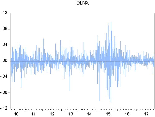
Figure 2. Daily return of CSI 300.

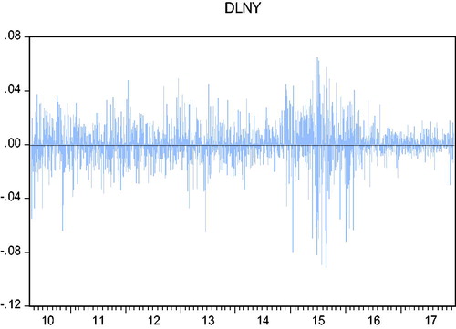
Table 3. ARCH effect test of ${\epsilon }_{st}$ and ${\epsilon }_{ft}$ sequences of ECM model.

${\epsilon }_{st}$
$F$	54.5940	p value.$F$(5, 1851)	0.0000
$T{R}^2$	238.6595	p value.${\chi }^2(5)$	0.0000
${\epsilon }_{ft}$
$F$	93.0210	p value.$F$(5, 1851)	0.0000
$T{R}^2$	372.9107	p value.${\chi }^2(5)$	0.0000

In Table 3, both the statistic $F$ and the statistic $T{R}^2$ significantly reject the null hypothesis, indicating that autoregressive conditional heteroscedasticity exists in the error term, so the ECM-GARCH model can be applied. First, the residual $e_{st}$ and conditional variance ${\sigma }_{ss,t}^2$ can be obtained by estimating the GARCH (1, 1) model for $\Delta \hspace{0.17em}\text{ln}\hspace{0.17em}{S}_t;$ similarly, the residual $e_{ft}$ and conditional variance ${\sigma }_{ff,t}^2$ can be acquired. Through the residuals $e_{st}$ and $e_{ft},$ we find that the correlation coefficient is 0.9285. The conditional covariance ${\sigma }_{sf,t}$ can be obtained from Equation (7)(7) $${\sigma }_{sf,t}={\rho }_{sf}{\sigma }_{ss,t-1}{\sigma }_{ff,t-1}$$(7) . The dynamic optimal hedging ratio $h_{t-1}^{*}$ and the dynamic hedging effectiveness $H_{e,t}^{*}$ can be calculated by Equations (8)(8) $$h_{t-1}^{*}=\frac{\mathit{Cov}(\Delta \hspace{0.17em}\text{ln}\hspace{0.17em}{S}_t,\Delta \hspace{0.17em}\text{ln}\hspace{0.17em}{F}_t|{\psi }_{t-1})}{\mathit{Var}(\Delta \hspace{0.17em}\text{ln}\hspace{0.17em}{F}_t|{\psi }_{t-1})}=\frac{\mathit{Cov}({\epsilon }_{st},{\epsilon }_{ft}|{\psi }_{t-1})}{\mathit{Var}({\epsilon }_{ft}|{\psi }_{t-1})}=\frac{{\sigma }_{sf,t}}{{\sigma }_{ff,t}^2}$$(8) and (9)(9) $$H_{e,t}=\frac{\mathit{Var}(\Delta \hspace{0.17em}\text{ln}\hspace{0.17em}S)-\mathit{Var}(R(h))}{\mathit{Var}(\Delta \hspace{0.17em}\text{ln}\hspace{0.17em}S)}=\frac{2h_{t-1}^{*}{\sigma }_{sf,t}-h_{t-1}^{*}{}^2{\sigma }_{ff,t}^2}{{\sigma }_{ss,t}^2}$$(9) . The relevant statistical results are summarised in Table 4.

Table 4. Dynamic hedging ratio and effectiveness.

	Mean	Median	Maximum	Minimum	Std.Dev	Skewness	Kurtosis
$h_{t-1}^{*}$	0.8702	0.8765	1.1487	0.3409	0.1192	−0.5887	3.6807
$h_{e,t}^{*}$	0.8611	0.9198	0.9781	−0.3091	0.1521	−2.8135	13.0888

In Table 4, the average daily hedging ratio is 0.8702, and the average effective hedging rate reaches 86.11%. The above results indicate that the CSI 300 stock index futures can perform hedging function well and effectively avoid the systematic risk of spot price fluctuations. It is remarkable that the standard deviations of optimal hedge ratio and the corresponding extent of effectiveness are fairly small, strongly indicating that fewer adjustments of the numbers of futures contracts are required with the ECM-GARCH hedging strategy. In other words, fewer transaction costs are required using the ECM-GARCH hedging model and the best hedging and high efficiency can be achieved as long as the operation is appropriate.

5.2. Empirical test of arbitrage

The arbitrage function of stock index futures can be effectively examined by means of the analysis of the cointegration relationship and the error correction model. According to the general idea, we start with the linear vector error correction model. First, we check the cointegration relationship between variables. By using the ADF unit root test, it is found that $\text{ln}\hspace{0.17em}F$ and $\text{ln}\hspace{0.17em}S$ are both integrated of order 1 $I(1);$ therefore, we can continue to conduct the cointegration test. Using the Johansen cointegration test, it is found that there is a cointegration relationship between the sequence $\text{ln}\hspace{0.17em}F$ and $\text{ln}\hspace{0.17em}S.$ The results indicate that there is a stable linear equilibrium relationship between the CSI 300 stock index futures and the spot index throughout the sample period, which implies the short-term price deviation can return to equilibrium through dynamic adjustment. We can make a preliminary inference that the arbitrage function of CSI 300 stock index futures have been played to a certain extent since the short-term arbitrage behaviour in the stock index futures market only has the effect of bridging these price deviations.

To verify the above conjecture, we further establish a VECM model to investigate the short-term error correction mechanism of the system. The estimated results of the linear VECM model are expressed as follows: $$\{\begin{array}{c}\Delta \hspace{0.17em}\text{ln}\hspace{0.17em}{S}_t=0.0001-0.03e_{t-1}-0.29\Delta \hspace{0.17em}\text{ln}\hspace{0.17em}{S}_{t-1}+0.32\Delta \hspace{0.17em}\text{ln}\hspace{0.17em}{F}_{t-1}\\ (0.0004)(0.03)(0.06)(0.05)\\ \Delta \hspace{0.17em}\text{ln}\hspace{0.17em}{F}_t=0.0001+0.13e_{t-1}-0.21\Delta \hspace{0.17em}\text{ln}\hspace{0.17em}{S}_{t-1}+0.20\Delta \hspace{0.17em}\text{ln}\hspace{0.17em}{F}_{t-1}\\ (0.0004)(0.04)(0.07)(0.06)\end{array}$$ where $e_{t-1}=\hspace{0.17em}\text{ln}\hspace{0.17em}{S}_{t-1}-1.01\hspace{0.17em}\text{ln}\hspace{0.17em}{F}_{t-1}+0.10.$ It can be seen that all lag price changes are significant. The error correction coefficient in the stock index futures equation is significant, however, while that in the index equation is reversed. Since the main purpose of this study is to examine the functional efficiency, both the arbitrage function test and the subsequent test of the price discovery function require us to focus on short-term dynamics. For long-term equilibrium, the significance of the linear vector error correction equation of futures implies that there is a cointegration relationship between futures and spots. We suspect that the phenomenon that the error correction mechanism exists only in the stock index futures market may be related to the fact that stock index futures participate in the transaction, while index spots serve as references for market quotations only.

Considering the possible nonlinear characteristics of dynamic adjustment in terms of arbitrage, we further construct a threshold vector error correction model (T-VECM) by referring to the method of Hansen and Seo (2002). The estimated results of the T-VECM model are expressed as follows: $$\Delta \hspace{0.17em}\text{ln}\hspace{0.17em}{S}_t=\{\begin{array}{c}-0.004-0.06w_{t-1}-0.23\Delta \hspace{0.17em}\text{ln}\hspace{0.17em}{S}_{t-1}+0.21\Delta \hspace{0.17em}\text{ln}\hspace{0.17em}{F}_{t-1}+{\mu }_{1t},w_{t-1}\le -0.07\\ (0.006)(0.07)(0.13)(0.12)\\ 0.010+0.21w_{t-1}-0.31\Delta \hspace{0.17em}\text{ln}\hspace{0.17em}{S}_{t-1}+0.47\Delta \hspace{0.17em}\text{ln}\hspace{0.17em}{F}_{t-1}+{\mu }_{1t},w_{t-1}>-0.07\\ (0.01)(0.20)(0.21)(0.15)\end{array}$$ $$\Delta \hspace{0.17em}\text{ln}\hspace{0.17em}{F}_t=\{\begin{array}{c}0.007+0.08w_{t-1}+0.02\Delta \hspace{0.17em}\text{ln}\hspace{0.17em}{S}_{t-1}-0.07\Delta \hspace{0.17em}\text{ln}\hspace{0.17em}{F}_{t-1}+{\mu }_{2t},w_{t-1}\le -0.07\\ (0.007)(0.08)(0.13)(0.13)\\ 0.031+0.52w_{t-1}-0.49\Delta \hspace{0.17em}\text{ln}\hspace{0.17em}{S}_{t-1}+0.63\Delta \hspace{0.17em}\text{ln}\hspace{0.17em}{F}_{t-1}+{\mu }_{2t},w_{t-1}>-0.07\\ (0.01)(0.21)(0.27)(0.19)\end{array}$$ where $w_{t-1}=\hspace{0.17em}\text{ln}\hspace{0.17em}{S}_{t-1}-1.01\hspace{0.17em}\text{ln}\hspace{0.17em}{F}_{t-1}.$ It can be seen that the threshold value −0.07 divides the error correction model into two regimes, where the first regime ($w_{t-1}\le -0.07$) accounts for 94% of the observed value, while the second regime ($w_{t-1}>-0.07$) accounts for only 6% of the observed value. We label the former and the latter as the ‘typical’ regime and ‘extreme’ regime, respectively. In the typical regime, no coefficients of the spots equation or the futures equation are significant. The error correction effect and dynamic coefficient in the typical regime are much smaller than in the extreme regime. According to the understanding of Hansen and Seo (2002), they are closing in to the white noise, which indicates that $\text{ln}\hspace{0.17em}{S}_t$ and $\text{ln}\hspace{0.17em}{F}_t$ are close to the drift-free random walk for most of the time and once again confirms the results of the previous variance ratio test.

As for the extreme regime, the coefficient of the stock index futures equation is significant, except that the coefficient of $\Delta \hspace{0.17em}\text{ln}\hspace{0.17em}{S}_{t-1}$ is at the statistically significant boundary, while the coefficients of the index equation are not significant, except for the coefficient of $\Delta \hspace{0.17em}\text{ln}\hspace{0.17em}{F}_{t-1}.$ This finding is very similar to those obtained with the linear VECM model. As far as the results are concerned, the linear model and the threshold model consistently indicate that the system has a certain error correction mechanism that is maintained by stock index futures. More importantly, there is an obvious threshold effect in the error correction mechanism, which indicates that there is little arbitrage opportunity for stock index futures (6%).

5.3. Empirical test of price discovery

The price discovery function of the stock index futures market is mainly reflected in the fact that stock index futures can reflect the information shocks more quickly and adjust the price more rapidly, resulting in the price change running ahead of that in index spots. Since the Granger causality test can test whether the short-term lag of one variable has a ‘predictive’ ability for another variable, it can test the short-term lead-lag relationship between stock index futures and index spots.

Because there is at least one unidirectional Granger causality between cointegration variables, linear Granger causality tests can be performed on cointegration variables $\text{ln}\hspace{0.17em}S$ and $\text{ln}\hspace{0.17em}F.$ Consider the possible nonlinear characteristics in price discovery, we apply both linear and nonlinear Granger causality tests to the whole sample and each subsample. The linear Granger causality test is based on the optimal VAR model determined by the AIC information criterion. The nonlinear Granger causality test proposed by Diks and Panchenko (2006) is conducted by running a $T_n$ test on the residual of the above optimal VAR model. Table 5 summarises the linear and nonlinear Granger test results.

Table 5. Results of linear and nonlinear Granger test.

$l_S=l_F$	$\text{ln}\hspace{0.17em}S\Rightarrow \hspace{0.17em}\text{ln}\hspace{0.17em}F$		$\text{ln}\hspace{0.17em}F\Rightarrow \hspace{0.17em}\text{ln}\hspace{0.17em}S$
	$F$	$T_2$	$F$		$T_2$
Whole sample (4/16/2010–12/13/2017, 1864 obs.）
1	7.407***	1.546*		7.132***		3.530***
2	8.397***	2.572***		20.32***		2.913***
3	6.136***	2.169**		13.44***		2.121**
4	13.11***	2.738***		10.68***		0.937
5	9.615***	3.065***		8.117***		1.450*
6	7.950***	3.026***		6.754***		0.897
7	7.440***	2.930***		6.300***		0.863
8	6.851***	2.992***		6.130***		0.995
Group A: (4/16/2010–6/10/2011, 279 obs.）
1	6.364**	−0.828		0.345		1.362*
2	2.561*	−1.623		1.531		0.667
3	1.745	−0.833		1.093		1.657**
4	2.501**	−0.774		1.589		1.343*
5	2.327**	−0.756		1.551		1.274
Group B (6/13/2011–1/29/2013, 400 obs.)
1	2.019	−1.795		3.235*		0.698
2	1.07	−1.333		1.542		0.68
3	0.68	−2.054		0.995		−0.701
4	0.513	−1.784		0.838		−0.537
5	1.43	−2.09		1.664		−0.971
Group C (1/30/2013–3/11/2015,508 obs.)
1	1.44	0.249		3.596*		2.384***
2	1.684	1.25		4.304**		2.392***
3	1.205	1.211		3.160**		1.985**
4	0.919	1.056		2.441**		1.970**
5	1.344	1.171		2.075*		1.976**
GroupD (3/12/2015–4/28/2016,279 obs.)
1	0.24	1.002		6.818***		1.494*
2	2.186	1.461*		6.243***		1.410*
3	1.338	0.807		5.021***		0.792
4	3.488***	0.549		4.217***		0.847
5	2.060*	0.931		2.878**		0.399
Group E (4/29/2016–12/13/2017,398 obs.)
1	8.828***	1.985**		0.398		−2.135
2	4.497**	0.7		0.357		−2.74
3	3.291**	−0.313		0.466		−1.594
4	3.490***	−0.224		1.186		−1.324
5	2.018*	−0.213		0.985		0.873

In Table 5, statistic $F$ and statistic $T_2$ represent linear and nonlinear Granger causality tests, respectively. $l_S=l_Y$ shows the common lag order that represents the lag period of the logarithmic price in the linear causality test and the residual lag order of the optimal VAR model in the nonlinear causality test. The statistic $T_2$ is given by Equation (11)(11) $$\frac{f_{X,Y,Z}(x,y,z)}{f_Y(y)}=\frac{f_{X,Y}(x,y)}{f_Y(y)}\frac{f_{Y,Z}(y,z)}{f_Y(y)}$$(11) , and the bandwidth is determined by Equation (12)(12) $$\frac{C_{X,Y,Z}(\epsilon )}{C_Y(\epsilon )}=\frac{C_{X,Y}(\epsilon )}{C_Y(\epsilon )}\frac{C_{Y,Z}(\epsilon )}{C_Y(\epsilon )}$$(12) . After calculation, except for the bandwidth of the whole sample selected as 1.0, the bandwidth of each subsample is 1.5.

By using the whole sample, the$F$ tests how significant bidirectional linear Granger causality. Moreover, the leadership can be observed with more lagged periods, which indicates that index futures and index spots both have a strong linear leading effect in the long run. For each subsample, we analyse from the horizontal and vertical angles. From the horizontal perspective, the index spots in Group A show a more significant linear leading function, while the stock index futures show a certain nonlinear leading effect. Neither the index spots nor the stock index futures in Group B show significant linear or nonlinear leadership. In Groups C and D, the stock index futures show a significant linear and nonlinear leading effect, while the index spots show the opposite. The nonlinear leading effect weakens with the increasing of the linear leading effect. In Group E, the index spots show a significant linear leader ship again with a weak nonlinear leading effect. From the vertical perspective, there is a linear guiding effect of the index spots, index futures, index futures and index spots, in turn, since the listing of CSI 300 index futures, interspersed with a period of no leading effect. In addition, it is worth noting that nonlinear leadership is mainly reflected in stock index futures, which is in line with our expectations for index futures.

The above results reveal that the lead-lag relationship between index futures and index spots is time-varying. Due to the incomparable advantages of futures markets, such as inherent leverage, low transaction costs, and the absence of any short-selling constraints, it is widely accepted that futures markets are supposed to incorporate information more efficiently than spot markets. The results of subsample A, B and E, however, run counter to this expectation. We can speculate about possible causes of this time-varying phenomenon in the light of existing research. For subsample A, we assume that the phenomenon that index spots guide index futures may be closely related to the fact that stock index futures have just been listed. For subsample B, the index spot leadership disappears and there is no lead-lag relationship in each market, which may be due to the withdrawal of the bear market and mean that the price guidance relationship is undergoing adjustment. Chatrath, Christie‐David, Dhanda, and Koch (2002) show evidence of pronounced futures leadership when markets are rising. When markets are falling, futures leadership is less obvious and significant feedback from the cash market is observed. In subsamples C and D, index futures a show good price discovery function, while there is little evidence supporting that the index spot has pronounced leadership. In subsample E, however, the role of leadership reversed unexpectedly once again. Lien et al. (2003) report that the spot market leads the futures market when structural change occurs in the spot index, and the spot market is more informationally efficient than the futures market under high variance conditions in Li (2009). We infer that this reversal may be influenced by a series of institutional changes and major financial events in the first half of 2016, such as the fuse mechanism (including implementation and suspension), new rules for reducing shareholdings (for major shareholders and directors), the depreciation of the RMB and the implementation of the registration system.

6. Conclusions

In this study, we first establish an empirical framework to test the efficiency of the CSI 300 index futures markets from the perspective of information efficiency and function efficiency, and then examine the nonlinear dynamic characteristics of the efficiency of the CSI 300 index futures market by using nonparametric methods.

In terms of information efficiency, we find that the prices of stock index futures follow a random walk or a martingale process throughout the whole sample period or in each subsample interval. According to the effective market hypothesis (Malkiel & Fama, 1970), there is reason to believe that the CSI 300 stock index futures market has reached a weak form of informational effectiveness in both the long term and the short term. The results indicate that the current stock index futures contract price has reflected all historical trading information in the market, and it is impossible for investors to predict price trends and obtain excess profits by analysing historical prices.

Because the CSI 300 stock index futures market has achieved weak information effectiveness, we can continue to examine the functional efficiency. For hedging, the result of the ECM-BGARCH model show that the dynamic optimal hedge ratio has an average of 0.8702 and an average effective level reach of 86.11%, which means that the risk (variance) of the portfolio in the spot market can be reduced by an average of 86.11% after hedging in the CSI 300 stock index futures market. The result is basically in line with findings from some previous studies (Hou & Li, 2013; Yan & Li, 2018), and confirms that the CSI 300 stock index futures market can avoid the systemic risk of the stock index market. This result also shows that the potential optimal hedging can be achieved as long as we accurately grasp the real price linkages between futures and spots.

Regarding arbitrage, the results show that the error correction mechanism is supported only by stock index futures. Additionally, the error correction effect only exists in the extreme regime (only 6% of the total observed value), which means that arbitrage opportunities are rare and arbitrage trades account for only 6% of the total observed value. Most of the time (94% of all observations), both prices are subject to the random walk process and there is no arbitrage trade between futures and spots. This result shows that stock index futures pricing is reasonable without too many arbitrage opportunities and can exert the function of arbitrage normally to screen the unreasonable fluctuation of the stock market when there are arbitrage opportunities. In terms of price discovery, the empirical results show that in stock index futures, there is both linear leadership and nonlinear leadership that was not recognised by the Granger causality test. The nonlinear leadership was mainly reflected in stock index futures. Neither linear nor nonlinear leadership, however, are as stable as we expected. The results of the subsamples divided by breakpoints show that both linear and nonlinear leadership exist in one period and disappear in another period. Influenced by institutional changes and significant financial events, index futures cannot play a steady dominant role in price discovery, which indicates that the price discovery function of stock index futures must be further improved.

In sum, we can conclude that the CSI 300 stock index futures market is basically effective despite the flaws in price discovery. On the basis of weak information effectiveness, CSI 300 stock index futures have performed the function of hedging and arbitrage well to avoid the systematic risks of spot price fluctuations and screened the unreasonable fluctuations of the stock market. Influenced by financial events and mechanism changes; however, the stock index futures cannot exert price discovery function stably.

In our study, the results of information efficiency and hedging functions are basically consistent with previous studies of financial markets in developed countries (Dark, 2015; Evans, 2006; Markopoulou et al., 2016.) We also find new results for arbitrage showing that the short-term dynamic adjustment process happens only when the difference between the index futures price and index spots price exceeds the threshold, despite the existence of a long-term cointegration relationship. This nonlinear error correction mechanism reflected in the outside minor arbitrage trades actually guarantees the long-term equilibrium relationship over the entire sample period. For price discovery, ignored by most previous studies, we find that there is not only linear leadership but also nonlinear leadership in CSI 300 stock index futures. The nonlinear leadership was mainly reflected in stock index futures. More importantly, influenced by institutional changes and significant financial events, both the linear and nonlinear leadership of stock index futures evolved over the sample period.

This study has some limitations. First, comparing the daily data we used in this study, higher frequency intraday data is able to capture more details of dynamics between index futures and spots than daily data. Second, the effect of hedging may be further improved by combining ECM-BGARCH with the prevailing Markov switching (MS), long memory and asymmetries in volatility, which is worth future examination. Finally, it will be interesting to explore the determinants of the effective stock index futures market and the reasons for instability in the price discovery function. The above limitations will be the main direction for further research.

Disclosure statement

No potential conflict of interest was reported by the authors.

Additional information

Funding

We gratefully acknowledge the support of Chinese Ministry of Education Humanities and Social Science Youth Fund under Grant 19YJC790105.

References

- Al‐Khazali, O. M., Ding, D. K., & Pyun, C. S. (2007). A new variance ratio test of random walk in emerging markets: A revisit. The Financial Review, 42(2), 303–317. doi:10.1111/j.1540-6288.2007.00173.x
- Baek, E. G., & Brock, W. A. (1992). A nonparametric test for independence of a multivariate time series. Statistica Sinica, 2(1), 137–156. doi:10.5705/ss.202018.0159
- Belaire-Franch, J., & Contreras, D. (2004). Ranks and signs-based multiple variance ratio tests. Working paper. https://www.researchgate.net/publication/228583649_Ranks_and_signs-based_multiple_variance_ratio_tests.
- Białkowski, J., & Jakubowski, J. (2008). Stock index futures arbitrage in emerging markets: Polish evidence. International Review of Financial Analysis, 17(2), 363–381. doi:10.1016/j.irfa.2006.10.004
- Bollerslev, T. (1990). Modelling the coherence in short-run nominal exchange rates: A multivariate generalized ARCH model. The Review of Economics and Statistics, 72(3), 498–505. doi:10.2307/2109358
- Brennan, M. J., & Schwartz, E. S. (1990). Arbitrage in stock index futures. The Journal of Business, 63(S1), S7–S31. doi:10.1086/296491
- Camelia, O., Cristina, T., & Amelia, B. (2017). A new proposal for efficiency quantification of capital markets in the context of complex non-linear dynamics and chaos. Economic Research-Ekonomska Istraživanja, 30(1), 1669–1692. doi:10.1080/1331677X.2017.1383172
- Campbell, B., & Dufour, J. M. (1997). Exact nonparametric tests of orthogonality and random walk in the presence of a drift parameter. International Economic Review, 38(1), 151–173. doi:10.2307/2527412
- Chatrath, A., Christie‐David, R., Dhanda, K. K., & Koch, T. W. (2002). Index futures leadership, basis behavior, and trader selectivity. Journal of Futures Markets, 22(7), 649–677. doi:10.1002/fut.10026
- Chen, Y. L., & Gau, Y. F. (2009). Tick sizes and relative rates of price discovery in stock, futures, and options markets: Evidence from the Taiwan stock exchange. Journal of Futures Markets, 29(1), 74–93. doi:10.1002/fut.20319
- Chen, Y. L., & Tsai, W. C. (2017). Determinants of price discovery in the VIX futures market. Journal of Empirical Finance, 43, 59–73. doi:10.1016/j.jempfin.2017.05.002
- Chow, K. V., & Denning, K. C. (1993). A simple multiple variance ratio test. Journal of Econometrics, 58(3), 385–401. doi:10.1016/0304-4076(93)90051-6
- Cornell, B., & French, K. R. (1983). The pricing of stock index futures. Journal of Futures Markets, 3(1), 1–14. doi:10.1002/fut.3990030102
- Creamer, G. G., & Creamer, B. (2016). A nonlinear lead lag dependence analysis of energy futures: Oil, coal, and natural gas. In I. Florescu, M. C. Mariani, H. E. Stanley, & F. G. Viens (Eds.), Handbook of high-frequency trading and modeling in finance (Vol. 9, pp. 61–71). New Jersey, United States: John Wiley & Sons Inc.
- Dark, J. (2015). Futures hedging with Markov switching vector error correction FIEGARCH and FIAPARCH. Journal of Banking & Finance, 61, S269–S285. doi:10.1016/j.jbankfin.2015.08.017
- Davies, R. B. (1987). Hypothesis testing when a nuisance parameter is present only under the alternative. Biometrika, 74(1), 33–43. doi:10.1093/biomet/74.1.33
- Diks, C., & Panchenko, V. (2006). A new statistic and practical guidelines for nonparametric Granger causality testing. Journal of Economic Dynamics and Control, 30(9-10), 1647–1669. doi:10.1016/j.jedc.2005.08.008
- Ederington, L. H. (1979). The hedging performance of the new futures markets. The Journal of Finance, 34(1), 157–170. doi:10.1111/j.1540-6261.1979.tb02077.x
- Engle, R. (2002). Dynamic conditional correlation: A simple class of multivariate generalized autoregressive conditional heteroskedasticity models. Journal of Business & Economic Statistics, 20(3), 339–350. doi:10.1198/073500102288618487
- Engle, R. F., & Kroner, K. F. (1995). Multivariate simultaneous generalized ARCH. Econometric Theory, 11(1), 122–150. doi:10.1017/S0266466600009063
- Evans, T. (2006). Efficiency tests of the UK financial futures markets and the impact of electronic trading systems. Applied Financial Economics, 16(17), 1273–1283. doi:10.1080/09603100500438767
- Forbes, C. S., Kalb, G. R., & Kofhian, P. (1999). Bayesian arbitrage threshold analysis. Journal of Business & Economic Statistics, 17(3), 364–372. doi:10.1080/07350015.1999.10524825
- Frijns, B., & Zwinkels, R. C. (2018). Time-varying arbitrage and dynamic price discovery. Journal of Economic Dynamics and Control, 91, 485–502. doi:10.1016/j.jedc.2018.03.014
- Hansen, B. E., & Seo, B. (2002). Testing for two-regime threshold cointegration in vector error-correction models. Journal of Econometrics, 110(2), 293–318. doi:10.1016/S0304-4076(02)00097-0
- Hiemstra, C., & Jones, J. D. (1994). Testing for linear and nonlinear Granger causality in the stock price‐volume relation. The Journal of Finance, 49(5), 1639–1664. doi:10.2307/2329266
- Hou, Y., & Li, S. (2013). Hedging performance of Chinese stock index futures: An empirical analysis using wavelet analysis and flexible bivariate GARCH approaches. Pacific-Basin Finance Journal, 24, 109–131. doi:10.1016/j.pacfin.2013.04.001
- Hou, Y., & Li, S. (2015). Volatility behaviour of stock index futures in China: A bivariate GARCH approach. Studies in Economics and Finance, 32(1), 128–154.
- Huang, B. N. (1995). Do Asian stock market prices follow random walks? Evidence from the variance ratio test. Applied Financial Economics, 5(4), 251–256. doi:10.1080/758536875
- Huang, B. N., Yang, C. W., & Hwang, M. J. (2009). The dynamics of a nonlinear relationship between crude oil spot and futures prices: A multivariate threshold regression approach. Energy Economics, 31(1), 91–98. doi:10.1016/j.eneco.2008.08.002
- Judge, A., & Reancharoen, T. (2014). An empirical examination of the lead–lag relationship between spot and futures markets: Evidence from Thailand. Pacific-Basin Finance Journal, 29, 335–358. doi:10.1016/j.pacfin.2014.05.003
- Kim, B. H., Chun, S. E., & Min, H. G. (2010). Nonlinear dynamics in arbitrage of the S&P 500 index and futures: A threshold error-correction model. Economic Modelling, 27(2), 566–573.
- Kim, J. H. (2009). Automatic variance ratio test under conditional heteroskedasticity. Finance Research Letters, 6(3), 179–185. doi:10.1016/j.frl.2009.04.003
- Kroner, K. F., & Sultan, J. (1993). Time-varying distributions and dynamic hedging with foreign currency futures. The Journal of Financial and Quantitative Analysis, 28(4), 535–551. doi:10.2307/2331164
- Lai, Y. S. (2019). Evaluating the hedging performance of multivariate GARCH models. Asia Pacific Management Review, 24(1), 86–95. doi:10.1016/j.apmrv.2018.07.003
- Lee, H. T. (2009). Optimal futures hedging under jump switching dynamics. Journal of Empirical Finance, 16(3), 446–456. doi:10.1016/j.jempfin.2008.12.001
- Lee, H. T., & Yoder, J. K. (2007). A bivariate Markov regime switching GARCH approach to estimate time varying minimum variance hedge ratios. Applied Economics, 39(10), 1253–1265. doi:10.1080/00036840500438970
- Li, M. Y. L. (2009). The dynamics of the relationship between spot and futures markets under high and low variance regimes. Applied Stochastic Models in Business and Industry, 25(6), 696–718. doi:10.1002/asmb.753
- Lien, D. H. D. (1996). The effect of the cointegration relationship on futures hedging: A note. Journal of Futures Markets, 16(7), 773–780. doi:10.1002/(SICI)1096-9934(199610)16:7<773::AID-FUT3>3.0.CO;2-L
- Lien, D., Tse, Y. K., & Zhang, X. (2003). Structural change and lead-lag relationship between the Nikkei spot index and futures price: A genetic programming approach. Quantitative Finance, 3(2), 136–144. doi:10.1088/1469-7688/3/2/307
- Lo, A. W., & MacKinlay, A. C. (1989). The size and power of the variance ratio test in finite samples: A Monte Carlo investigation. Journal of Econometrics, 40(2), 203–238.
- Lo, M. C., & Zivot, E. (2001). Threshold cointegration and nonlinear adjustment to the law of one price. Macroeconomic Dynamics, 5(4), 533–576. doi:10.1017/S1365100501023057
- Luger, R. (2003). Exact non-parametric tests for a random walk with unknown drift under conditional heteroscedasticity. Journal of Econometrics, 115(2), 259–276. doi:10.1016/S0304-4076(03)00097-6
- Malkiel, B. G., & Fama, E. F. (1970). Efficient capital markets: A review of theory and empirical work. The Journal of Finance, 25(2), 383–417. doi:10.1111/j.1540-6261.1970.tb00518.x
- Markopoulou, C. E., Skintzi, V. D., & Refenes, A. P. N. (2016). Realized hedge ratio: Predictability and hedging performance. International Review of Financial Analysis, 45, 121–133. doi:10.1016/j.irfa.2016.03.005
- Martinez, V., & Tse, Y. (2018). Intraday price discovery analysis in the foreign exchange market of an emerging economy: Mexico. Research in International Business and Finance, 45, 271–284. doi:10.1016/j.ribaf.2017.07.159
- Miao, H., Ramchander, S., Wang, T., & Yang, D. (2017). Role of index futures on China’s stock markets: Evidence from price discovery and volatility spillover. Pacific-Basin Finance Journal, 44, 13–26. doi:10.1016/j.pacfin.2017.05.003
- Okur, M., & Cevik, E. (2013). Testing intraday volatility spillovers in Turkish capital markets: Evidence from ISE. Economic research-Ekonomska Istraživanja, 26(3), 99–116. doi:10.1080/1331677X.2013.11517624
- Patton, A. J. (2009). Copula–based models for financial time series. In T. Mikosch, J.-P. Kreiß, R. A. Davis, & T. G. Andersen (Eds.), Handbook of financial time series (pp. 767–785). Berlin: Springer.
- Qu, H., Wang, T., Zhang, Y., & Sun, P. (2018). Dynamic hedging using the realized minimum-variance hedge ratio approach–Examination of the CSI 300 index futures. Pacific-Basin Finance Journal, 101048. doi:10.1016/j.pacfin.2018.08.002
- Samuelson, P. A. (2016). Proof that properly anticipated prices fluctuate randomly. In G. M. Anastasios, & T. Z. William (Eds.), The world scientific handbook of futures markets (pp. 25–38). Singapore: World Scientific.
- Silvapulle, P., & Moosa, I. A. (1999). The relationship between spot and futures prices: Evidence from the crude oil market. Journal of Futures Markets, 19(2), 175–193. doi:10.1002/(SICI)1096-9934(199904)19:2<175::AID-FUT3>3.3.CO;2-8
- Tse, Y. K., & Chan, W. S. (2010). The lead–lag relation between the S&P500 spot and futures markets: An intraday-data analysis using a threshold regression model. The Japanese Economic Review, 61(1), 133–144.
- Wright, J. H. (2000). Alternative variance-ratio tests using ranks and signs. Journal of Business & Economic Statistics, 18(1), 1–9. doi:10.2307/1392131
- Yan, Z. P., & Li, S. H. (2018). Hedge ratio on Markov regime-switching diagonal Bekk–Garch model. Finance Research Letters, 24, 49–55.
- Yang, J., & Awokuse, T. O. (2003). Asset storability and hedging effectiveness in commodity futures markets. Applied Economics Letters, 10(8), 487–491. doi:10.1080/1350485032000095366
- Yang, J., Yang, Z., & Zhou, Y. (2012). Intraday price discovery and volatility transmission in stock index and stock index futures markets: Evidence from China. Journal of Futures Markets, 32(2), 99–121. doi:10.1002/fut.20514
- Yi, Q., & Liang, Z. (2014). The information efficiency of stock index futures in China. In J. Xu, J. A. Fry, B. Lev, & A. Hajiyev (Eds.), Proceedings of the seventh international conference on management science and engineering management (pp. 1041–1050). Berlin: Springer.