A multivariate cointegration time series model and its applications in analysing stock markets in China

Abstract

This paper explores nonlinear cointegration between Chinese mainland stock markets and Hong Kong stock market in a multivariate framework for the period January, 1998 to December, 2014 by a nonparametric method. The local linear kernel smoothing method is developed to estimate the unknown function, and the practical problem of implementation is also addressed. Then, a simple nonparametric version of a bootstrap test is adapted for testing misspecification. Furthermore, Some Monte Carlo experiments are presented to examine the finite sample performance of the proposed procedure. Finally, the stock markets data set is discussed in detail by using proposed procedures, showing that Shanghai Stock Index (SHSI) and Shenzhen Component Index (SZCI) can affect Hang Seng Index (HSI), and the influence appears to be a strong nonlinear characteristics.

Keywords:

• Local linear estimation
• misspecification test
• multivariate nonlinear cointegration
• time series

JEL CLASSIFICATIONS:

• C14
• C22
• G15

1. Introduction

China is one of the fastest-growing economies in the world. According to International Monetary Fund (IMF) and purchasing power parity (PPP), Chinese economy is the second largest in the world by nominal GDP. China’s financial sector, especially stock market has complemented the growth process significantly since the onset of financial reforms in the late nineties. Over the past two decades, the stock market has grown stupendously in terms of increase in size and volume of investment by both domestic and international investors. The relationship between stock prices and macroeconomic variables has been discussed all over the world. The growing linkages between macroeconomic variables and the movement of stock prices have well been documented in the literature over the last several years (Sadorsky, 2003; Chen, 2003; Hadi, Katircioğlu, & Adaoglu, 2019; Katircioğlu, Alkhazaleh, & Katircioğlu, 2018; Katircioğlu & Zabolotnov, 2019; Rezgallah, Özataç, & Katircioğlu, 2019; Shaeri & Katircioğlu, 2018). Campbell (1987, 1991), Fama and Schwert (1997) showed that short- and long-term interest rates have a modest degree of forecasting power for excess stock returns. Similarly, other studies, such as Campbell and Shiller (1991) and Fama (1984), have shown that the slope of the term structure of interest rates helps to forecast excess stock returns. On the other hand, Campbell and Ammer (1993) showed that short-term interest rates affect stock prices. Daily stock prices are determined by many factors, including enterprise performance, dividends, other countries stock prices, gross domestic product, exchange rates, interest rates, current account, money supply, employment, and so on. Countless factors impact stock prices. In China, the regional stock exchanges from Shanghai, Shenzhen and Hong Kong simultaneously reflect the country’s economy. For the different locations, economic development backgrounds and trading rules, the three stock markets are showing different operating characteristics. To better explore the susceptibility the movements of of stock market in relation to country’s macroeconomic indicators and fashion investment decisions and policy decisions for investors and policy makers, it is necessary to study the contact of the three stock markets.

The study of linear nonstationary time series and linear cointegration relationships has led to a huge development in macro econometrics and financial econometrics, since most of macro and financial time series exhibit nonstationary features. One of the main disadvantages of conventional linear cointegration methodologies is that it assumes that the cointegrating relationship does not change over the entire data span, which is too unrealistic to be true especially when the time series is long, such as Johansen (1988, 1991, 1995), Johansen and Juselius (1990), Pesaran and Shin (1998), and Pesaran, Shin, and Smith (2001) for more details. Recently, there is a growing interest on the nonlinear properties of nonstationary time series. In this article, we investigate the local linear estimation of a nonparametric multivariate cointegration model of the form (1) $$Y_t=f(X_t)+u_t,\hspace{1em}t=1,\dots ,n,$$(1) where X_t is d-dimensional predictor variable with each element I(1) process, $f(·)$ is an unknown to be estimated with the observed data ${\{X_t,Y_t\}}_{t=1}^n$ but sufficiently smooth function, and u_t is an I(0) process.

When X_t is a univariate I(1) process, model (1) has been studied by many researchers. For instance, Kanas (2003) used the alternating conditional expectations (ACE) algorithm to nonlinearly transform stock prices and dividends for the USA for the period 1871–1999 and found strong evidence of cointegration between the transformed variables, which could be characterized as nonlinear cointegration. Karlsen, Myklebust, and Tjøstheim (2007) discussed the estimation of model (1) by the local constant kernel estimator and derive the asymptotic result under the framework of null recurrent Markov chains which include the unit root process as a special case. Based on the local constant kernel estimator, Wang and Phillips (2009a) developed the asymptotic theory for local time density estimation for a general class of functionals of integrated and fractionally integrated time series. Wang and Phillips (2009b) investigated model (1) with endogeneity, i.e., there is dependence between the nonstationary regressor X_t and the stationary error u_t. They show that the local constant kernel estimator is consistent and the limit distribution is mixed normal. Furthermore, by using local linear method, Liang, Lin, and Hsiao (2015) studied model (1), and derived the properties of the local linear estimator in the nonstationary setting. They also considered a data-driven method to select the bandwidth, and found a drastic improvement of the mean squared errors of the local linear estimator compared to the local constant estimator. Other papers include Breitung (2002); Ma and Kanas (2004); Bae, Kakkar, and Ogaki (2006); Jawadi, Bruneau, and Sghaier (2009); Cross and Worden (2011); and Ghosh and Kanjilal (2014) and reference therein. To our best known, however, a study on the estimation and application of multivariate nonlinear cointegration has been missing.

The development of the multivariate cointegration time series models was motivated by structural modeling of stock markets data of stock data of China. The data set consisting of 204 observations from Shanghai Stock Market, Shenzhen Stock Market and Hong Kong Stock Market, respectively, which can be obtained from http://finance.sina.com.cn/. The data is from January, 1998 to December, 2014 and the monthly closing prices of three market indexes are used. The interest of our study is to analyze the long-term relationship among SHSI ($\left\{P_{1t}\right\}$), SZCI ($\left\{P_{2t}\right\}$) and HSI ($\left\{P_{3t}\right\}$). Some financial time series such as quarterly earning per share of a company exhibits certain seasonality. In some applications, seasonality is of secondary importance and is removed from the data, resulting in a seasonally adjusted time series that is then used to make inference. Detailed analysis of the data set is reported in Section 4.

It is well known that in the stationary setup the local linear kernel estimator is superior to the local constant kernel estimator because it has less finite sample bias and no boundary effect, see Fan and Gijbels (1996). Therefore, in this article, we extend the local linear estimator to deal with the estimation of multivariate cointegration models. Also, we consider a data-driven method to select the bandwidth matrix. Further, the proposed method is applied to investigate the relationship among three stock markets in China, which shows that the proposed method is valid and accurate.

The plan of the article is as follows. Section 2 gives the selection and pre-processing of data. Section 3 discusses the analysis of stock index and the Granger causality test. Section 4 develops the proposed estimation method and presents an empirical application to stock index data. Section 5 contains the conclusion and discussion.

2. Methodologies and practical issues in model building

This section consists of two parts. In Section 2.1, the proposed local linear estimation is described. Some practical issues in model building are discussed in Section 2.2.

2.1. Local linear estimation

We consider the nonparametric cointegration model (1), where $f(·)$ is a smooth function without other restrictions on its specific functional form. X_t follows an I(1) process, i.e., $X_t=X_{t-1}+{\epsilon }_t,t=1,\dots ,n,$ with $X_0=0$ and ${\epsilon }_t$ being a weakly dependent stationary process. The disturbance u_t is a stationary process, i.e., an I(0) process.

For nonparametric regression models with independent and weakly dependent stationary data, it is well established that the local linear estimation method enjoys some optimality properties such as boundary estimation accuracy and minimax efficiency. In this paper, we develop a class of kernel-type nonparametric regression estimators based on local least squares fitting using kernel weights. Much of our attention will be devoted to the local linear least squares kernel estimator of f and its derivative function $f\prime$ which is $\widehat{\alpha }$ and $\widehat{\beta },$ respectively, the solution for α and β to the following problem: (2) $$\text{Minimize}\sum _{t=1}^n{\left\{Y_t-\alpha -{\beta }^{\top }(X_t-x)\right\}}^2{K}_H(X_t-x),$$(2) where x is a given point in a neighborhood of X_t, and H is a d × d symmetric positive definite matrix depending on n, and $K(·)$ is d-variate kernel such that $\int K(u)du=1$ and $K_H(u)=|H{|}^{-1/2}K(H^{-1/2}u).$ We call $H^{1/2}$ the bandwidth matrix since it is the multivariate extension of the usual bandwidth parameter. Problem (2) is a straightforward weighted least squares problem, and assuming that $X^{\top }WX$ is nonsingular, (2) has solution (3) $$\left[\begin{array}{c}\widehat{f}(x)\\ {\widehat{D}}_f(x)\end{array}\right]\equiv \left[\begin{array}{c}\widehat{\alpha }\\ \widehat{\beta }\end{array}\right]={(X^{\top }WX)}^{-1}{X}^{\top }WY,$$(3) where $X=\left[\begin{array}{cc}1& {(X_1-x)}^{\top }\\ ⋮& ⋮\\ 1& {(X_n-x)}^{\top }\end{array}\right],$ $Y={(Y_1,\dots ,Y_n)}^{\top },W=\text{diag}\{K_H(X_1-x),\dots ,K_H(X_n-x)\},$ and $D_f(x)$ denotes the $d\times 1$ vector of first-order partial derivatives. Then, the least squares estimator of $f(·)$ is given by (4) $$\widehat{f}(x;H)=e_1^{\top }{(X^{\top }WX)}^{-1}{X}^{\top }WY,$$(4) where e₁ is the $(d+1)\times 1$ vector having 1 in the first entry and all other entries 0.

It is well known that the bandwidth plays an essential role in the trade-off between reducing bias and variance. Similar to Cai and Tiwari (2000) and Cai (2007), we suggest a nonparametric version of Akaike Information Criterion (AIC) to select the bandwidth matrices. The basic idea is described as follows. For the observed values ${\left\{Y_t\right\}}_{t=1}^n,$ the fitted values $\left\{{\widehat{Y}}_t\right\}$ can be expressed as $\widehat{Y}=S_{H}Y,$ where S_H is a smoother (or hat) matrix associated with the smoothing parameter matrix H. By recalling the AIC for linear models under the likelihood setting $$-2(\text{maximized}\hspace{0.17em}\text{log}\hspace{0.17em}\text{likelihood})+2(\text{number}\text{of}\text{estimated}\text{parameters}),$$

we select the optimal bandwidth matrix H_opt by minimizing $$\text{AIC}(H)=\hspace{0.17em}\text{log}\hspace{0.17em}({\widehat{\sigma }}^2)+\frac{2\left\{\text{tr}(S_H)+1\right\}}{n-\text{tr}(S_H)-2},$$ where ${\widehat{\sigma }}^2$ is an estimate of ${\sigma }^2$ and $\text{tr}(S_H)$ is the trace of S_H, regarded as the nonparametric version degrees of freedom. This selection criterion counteracts the over/under-fitting tendency of the generalized cross-validation and the AIC; see Cai and Tiwari (2000) and Cai (2002) for more details. Alternatively, one might use other existing methods although they may be required more computing; see Yao and Tong (1994), Fan and Gijbels (1996), and Tschernig and Yang (2000).

In practice, it is desirable to have a quick and easy implementation to estimate the asymptotic variance of $\widehat{f}(x)$ to construct a pointwise confidence interval. Specially, we first compute the residuals ${\widehat{u}}_t,$ using the local linear estimation, and then apply a simple moment estimation to obtain a direct and naive estimator of ${\sigma }^2,$ that is, $${\widehat{\sigma }}^2=\frac{1}{n}\sum _{t=1}^n{\widehat{u}}_t^2.$$

It might be shown that ${\widehat{\sigma }}^2$ is a consistent estimate of ${\sigma }^2.$ Therefore, $\widehat{\Sigma }={\widehat{\sigma }}^2{\widehat{\nu }}_0(K)$ is a consistent estimate of Σ, where ${\widehat{\nu }}_0(K)$ is a consistent estimator of ${\nu }_0(K)$ with ${\nu }_0(K)=\int K^2(u)du.$ Other alternative methods might also be applicable here.

2.2. Testing misspecification

In applications, it might be important and interesting to test whether model (1) holds with a specified parametric form. Inspired by Fan, Zhang, and Zhang (2001) and Juhl (2005), we consider the following testing problem (5) $${\mathbf{H}}_0:f(X_t)=g(X_t,\theta ),$$(5) where $g(X_t,\theta )$ is a given function indexed by an unknown parameter vector θ.

For an easy implementation purpose, we adapt a misspecification test by comparing the residual sum of squares (RSS) from both parametric and nonparametric fittings. The testing procedure is described as follows. Let $\widehat{\theta }$ be an estimator of θ. Then, the RSS under ${\mathbf{H}}_0$ is ${\text{RSS}}_0=n^{-1}{\sum }_{t=1}^n{\widehat{u}}_{t,0}^2,$ where ${\widehat{u}}_{t,0}=Y_t-g(X_t,\widehat{\theta })$ and the RSS under ${\mathbf{H}}_a$ is ${\text{RSS}}_1=n^{-1}{\sum }_{t=1}^n{\widehat{u}}_{t,1}^2,$ where ${\widehat{u}}_{t,1}=Y_t-\widehat{f}(X_t).$ Further, the test statistic is defined as $$T_n=\frac{{\text{RSS}}_0-{\text{RSS}}_1}{{\text{RSS}}_1}=\frac{{\text{RSS}}_0}{{\text{RSS}}_1}-1.$$

The null hypothesis (5) is rejected for a large value of T_n. For the sake of simplicity, we evaluate the p-value by using the following nonparametric bootstrap approach, which can be described as follow.

Step 1. Obtain the residuals ${\widehat{u}}_{t,1}=Y_t-\widehat{f}(X_t),$ where $\widehat{f}(·)$ is the local linear estimate of $f(·).$

Step 2. Obtain the bootstrap residuals ${\left\{u_t^{\ast }\right\}}_{t=1}^n$ by randomly resampling with replacement from the set ${\{{\widehat{u}}_{t,1}-{\overline{\widehat{u}}}_{t,1}\}}_{t=1}^n$ with ${\overline{\widehat{u}}}_{t,1}=n^{-1}{\sum }_{t=1}^n{\widehat{u}}_{t,1}.$ Then, $Y_t^{\ast }=g(X_t,\widehat{\theta })+u_t^{\ast }.$

Step 3. Regress $Y_t^{\ast }$ on X_t to obtain the estimator ${\widehat{\theta }}^{\ast }$ under ${\mathbf{H}}_0,$ and Regress $Y_t^{\ast }$ on X_t to obtain $\widehat{f}(·)$ under ${\mathbf{H}}_a.$ Calculate the bootstrap residuals ${\widehat{u}}_{t,0}^{\ast }=Y_t^{\ast }-g(X_t,{\widehat{\theta }}^{\ast })$ and ${\widehat{u}}_{t,1}^{\ast }=Y_t^{\ast }-\widehat{f}(X_t),$ respectively. The test statistic $T_n^{\ast }$ is constructed based on ${\{{\widehat{u}}_{t,0}^{\ast },{\widehat{u}}_{t,1}^{\ast }\}}_{t=1}^n.$

Step 4. Repeat steps 2-3 B times and denote the bootstrap statistics as ${\left\{T_{n,b}^{\ast }\right\}}_{b=1}^B.$ The bootstrap p-value is computed by $p^{\ast }=B^{-1}{\sum }_{b=1}^{B}I(T_{n,b}^{\ast }\ge T_n),$ where $I(·)$ is an indicator function.

We bootstrap the residuals from the nonparametric fitting instead of the parametric fitting, since the nonparametric estimation is always consistent, no matter whether the null or the alternative hypothesis is correct. Therefore, the method should provide a consistent estimator of the null distribution even when the null hypothesis does not hold. This test is similar to the generalized likelihood ratio test proposed by Fan et al. (2001) except that the samples used here are not independent.

3. Monte Carlo experiments

3.1. Monte Carlo design

In order to illustrate our modeling procedure, we consider some simulated experiments. In the Monte Carlo experiments, the Epanechnikov kernel $K(u)=0.75{(1-u^2)}_{+}$ is used and the optimal bandwidth matrix H_opt is selected as follows. For a predetermined sequence of H’s from a wide square range, say both horizontal axis and vertical axis from 0.1 to 0.7 with an increment 0.025, based on the AIC bandwidth selector described in Section 2.2, we compute $\text{AIC}(H)$ for each H and choose H_opt to minimize $\text{AIC}(H).$ The performance of the proposed estimators is evaluated by the mean absolute deviation error (MADE) $$\text{MADE}=\frac{1}{n_0}\sum _{t=1}^{n_0}|Y_t-{\widehat{Y}}_t|,$$ which is a common criteria and also is employed in Ye, Lin, Zhao, and Hao (2015).

We assess the finite sample performances of the local linear estimator and test with an example of the multivariate cointegration time series model. The generating mechanism follows (1) and has the explicit form $$Y_t=2X_{1t}+1.5X_{2t}^2+u_t,\hspace{1em}t=1,\dots ,n,$$ where $X_{1t}$ is simulated from the model $X_{1t}={\rho }_1{X}_{1,t-1}+{\epsilon }_{1t}$ with ${\epsilon }_{1t}$ generated from $\mathrm{N}(0,{0.5}^2)$ independently, $X_{2t}$ is generated from the model $X_{2t}={\rho }_2{X}_{2,t-1}+{\epsilon }_{2t}$ with ${\epsilon }_{2t}$ generated from $\mathrm{N}(0,{0.3}^2)$ independently, u_t is drawn from $\mathrm{N}(0,{0.25}^2),$ and $\left\{X_{1t}\right\},\left\{X_{2t}\right\}$ and u_t are independent.

3.2. Monte Carlo results

The simulation is repeated 500 times for each of sample sizes n = 100, 200, and 500 and we compute the optimal bandwidth matrix for each replication and each sample size. The median and standard deviation (in parentheses) of the 500 MADE values of for local linear estimate are summarized in Table 1. We can observe from Table 1, that all MADE values decrease as n increases. The values of MADE and standard deviation for the case that $\left\{X_{1t}\right\}$ is i.i.d. (${\rho }_1=1,{\rho }_2=0$) are both smaller than those for the dependent cases (${\rho }_1=1,{\rho }_2=0.3,0.7$), as one would have expected. The MADE values increase as ρ₁ decreases when ${\rho }_2=1,$ but the standard deviation values are opposite. Furthermore, for the case that both the time series $\left\{X_{1t}\right\}$ and $\left\{X_{2t}\right\}$ are nonstationary, i.e., ${\rho }_1=1,{\rho }_2=1,$ the performance of proposed estimator is also satisfactory. In addition, we can see clearly that the MADE and the standard deviations are both small, which makes the asymptotic theory more relevant. For the sample size n = 200, ${\rho }_1=1$ and ${\rho }_2=1,$ we can easily compute the true value for Σ for this model, which is given by $\Sigma ={\nu }_0(K){\sigma }^2$ and $\widehat{\Sigma }=0.0172.$ The selected optimal bandwidth is $H_{\mathit{opt}}=\left(\begin{array}{cc}0.325& 0\\ 0& 0.275\end{array}\right)$ for this sample. In summary, we can conclude that the proposed estimation procedures perform fairly well.

Table 1. The MADE values of local linear estimation for each set and each sample.

Method	n = 100	n = 200	n = 500
${\rho }_1=1,{\rho }_2=0$	0.0547 (0.0058)	0.0461 (0.0044)	0.0370 (0.0029)
${\rho }_1=1,{\rho }_2=0.3$	0.0556 (0.0062)	0.0465 (0.0047)	0.0375 (0.0029)
${\rho }_1=1,{\rho }_2=0.7$	0.0559 (0.0064)	0.0474 (0.0051)	0.0381 (0.0032)
${\rho }_1=1,{\rho }_2=1$	0.0565 (0.0073)	0.0492 (0.0056)	0.0397 (0.0036)
${\rho }_1=0,{\rho }_2=1$	0.0641 (0.0069)	0.0569 (0.0047)	0.0431 (0.0033)
${\rho }_1=0.3,{\rho }_2=1$	0.0637 (0.0065)	0.0564 (0.0043)	0.0425 (0.0031)
${\rho }_1=0.7,{\rho }_2=1$	0.0628 (0.0060)	0.0554 (0.0042)	0.0414 (0.0030)

Source: The Authors.

3.3. Model misspecification checks

The aim of this set of experiments is to investigate the extent in which the proposed testing procedure is effective in dealing with misspecification.

We use the null hypothesis ${\mathbf{H}}_0:f(·,·)=\eta$ (a constant) versus the alternative ${\mathbf{H}}_a:f(·,·)\ne \eta$ to demonstrate the power of the proposed misspecification test. The power function is evaluated under a family of alternative models indexed by γ, ${\mathbf{H}}_a:f(·,·)=\eta +\gamma (f^{\ast }(·,·)-\eta )$ and $0\le \gamma \le 1,$ where $f^{\ast }(·,·)$ is the true surface and η is the average height of $f^{\ast }(·,·)$ (indeed, $\eta =0.6667$). The other type of tests can be considered in the same way. For n = 100 and 200, the misspecification test described in Section 2.2 with 500 replications is employed and for each realization, the bootstrap sampling is 1000. For each replication and each sample size, according to the AIC bandwidth selector described in Section 4.2, the optimal bandwidth is computed and for simplicity, this optimal bandwidth is used in calculating the test statistics for both original sample and bootstrap samples.

The simulated power values against γ are presented in Table 2 for different sample sizes. It is clear from Table 2 that the power for n = 500 is lower than that for n = 100 and 200. When γ = 0, the specified alternative hypothesis collapses into the null hypothesis. For instance, when n = 500, the empirical power is 0.048, which is close to the significance level of 5%. This demonstrates that the bootstrap estimate of the null distribution is approximately correct. The power function shows that our test is indeed powerful.

Table 2. Empirical powers for different γ and n under the significance level 5%.

γ	n = 100	n = 200	n = 500
0.000	0.034	0.042	0.048
0.025	0.042	0.050	0.080
0.050	0.052	0.084	0.136
0.075	0.064	0.104	0.442
0.100	0.078	0.182	0.614
0.125	0.102	0.246	0.792
0.150	0.158	0.358	0.884
0.175	0.218	0.480	0.958
0.200	0.268	0.640	0.982
0.225	0.352	0.730	0.996
0.250	0.452	0.830	0.998
0.275	0.564	0.886	1.000
0.300	0.638	0.932	1.000
0.325	0.716	0.958	1.000
0.350	0.774	0.986	1.000
0.375	0.826	0.994	1.000
0.400	0.870	0.998	1.000
0.425	0.908	1.000	1.000
0.450	0.944	1.000	1.000
0.475	0.978	1.000	1.000
0.500	0.994	1.000	1.000
0.525	0.998	1.000	1.000
0.550	1.000	1.000	1.000

Source: The Authors.

4. Analysis for the closing price data of stock market in China

We apply the proposed model and its modeling procedures to analyze the long-term relationship among Shanghai Stock Index (SHSI, $\left\{P_{1t}\right\}$), Shenzhen Component Index (SZCI, $\left\{P_{2t}\right\}$) and Hang Seng Index (HSI, $\left\{P_{3t}\right\}$). Let $\left\{p_{1t}\right\},\left\{p_{2t}\right\}$ and $\left\{p_{3t}\right\}$ represent the monthly closing value of SHSI, SZCI and HSI after logarithmic transformation.

The stock index data concerned here can be seen as time series data. In order to get a better insight, the time series plots of $\left\{p_{1t}\right\},\left\{p_{2t}\right\}$ and $\left\{p_{3t}\right\}$ from January, 1998 to December 2011 are depicted in Figures 1a–c, respectively. Following the convention in the finance literature, we consider the simple monthly positive returns $r_{it}=\hspace{0.17em}\text{log}\hspace{0.17em}\frac{P_{it}}{P_{i,t-1}}$ for i = 1, 2, 3, corresponding to SHSI, SZCI and HSI. The time series plots of $r_{1t},r_{2t}$ and $r_{3t}$ are displayed in Figures 1d–f, respectively. In order to check the stationarity of $\left\{p_{it}\right\}$ and $\left\{r_{it}\right\},$ the augmented Dickey-Fuller (ADF; Dickey & Fuller, 1979) test is used for the unit root of the series $\left\{p_{it}\right\}$ and $\left\{r_{it}\right\}.$ Here, other criteria introduced in Phillips and Perron (1988), Kwiatkowski, Phillips, Schmidt, and Shin (1992), Elliot, Rothenberg, and Stock (1996) or Ng and Perron (2001) could also be employed. The test results are presented in Table 3. We can observe from Table 3, that the series $\left\{p_{it}\right\}$ are nonstationary while the series $\left\{r_{it}\right\}$ are stationary, which implies that $\left\{p_{it}\right\}$ are I(1), that is, they are one-order integratedness. Furthermore, the Granger causality test shows that the current SHSI ($p_{1t}$) and SZCI ($p_{2t}$) can affect the current HSI $p_{3t}.$

Figure 1. Graphs for time series: (a) The time series plot of $p_{1t};$ (b) the time series plot of $p_{2t};$ (c) the time series plot of $p_{3t};$ (d) the time series plot of $r_{1t};$ (e) the time series plot of $r_{2t};$ (f) the time series plot of $r_{3t}.$ Source: The Authors.

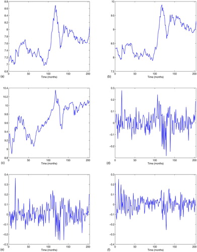
Table 3. True value and fitted value at points.

Sequence	ADF statistic	p-value	Conclusion
$p_{1t}$	−1.8774	0.6632	nonstationary
$p_{2t}$	−1.7991	0.7028	nonstationary
$p_{3t}$	−2.5853	0.2886	nonstationary
$r_{1t}$	−7.5507	0.0000	stationary
$r_{2t}$	−12.5946	0.0000	stationary
$r_{3t}$	−12.6409	0.0000	stationary

Source: The Authors.

To establish the empirical relationship among the series of SHSI, SZCI and HSI, similar to Tsay (2005) who considered the linear relationship between the one-year Treasury constant maturity rate and the three-year Treasury constant maturity rate, we first fit a simple linear regression model based on the above results of Granger causality test (6) $$p_{3t}=a_0+a_1{p}_{1t}+a_2{p}_{2t}+u_t.$$(6)

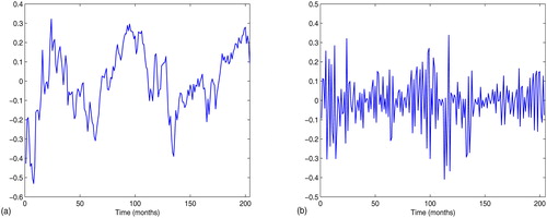
As a result, the least-square estimates of a₀, a₁ and a₂ are 5.7663(0.2807), −0.1514(0.0905) and 0.5835(0.0590), respectively. The adjusted R-squared is 0.6290, and the values of F-statistic and Durbin-Waston statistic are 261.9054 and 0.1617. By comparing these results with those from standard linear model, we might suspect that the considered model might be nonlinear. To this end, we examine the residual series derived from (6) and find that it does depend on time; see Figure 2a. Therefore, we have sufficient reasons to fit the following nonparametric model: (7) $$p_{3t}=f(p_{1t},p_{2t})+u_t.$$(7)

Figure 2. Residual graphs: (a) The residual plot of model (6(6) $$p_{3t}=a_0+a_1{p}_{1t}+a_2{p}_{2t}+u_t.$$(6) ); (b) The residual plot of model (7(7) $$p_{3t}=f(p_{1t},p_{2t})+u_t.$$(7) ). Source: The Authors.

The local linear estimator $\widehat{f}(·,·)$ is computed based on the optimal bandwidth matrix $H_{\mathit{opt}}=\left(\begin{array}{cc}0.325& 0\\ 0& 0.300\end{array}\right),$ which is selected by the AIC bandwidth matrix selector described in Section 2.2. The residual plot in Figure 2b shows that the errors are close to normal, thus the local linear estimates are expected to be efficient.

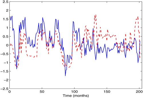
To further study the effect of SHCI and SZCI on HSI, we computer the first-order partial derivatives of HSI over SHCI and SZCI, which are depicted in Figure 3 (solid curve represents the derivative of $p_{3t}$ with respect to $p_{1t},$ dashed curve represents the derivative of $p_{3t}$ with respect to $p_{2t}$). We can observe from Figure 3 that the influence of SHCI and SZCI to HSI appears to be a strong nonlinear characteristics. Meanwhile, this effect presents a significant period, and it can be roughly divided into two periods: the first period of the trading months from 1 to 104 (The corresponding calendar months are from January, 1998–July, 2006.), the effect of SZCI $p_{2t}$ and HSI $p_{3t}$ on HSI $p_{3t}$ is synchronous. The positive and negative roles appear alternately; the second period of the trading months from 105 to 204 (The corresponding calender months are from August, 2006 to December, 2014.), the SZCI $p_{2t}$ shows a strong positive impact on HSI $p_{3t},$ while the SHCI $p_{1t}$ has a negative impact on HSI $p_{3t}.$ Therefore, one might conclude that three is a nonparametric cointegration relationship among SHCI, SZCI and HSI. Finally, to support our conclusions statistically, we consider the testing null hypothesis ${\mathbf{H}}_0:f(·,·)=\eta ,$ and the testing procedure described in Section 2.2 is used with the bootstrap sampling 1000 times. As a result, the p-value is less than 0.001. Thus, this test result further supports our finding that the relationship among SHCI, SZCI and HSI can be described by a nonparametric cointegration model.

Figure 3. The estimated first-order partial derivative: solid curve represents the derivative of $p_{3t}$ with respect to $p_{1t},$ dashed curve represents the derivative of $p_{3t}$ with respect to $p_{2t}.$ Source: The Authors.

5. Conclusion and discussion

In this article, we developed a multivariate cointegration time series model to model nonlinear and nonstationary time series. A nonparametric local linear kernel smoothing method was proposed for estimating the model function. Then, we adapted a testing procedure for testing misspecification, based on the comparison of the RSS and suggested using a bootstrap to estimate the p-value. Furthermore, We obtained some insights about the modeling methods via some Monte Carlo experiments and demonstrated that the local linear estimator performed well. Finally, the usefulness of the considered model was demonstrated by an empirical application.

Some further research can be conducted in several directions. Firstly, we would consider models allowing ${\epsilon }_i$ to be heteroscedastic, and it would be of interest to extend this study to models containing lagged dependent variables. Secondly, an extension of the semiparametric modeling and estimation to multivariate cointegration time series models would also be interesting. Thirdly, the predictive utility of multivariate cointegration time series models needs further investigation.

Disclosure statement

No potential conflict of interest was reported by the authors.

Additional information

Funding

We would like to express our gratitude to the editors and three anonymous referees whose comments and suggestions have contributed to the improvement of the paper. Zhao’s research is supported by National Natural Science Foundation of China (11701286, 11971235), and Natural Science Foundation of Jiangsu Province (BK20171073). Ye’s research is supported by National Natural Science Foundation of China (11961038).

References

- Bae, Y., Kakkar, V., & Ogaki, M. (2006). Money demand in Japan and nonlinear cointegration. Journal of Money, Credit, and Banking, 38(6), 1659–1667. doi:10.1353/mcb.2006.0076
- Breitung, J. (2002). Nonparametric tests for unit roots and cointegration. Journal of Econometrics, 108(2), 343–363. doi:10.1016/S0304-4076(01)00139-7
- Cai, Z. (2002). A two-stage approach to additive time series models. Statistica Neerlandica, 56(4), 415–433. doi:10.1111/1467-9574.00210
- Cai, Z. (2007). Trending time-varying coefficient time series models with serially correlated errors. Journal of Econometrics, 136(1), 163–188. doi:10.1016/j.jeconom.2005.08.004
- Cai, Z., & Tiwari, R. C. (2000). Application of a local linear autoregressive model to BOD time series. Environmetrics, 11(3), 341–350. doi:10.1002/(SICI)1099-095X(200005/06)11:3<341::AID-ENV421>3.0.CO;2-8
- Campbell, J. Y. (1987). Stock returns and the term structure. Journal of Financial Economics, 18(2), 373–399. doi:10.1016/0304-405X(87)90045-6
- Campbell, J. Y. (1991). A variance decomposition for stock returns. The Economic Journal, 101(405), 157–179. doi:10.2307/2233809
- Campbell, J. Y., & Ammer, J. (1993). What moves the stock and bond markets? A variance decomposition for long-term asset returns. The Journal of Finance, 48(1), 3–37. doi:10.1111/j.1540-6261.1993.tb04700.x
- Campbell, J. Y., & Shiller, R. J. (1991). Yield spreads and interest rate movements, a bird’s eye view. The Review of Economic Studies, 58(3), 495–514. doi:10.2307/2298008
- Chen, M. H. (2003). Risk and return: CAPM and CCAPM. The Quarterly Review of Economics and Finance, 43(2), 369–393. doi:10.1016/S1062-9769(02)00125-4
- Cross, E., & Worden, K. (2011). Approaches to nonlinear cointegration with a view towards applications in SHM. Journal of Physics: Conference Series, 305(1), 012069. doi:10.1088/1742-6596/305/1/012069
- Dickey, D. A., & Fuller, W. A. (1979). Distributions of the estimators for autoregressive time series with a unit root. Journal of the American Statistical Association, 74(366), 427–481. doi:10.2307/2286348
- Elliot, G., Rothenberg, T. J., & Stock, J. H. (1996). Efficient tests for an autoregressive unit root. Econometrica, 64, 813–836. doi:10.2307/2171846
- Fama, E. F. (1984). The information in the term structure. Journal of Financial Economics, 13(4), 509–528. doi:10.1016/0304-405X(84)90013-8
- Fama, E., & Schwert, G. W. (1997). Asset returns and in ation. Journal of Financial Economics, 5, 115–146.
- Fan, J., & Gijbels, I. (1996). Local polynomial modelling and its application. London: Chapman and Hall.
- Fan, J., Zhang, C., & Zhang, J. (2001). Generalized likelihood ratio statistics and Wilks phenomenon. The Annals of Statistics, 29(1), 153–193. doi:10.1214/aos/996986505
- Ghosh, S., & Kanjilal, K. (2014). Co-movement of international crude oil price and Indian stock market: Evidences from nonlinear cointegration tests. Energy Economics, 53, 111–117. doi:10.1016/j.eneco.2014.11.002
- Hadi, M. D., Katircioğlu, S., & Adaoglu, C. (2019). The vulnerability of tourism firms’ stocks to the terrorist incidents. Current Issues in Tourism, 1–15. doi:10.1080/13683500.2019.1592124
- Jawadi, F., Bruneau, C., & Sghaier, N. (2009). Nonlinear cointegration relationships between non-life insurance premiums and financial markets. Journal of Risk and Insurance, 76(3), 753–783. doi:10.1111/j.1539-6975.2009.01314.x
- Johansen, S. (1988). Statistical analysis of cointegrating vectors. Journal of Economic Dynamics and Control, 12(2-3), 231–254. doi:10.1016/0165-1889(88)90041-3
- Johansen, S. (1991). Estimation and hypothesis testing of cointegrating vectors in Gaussian autoregressive models. Econometrica, 59(6), 1551–1580. doi:10.2307/2938278
- Johansen, S. (1995). Likelihood-based inference in cointegrated vectors autoregressive models. Oxford: Oxford University Press.
- Johansen, S., & Juselius, K. (1990). Maximum likelihood estimation and inference on cointegration-with applications to the demand for money. Oxford Bulletin of Economics and Statistics, 52(2), 169–210. doi:10.1111/j.1468-0084.1990.mp52002003.x
- Juhl, T. (2005). Functional-coefficient models under unit root behaviour. The Econometrics Journal, 8(2), 197–213. doi:10.1111/j.1368-423X.2005.00160.x
- Kanas, A. (2003). Non-linear cointegration between stock prices and dividends. Applied Economics Letters, 10(7), 401–405. doi:10.1080/1350485022000044020
- Karlsen, H. A., Myklebust, T., & Tjøstheim, D. (2007). Nonparametric estimation in a nonlinear cointegration type model. The Annals of Statistics, 35(1), 252–299. doi:10.1214/009053606000001181
- Katircioğlu, S., Alkhazaleh, M. M. H., & Katircioğlu, S. (2018). Interactions between oil prices and financial sectors’ performances: empirical evidence from Amman Stock Exchange. Environmental Science and Pollution Research, 25(33), 33702–33708. 2018, doi:10.1007/s11356-018-3311-5
- Katircioğlu, S., & Zabolotnov, A. (2019). Role of financial development in economic globalization: evidence from global panel. Applied Economics Letters, 1–7. doi:10.1080/13504851.2019.1616058
- Kwiatkowski, D., Phillips, P. C. B., Schmidt, P., & Shin, Y. (1992). Testing the null hypothesis of stationarity against the alternative of a unit root: How sure are we that economic time series have a unit root? Journal of Econometrics, 54(1-3), 159–178. doi:10.1016/0304-4076(92)90104-Y
- Liang, Z., Lin, Z., & Hsiao, C. (2015). Local linear estimation of a nonparametric cointegration model. Econometric Reviews, 34(6-10), 882–906. doi:10.1080/07474938.2014.956610
- Ma, Y., & Kanas, A. (2004). Intrinsic bubbles revisited: Evidence from nonlinear cointegration and forecasting. Journal of Forecasting, 23(4), 237–250. doi:10.1002/for.909
- Ng, S., & Perron, P. (2001). LAG length selection and the construction of unit root tests with good size and power. Econometrica, 69(6), 1519–1554. doi:10.1111/1468-0262.00256
- Pesaran, H. H., & Shin, Y. (1998). Generalized impulse response analysis in linear multivariate models. Economics Letters, 58(1), 17–29. doi:10.1016/S0165-1765(97)00214-0
- Pesaran, M. H., Shin, Y., & Smith, R. J. (2001). Bounds testing approaches to the analysis of level relationships. Journal of Applied Econometrics, 16(3), 289–326. doi:10.1002/jae.616
- Phillips, P. C. B., & Perron, P. (1988). Testing for a unit root in time series regression. Biometrika, 75(2), 335–346. doi:10.1093/biomet/75.2.335
- Rezgallah, H., Özataç, N., & Katircioğlu, S. (2019). The impact of political instability on risk-taking in the banking sector: International evidence using a dynamic panel data model (System-GMM). Managerial and Decision Economics, 40(8), 891–906. doi:10.1002/mde.3075i
- Sadorsky, P. (2003). The macroeconomic determinants of technology stock price volatility. Review of Financial Economics, 12(2), 191–205. doi:10.1016/S1058-3300(02)00071-X
- Shaeri, K., & Katircioğlu, S. (2018). The nexus between oil prices and stock prices of oil, technology and transportation companies under multiple regime shifts. Economic Research-Ekonomska Istraživanja, 31(1), 681–702. doi:10.1080/1331677X.2018.1426472
- Tsay, R. S. (2005). Analysis of financial time series. New York: John Wiley & Sons.
- Tschernig, R., & Yang, L. (2000). Nonparametric lag selection for time series. Journal of Time Series Analysis, 21(4), 457–487. doi:10.1111/1467-9892.00193
- Wang, Q., & Phillips, P. C. B. (2009a). Asymptotic theory for local time density estimation and nonparametric cointegrating regression. Econometric Theory, 25(3), 710–738. doi:10.1017/S0266466608090269
- Wang, Q., & Phillips, P. C. B. (2009b). Structural nonparametric cointegrating regression. Econometrica, 77(6), 1901–1948.
- Yao, Q., & Tong, H. (1994). On subset selection in non-parametric stochastic regression. Statistica Sinica, 4(1), 51–70. doi:10.5705/ss.202016.0369
- Ye, X. G., Lin, J. G., Zhao, Y. Y., & Hao, H. X. (2015). Two-step estimation of the volatility functions in diffusion models with empirical applications. Journal of Empirical Finance, 33, 135–159. doi:10.1016/j.jempfin.2015.05.001