Dynamic relationship between the stock market and macroeconomy in China (1995–2018): new evidence from the continuous wavelet analysis

Abstract

This article examines the relationship between the stock market and three widely used macroeconomic variables, namely industrial production growth, inflation, and long-term interest rate in China. We use the continuous wavelet analysis to investigate the correlations and lead–lag relationships between them in the time–frequency domain by covering a period of 1995M01-2018M04. Our findings show the positive relationship between stock returns and industrial production growth and between stock returns and inflation. Notably, we find that stock returns and long-term interest rate are negatively correlated in short and medium terms, while they are positively correlated in the long term. The puzzling positive correlation between stock returns and interest rate as well as the mixed lead–lag relationships suggest that the Chinese stock market is quite undeveloped. There are breakdowns of the link between the stock market and macroeconomy. Neither the stock return can be used as a leading indicator of the macroeconomy nor the real economy could predict the booms or busts of the Chinese stock market.

Keywords:

• Stock market
• macroeconomy
• China
• continuous wavelet analysis
• time–frequency domain

Subject Classification Codes:

• C22
• E44
• O16

1. Introduction

The interactive relationship between the stock market and macroeconomy has attracted attention worldwide for a long time. Since the macroeconomy is the fundamental of the stock market performance, some studies investigate whether the stock price can be viewed as a leading indicator of the real economy (Borjigin et al., 2018; Croux & Reusens, 2013; Fama, 1990; Gallegati, 2008; Naes, Skjeltorp, & Ødegaard, 2011; Pan & Mishra, 2018; Peiró, 2016; Schwert, 1990; Tiwari et al., 2015). On the other hand, some studies argue that since economic activities reflect the movement of stock prices, the economic variables could predict stock returns (Girardin & Joyeux, 2013; Humpe & Macmillan, 2009; Liu & Shrestha, 2008; Rapach, Wohar, & Rangvid, 2005), furthermore, predict the severe bear market (Chen, 2009; Wu & Lee, 2012, 2015). However, no conclusive results have been reached regarding the form and the causal direction of the relationship between them. Therefore, it is of importance to explore the interaction between the stock market and economic factors.

A number of previous studies focus on the mature stock markets in developed countries (Croux & Reusens, 2013; Fama, 1981; 1990; Humpe & Macmillan, 2009; Mukherjee & Naka, 1995; Peiró, 2016; Schwert, 1990). China drew attention in recent years with the rapid economic growth and financial development as well. Shanghai Stock Exchange (SHSE) and Shenzhen Stock Exchange (SZSE) were established in December 1990 and July 1991. The market capitalisation was RMB 294.35 billion and RMB 100.65 billion for SHSE and SZSE in July 1995 and reached RMB 32.79 trillion and RMB 22.35 trillion in May 2018, respectively.¹ Despite the rapidly expanding market capitalisation, the Chinese stock market is still immature and undeveloped due to the dominance of individual investors. With little investment knowledge and experience, individual investors trade like noise traders, who purely speculate and treat the market as a casino (De Bondt, Peltonen, & Santabárbara, 2011; Liu & Shrestha, 2008). In addition, the imperfect regulatory framework and social security system are attributed to the speculative behaviours of the stock market (Liu & Shrestha, 2008). Several studies have examined the existence of speculative bubbles in the Chinese stock market (Jiang et al., 2010; Li, 2017; Liu, Gu, & Xing, 2016; Sarno & Taylora, 1999).

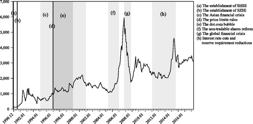
Figure 1 exhibits the SHSE composite index² during 1990M12-2018M04, displaying an upward with constant fluctuations. It reached 128 points in December 1990 and decreased from the highest 5955 points in October 2007 to 3082 points in April 2018. Five significant fluctuations can be observed during specified periods of 1992-1994, 2000-2002, 2005-2008, 2009-2012, and 2014-2016. The Chinese stock market witnessed volatilities at the early stage with the absence of price limits rules. During the end of the 1990s, the dot.com bubble came to fame in the US and had a great impact on the Chinese stock market. The most dramatic fluctuation occurred during 2005-2008. The Chinese stock market has entered the great bull market with the launch of non-tradable shares reform and the vigorous real economy since 2005. However, it suffered a significant and continuous decline after the outbreak of the US subprime crisis and the global financial crisis in 2008. The Chinese stock market began to rebound in 2009 since the government released several bailout policies, including the four trillion investment plan, the pro-active fiscal policy, and the moderately easy monetary policy. The most recent peak occurred in May 2015. China conducted several rounds of interest rate cuts and reserve requirement reductions to boost the real economy. The stock market overreacted from the stimulus and crashed in the second half of 2015.

Figure 1. SHSE composite index. Source: CEIC database.

China experienced great changes in economy and society in the past few decades. As an emerging market, the Chinese stock market still requires further development and regulation. It is well known for its dominance of individual investors and volatilities. Therefore, it is of significance to investigate the dynamic interaction between the stock market and macroeconomy in China. This article intends to shed some light on the relationship between the stock market and macroeconomy in China and contributes to the existing research in three ways. Firstly, we seek to find out a reliable outcome in the case of China, a typical emerging country with undeveloped stock market, providing some valuable experience and explanations for other emerging economies. Secondly, we take into account time variations in the interaction between the stock market and real economy. Instead of full sample causality, we aim to extend the time-varying analysis and offer new findings by covering a relatively long-time span from 1995M01 to 2018M04. Thirdly, the continuous wavelet analysis is used to provide detailed and thorough empirical analysis. As a popular method exploring the relationship between two variables, the continuous wavelet analysis expands time series to a time–frequency space in such a way that the correlation and the lead–lag relationship can be observed. Hence, it could be used appropriately to conduct the time-varying analysis and explore the lead–lag relationship between the stock market and economic factors (Aguiar-Conraria & Soares, 2014).

The remainder of this paper is structured as follows. Section 2 provides a brief summary of recent literature. Section 3 describes the empirical model and data. The continuous wavelet analysis is used to model the correlation and the lead–lag relationship between the stock market and macroeconomic variables. Section 4 presents the empirical evidence and the robustness check. The final section concludes.

2. Literature review

2.1. Relationship between the stock market and macroeconomy

There has been ample interesting work examining the relationship between the stock market and macroeconomy. A number of researches do not find the causal relationship between the stock market and macroeconomy, while some articles reveal a significant causality. It is worth noting that the conclusions reached by the first group of papers are mainly addressed in emerging markets, while the second group of papers is mainly conducted in developed countries.

Regarding the first strand of papers, Gallegati (2008) investigated the relationship between stock returns and aggregate economic activity in the US. Empirical results indicated a slight anticorrelation and stock returns leading aggregate economic activity only at low frequencies based on the maximum overlap discrete wavelet transform (MODWT) and wavelet cross-correlation analysis. Focusing on the Chinese stock market, Girardin & Joyeux (2013) found that the influence of macroeconomic variables on the long-run volatility is limited, with a noteworthy disconnect form the real economy using the GARCH-MIDAS approach. Chen & Chiang (2016) investigated the economic forces that determine China’s stock returns. There is no significant evidence that stock returns can be predicted by the growth of dividend yields. However, some articles showed that the stock price is cointegrated with a set of macroeconomic variables while the stock price is not a leading indicator for macroeconomy. Kwon & Shin (1999) addressed this subject using the cointegration test and the vector error correction model in Korea. The similar conclusions were reached in New Zealand with Johansen cointegration test and Granger-causality test (Gan et al, 2006).

In the second group of papers, stock market and macroeconomy are examined to be correlated or stock prices contain predictive power for macroeconomy. Schwert (1990) found out a strong positive relationship between stock returns and future production growth rates in the US during 1889–1988. The stock market is cointegrated with a group of macroeconomic variables by employing the vector error correction model in Japan (Mukherjee & Naka, 1995). Aylward & Glen (2000) found that stock prices can predict future economic activities but with substantial variation across countries. The influence of stock price on the future real economy in the G7 countries is significantly stronger than that in emerging countries. Croux & Reusens (2013) revealed that the predictive power of the stock price for the future GDP is predominantly present at the low frequencies in the G7 countries by decomposing the Granger causality in the frequency domain. Peiró (2016) suggested that industrial production and long-term interest rates are significant variables explaining the movements in stock prices in France, Germany, and the United Kingdom. In the case of China, the cointegrating relationship does exist between stock prices and macro-economic variables using the heteroscedastic cointegration analysis (Liu & Shrestha, 2008). Besides, Borjigin et al. (2018) showed that the nonlinear Granger causality is stronger and stock prices can lead the macroeconomy, compared with the static nonlinear Granger causality test.

2.2. Theoretical basis

Among the above articles, the theoretical basis of the relationship between the stock market and macroeconomy has been widely investigated. On the one hand, the Arbitrage Pricing Theory (Ross, 1976) links stock prices and macroeconomic variables using multiple risk factors, the macroeconomic ones included to explain asset returns. The APT suggests that changes in certain macroeconomic variables cause changes in systematic risk factors and affect stock returns. Several empirical studies based on the APT revealed the significant short-term correlation between the stock market and macroeconomy (Fama, 1981; 1990; Ferson & Harvey, 1991; Schwert, 1990). On the other hand, the Present Value Model (PVM) is also employed as an alternative to explain the nexus between them with certain inconsistencies with the APT. The PVM (Shiller, 1980) suggested that the stock price is dependent on future expected cash flows and future discount rate. The changes in any macroeconomic factor that affect the two main determinants influence the stock price. In contrary to the short-term relations supported by the APT, several empirical studies addressed the subject based on the PVM mainly in the long run (Chen, Roll, & Ross, 1986; Croux & Reusens, 2013; Humpe & Macmillan, 2009; Peiró, 2016).

2.3. Empirical evidence

Following the spirit of the PVM, we select the macroeconomic factors that are closely related to future cash flows and discount rates, namely, industrial production, interest rate, and inflation.

Firstly, the stock market performance is examined to be positively correlated with industrial production, which is widely used to represent future cash flows. Fama (1981; 1990) and Schwert (1990) concluded that the growth of industrial production explains a large fraction of the movement of stock returns. A large number of empirical studies arrived to the similar results later (Bekhet & Matar, 2013; Borjigin et al., 2018; Cheung & Ng, 1998; Engle, Ghysels, & Sohn, 2013; Gallegati, 2008; Girardin & Joyeux, 2013; Humpe & Macmillan, 2009; Lee, 1992; Liu & Shrestha, 2008; Mukherjee & Naka, 1995; Peiró, 2016; Tiwari et al., 2015). Secondly, the changes in interest rates affect stock prices through the discount rate. Specifically, the discount rate increases with higher interest rates. Furthermore, stock prices decrease. In addition, interest rate cuts also stimulate the real economy and drive more money flooding into the equity market, increasing the prices of assets eventually. The negative relation between interest rates and stock prices was examined by several empirical studies (Andrieș, Ihnatov, & Tiwari, 2014; Bekhet & Matar, 2013; Bulmash & Trivoli, 1991; Chen, Roll, & Ross, 1986; Fama, 1981; Humpe & Macmillan, 2009; Lee, 1992; Liu & Shrestha, 2008; Mukherjee & Naka, 1995; Peiró, 2016). However, Mukherjee & Naka (1995) found out the positive relationship between stock prices and short-term interest rates in Japan. They argued that compared to the long-term interest rate, the short-term interest rate is less suitable to be used as a proxy of the discount rate. Thirdly, the relationship between stock price and inflation is ambiguous. On the one hand, higher inflation increases the discount rate, thus lowers the stock price. However, the decrease of discount rates could also be set off by the build-ups in cash flows from higher inflation rates. On the other hand, since expected inflation lowers the expected return of money, the demand for money decreases and the demand for equity increases accordingly, leading to higher stock price (Marshall, 1992). The current studies mainly concluded that stock prices are negatively correlated with the inflation rate (Borjigin et al., 2018; Girardin & Joyeux, 2013; Humpe & Macmillan, 2009; Liu & Shrestha, 2008; Mukherjee & Naka, 1995).

In summary, the current literature has studied the nexus between the stock market and macroeconomy using various individual economic variables, samples, and methodologies. However, the exact nature of the relationship between them is not conclusive. To the best of our knowledge, a number of studies have conducted the empirical analysis in the time or frequency domain, and only a few papers provide with evidence in the time–frequency window. In fact, the relationship between the stock market and macroeconomy is potentially dynamic and non-linear. Therefore, following the above arguments, this article re-examines the time-varying relationship between stock returns and several macroeconomic variables including industrial production, interest rate, and inflation.

3. Methodology and Data

3.1. Continuous wavelet analysis

In this study, we use the continuous wavelet analysis, a popular tool to extend the time–frequency analysis between two variables. It has been proposed as an alternative to the well-known Fourier analysis, a frequency domain technique with the drawback of losing time information (Aguiar-Conraria, Azevedo, & Soares, 2008; Aguiar-Conraria & Soares, 2011; 2014). First, it possesses advantages over conventional time domain and frequency domain approaches by estimating the spectral characteristics of a time series as a function of time. It extracts localised information in a time–frequency window, assessing how its different periodic components change over time (Aguiar-Conraria & Soares, 2014; Li et al., 2015). In other words, it describes how the relationship between two variables develops over time and varies across different frequency bands in a highly intuitive way. Second, it provides information about the lead–lag relationship between two variables. It, therefore, has been widely used to identify the leading indicator between two interactive factors or estimate the co-movement and causality between two variables (Aloui, Hkiri, & Nguyen, 2016; Chen, Chen, & Tseng, 2017; Loh, 2013; Tiwari, 2013). Third, it does not require the two time series to be stationary or cointegrated, which exhibits a major advantage of widely accommodating economic series, regardless of stationary properties (Aguiar-Conraria, Azevedo, & Soares, 2008; Aguiar-Conraria & Soares, 2011, 2014; Cazelles et al., 2007).

The continuous wavelet analysis involves the following procedures as well as associated wavelet tools including the continuous wavelet transform, wavelet power spectrum, wavelet coherency, and phase-difference. First, the continuous wavelet transform expands the time series into a time–frequency plane by mapping the original series into a function of time and frequency. Furthermore, the cross-wavelet transform is defined as a product of the continuous wavelet transform of two time series. Second, the wavelet power spectrum and the cross-wavelet spectrum are applied. The former depicts the local variance of a time series, and the latter describes the local covariance of two time series at each time and frequency. In this paper, the wavelet power spectrums measure the localised volatilities of the stock market and macroeconomy, revealing the potential existence of structural breaks in the underlying series. Third, we proceed with the wavelet coherency and phase-difference. The wavelet coherency can be seen as a localised correlation coefficient in the time–frequency space. It is analogous with the Pearson’s correlation coefficient in the time domain and the dynamic correlation coefficient in the frequency domain with a value between 0 and 1. It describes the correlation between x_t and y_t in a three-dimensional way, considering the time and frequency components, and the strength of correlation as well (Loh, 2013). The phase-difference depicts synchronisations and delays between x_t and y_t. It is calculated to distinguish between positive and negative correlations and lead–lag relationship since the value of the wavelet coherency is always positive.

As a time–frequency method, the continuous wavelet analysis can provide more detailed empirical results compared to other conventional time series analysis. Hence, it can extend a thorough and elaborated analysis of the dynamic correlation between the stock market and macroeconomy. The continuous wavelet analysis used in this article has been developed by Aguiar-Conraria and Soares (2014). Besides, the continuous wavelet analysis performed in the present paper is processed by the MATLAB ASToolbox developed by Aguiar-Conraria and Soares (2014).

3.1.1. The continuous wavelet transform

Based on a mother wavelet $\psi ,$ a family ${\psi }_{\tau ,s}$ of “wavelet daughters” is defined as: (1) $${\psi }_{\tau ,s}\left(t\right):=\frac{1}{\sqrt{\left|s\right|}}\psi \left(\frac{t-\tau }{s}\right),\tau ,s\in \mathbb{R},s\ne 0$$(1) where $\tau$ is a translation parameter that controls the location of the wavelet, and $s$ is a scaling factor that defines its width. In this study, the most popular Morlet wavelet is chosen as the mother wavelet, which is given as: (2) $$\psi \left(t\right)={\pi }^{-\frac{1}{4}}\hspace{0.17em}\text{exp}\hspace{0.17em}\left(\mathrm{i}{\varpi }_0\mathrm{t}\right)\hspace{0.17em}\text{exp}\hspace{0.17em}\left(-\frac{1}{2}{t}^2\right)$$(2) where ${\int }_{-\infty }^{\infty }{\left|\psi (t)\right|}^{2}dt<\infty ,$ and ${\int }_{-\infty }^{\infty }\psi (t)dt=0.$

Based on the mother wavelet, the continuous wavelet transform is defined as (3) $$W_{x;\psi }\left(\tau ,s\right)={\int }_{-\infty }^{\infty }x\left(t\right)\frac{1}{\sqrt{\left|s\right|}}{\psi }^{*}\left(\frac{t-\tau }{s}\right)dt$$(3) where * denotes the complex conjugation of the Morlet wavelet. The continuous wavelet transform decomposes the original series into a function of $\tau$ and $s,$ thus the time series is expanded into a time–frequency space. When the wavelet $\psi (t)$ is complex-valued, the wavelet transform $W_x(\tau ,s)$ is also complex-valued and can be decomposed into its real part $\mathfrak{R}\left\{W_x(\tau ,s)\right\}$ and its imaginary part $\mathfrak{I}\left\{W_x(\tau ,s)\right\},$ or in its amplitude, $\left|W_x(\tau ,s)\right|$ and its phase, ${\varphi }_x(\tau ,s):W_x(\tau ,s)=\left|W_x(\tau ,s)\right|\hspace{0.17em}\text{exp}\hspace{0.17em}(i{\varphi }_x(\tau ,s)).$

3.1.2. The power of wavelet and cross-wavelet

Following the continuous wavelet transform, the wavelet power spectrum is given as: (4) $$WP{S}_x\left(\tau ,s\right)={\left|W_x\left(\tau ,s\right)\right|}^2$$(4)

Furthermore, the cross-wavelet transform and the cross-wavelet power spectrum of the two series are extended. The cross-wavelet transform of the two time series, $x(t)$ and $y(t)$ is defined as: (5) $$W_{xy}\left(\tau ,s\right)=W_x\left(\tau ,s\right)W_y^{*}\left(\tau ,s\right)$$(5) where $W_x(\tau ,s)$ and $W_y(\tau ,s)$ are the continuous wavelet transforms of time series $x(t)$ and $y(t).$ When $y=x,$ the wavelet power spectrum is given as $W_{xx}(\tau ,s)={\left|W_x(\tau ,s)\right|}^2={(\mathit{WPS})}_x(\tau ,s).$ The cross-wavelet power is given as (6) $$XW{P}_{xy}\left(\tau ,s\right)=\left|W_{xy}\left(\tau ,s\right)\right|$$(6)

In general, the wavelet power spectrum of one time series presents the local variance, while the cross-wavelet power spectrum measures the local covariance of two time series at each time and frequency.

3.1.3. The wavelet coherency and the phase-difference

Based on the wavelet power spectrum and the cross-wavelet power, the wavelet coherency is conducted to investigate the dynamic correlation in the time–frequency domain. The complex wavelet coherency ${\varrho }_{xy}$ is given as: (7) $${\varrho }_{xy}=\frac{S\left(W_{xy}\right)}{{\left[S\left({\left|W_x\right|}^2\right)S\left({\left|W_y\right|}^2\right)\right]}^{\frac{1}{2}}}$$(7) where $S$ denotes a smoothing operator in both time and scale. The wavelet coherency is defined as the absolute value of the complex wavelet coherency: (8) $$R_{xy}=\frac{\left|S\left(W_{xy}\right)\right|}{{\left[S\left({\left|W_x\right|}^2\right)S\left({\left|W_y\right|}^2\right)\right]}^{\frac{1}{2}}},\text{with}0\le R_{xy}\le 1$$(8)

However, we are not able to differentiate the positive or negative correlation through the wavelet coherency since its value is always positive. Therefore, the phase-difference is applied to reveal the positive or negative correlation and lead–lag interaction between two time series. The complex wavelet coherency ${\varrho }_{xy}$ can be expressed in polar form, as ${\varrho }_{xy}=\left|{\varrho }_{xy}\right|\hspace{0.17em}\text{exp}\hspace{0.17em}(i{\varphi }_{xy}).$ The angle ${\varphi }_{xy}$ of the complex coherency is the phase-difference³, which is given as: (9) $${\varphi }_{xy}={\hspace{0.17em}\text{tan}\hspace{0.17em}}^{-1}\left(\frac{\mathfrak{I}\left(S\left(W_{xy}\right)\right)}{\mathfrak{R}\left(S\left(W_{xy}\right)\right)}\right),\text{with}{\varphi }_{xy}\in [-\pi ,\pi ]$$(9)

When ${\varphi }_{xy}\in \left(0,\frac{\pi }{2}\right)$ and ${\varphi }_{xy}\in \left(-\frac{\pi }{2},0\right),$ $x(t)$ and $y(t)$ move in phase (similarly to positive correlation), and the former indicates that $x(t)$ leads $y(t),$ while the latter indicates that $y(t)$ leads $x(t).$ When ${\varphi }_{xy}\in \left(-\pi ,-\frac{\pi }{2}\right)$ and ${\varphi }_{xy}\in \left(\frac{\pi }{2},\pi \right),$ $x(t)$ and $y(t)$ move anti-phase (similarly to negative correlation), and the former suggests that $x(t)$ leads $y(t),$ while the latter suggests the opposite. Besides, ${\varphi }_{xy}=0$ reveals the positive relationship between $x(t)$ and $y(t),$ and they move together. While ${\varphi }_{xy}=\pi$ or $-\pi$ reveals the negative and an antiphase relationship between $x(t)$ and $y(t).$

3.2. Data description

This article uses monthly data on the stock market performance and macroeconomic variables covering January 1995 to April 2018 with 280 observations. The closing prices of SHSE composite index of the last trading day in each month are used as a proxy of the stock market performance. We focus on the movement of stock prices (Stock) by taking the logarithmic difference of the price series, i.e. the stock returns. In terms of macroeconomy, we use the conventional macroeconomic variables including industrial production growth, inflation, and interest rate. The industrial production growth is obtained by taking the logarithmic difference of the monthly gross industrial production. The monthly Consumer Price Index (CPI) and five-year time deposit rate are used to measure the level of inflation (Inflation) and long-term interest rate (LIR). The data are selected from the CEIC database and the Hithink RoyalFlush Information Network Co., Ltd. Because of data availability, we restrict the sample to the 1995M01-2018M04 period for the variables of Stock, Inflation, and LIR, and the sample for IP is restricted to the 1995M01-2012M05 period.⁴ The descriptions of the variables and the original data sources are listed in Table 1.

Table 1. Descriptions of variables.

Variable	Description	Time period	Data source
Stock	Stock returns	1995M01-2018M04	CEIC database
IP	Industrial production growth	1995M01-2012M05	CEIC database, Hithink RoyalFlush Information Network Co., Ltd.
Inflation	Consumer Price Index (CPI)	1995M01-2018M04	CEIC database
LIR	Real five-year time deposit rate	1995M01-2018M04	CEIC database

Note: All the variables are logarithmic values and deflated with the base date as December 1994.

4. Empirical results

4.1. Wavelet power spectrum analysis

Figure 2 displays the wavelet power spectrum of stock returns, industrial production growth, inflation rate, and long-term interest rate. The horizontal axis depicts the time dimension, and the vertical axis presents the frequency dimension in time units (years). The vertical axis is separated into 5 frequency bands: 0–0.5 years, 0.5–1 years, 1–2 years, 2–4 years, and 4–8 years, corresponding to the volatilities in the very short term, short term, medium term, long term, and very long term. The colour represents the strength of power, ranging from blue (low power) to yellow (high power). The white lines show the maxima of the undulations of the wavelet power spectrum, providing information on the estimate of the cycle period. The cone of influence (COI) is given by a thick black line, which defines the regions affected by the edge effects. We mainly focus on the regions inside the COI.

Figure 2. (a.1) Stock, (a.2) Wavelet power spectrum of Stock; (b.1) IP, (b.2) Wavelet power spectrum of IP; (c.1) Inflation, (c.2) Wavelet power spectrum of Inflation; (d.1) LIR, (d.2) Wavelet power spectrum of LIR. Note: The black (gray) contour denotes the 5% (10%) significance level. The thick black contour represents the COI. The white lines show the maxima of the undulations of the wavelet power spectrum. Similarly hereinafter.

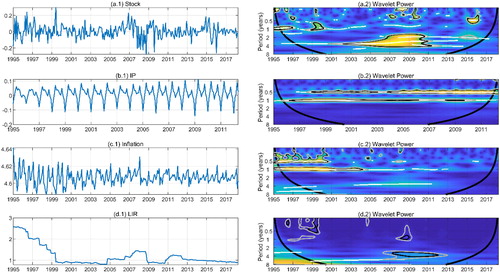
Figure 2 (a.2) shows volatilities of Stock are significant (at 5% significance level) in the 0-0.5 frequency band during 1996–1997, 2007–2008, and 2015–2016, in the 0.5–1 frequency band during 1996–1997 and 1999–2000, and in the 1–8 frequency band during 2002–2011. During 1996-2000, the stock returns experienced remarkable fluctuations from the Asian financial crisis and the dot.com bubble. In addition, the high power in the 1–8 frequency band during 2002–2011 could be attributed to the non-tradable shares reform, the vigorous real economy, and the global financial crisis. The volatilities of stock returns are also significant from 2007 to 2010 in the very short term. The significant volatilities across all the frequency bands during crisis periods indicate the deep and lasting impact of the global financial crisis on the Chinese stock market. The high power during 2015–2016 in the short term comes from the market crash in 2015, due to the overreaction to the quantitative easing policy.

The industrial production growth seems to present a cyclical pattern as shown in Figure 2 (b.1). Instead of significant volatilities, we focus on the periodical variation displayed by Figure 2 (b.2). We can observe two respective white lines on 0.5-year period during 1997-2012 and on 1-year period across all times. The periodicities of 0.5 year and 1 year can be explained by the production activities in a year. Since the Chinese Spring Festival is in February generally, the growth of industrial production drops significantly in February due to fewer production activities on holiday. It increases the most in March and declines gradually in the next few months until rebounds around October. Therefore, the industrial production growth experiences permanent periodical variations of six months and one year.

Figure 2 (c.1) shows that the volatilities of Inflation are more intense in the late 1990s. The volatilities of Inflation are significant (at 5% significance level) in the 0–0.5 frequency band over 1995–2001 and 2008, and in the 0.5–1 frequency band over 1996–2004. China launched the economic system reform in the early 1990s. The overheated investment that emerged from rapid economic growth generated large inflationary pressure. China undertook the tight monetary policy, and the inflation rate decreased afterward. The inflation rate was relatively high in the early 2000s since the contradiction of dual economic structure, experiencing volatilities during 1995-2004 in the lower frequency bands. In addition, the high power in 2008 in the very short term is mainly due to the stimulus economic policies in response to the global financial crisis.

The long-term interest rate displayed a clear downtrend indicated by Figure 2 (d.1). Figure 2 (d.2) shows significant (at 5% significance level) volatilities of LIR in the 0–0.5 frequency band over 1996–2000, in the 0.5–1 frequency band over 2008–2009, and in the 2–4 frequency band over 2007–2012, respectively. The nominal interest rate was relatively high in the 1990s.⁵ The significant volatilities in the 0–0.5 frequency band over 1996–2000 comes from a series of interest rate cuts in the late 1990s. Chinese government raised the interest rate several times in 2007 to deal with the excess liquidity, while reduced the interest rate in 2008 to boost the economy. Besides, the interest rate increased in 2010 and 2011 to prevent hot money from flooding into the real economy. Therefore, obvious fluctuations of LIR are observed in the short term over 2008-2009 and in the medium term over 2007–2012.

4.2. Wavelet coherency

Figure 3–5 present the wavelet coherency of stock returns and industrial production growth, inflation rate, and long-term interest rate, respectively. The vertical axis is decomposed into three frequency bands: 1–2 years, 2–4 years, and 4–8 years, corresponding to the coherencies in the short, medium, and long terms. The left-side subfigure displays the regions of significant coherency. The right-side subfigures present the results of phase differences, containing information on the correlation and lead–lag relationship in time–frequency domain.

Figure 3. Wavelet coherency between Stock and IP.

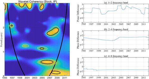
Figure 4. Wavelet coherency between Stock and Inflation.

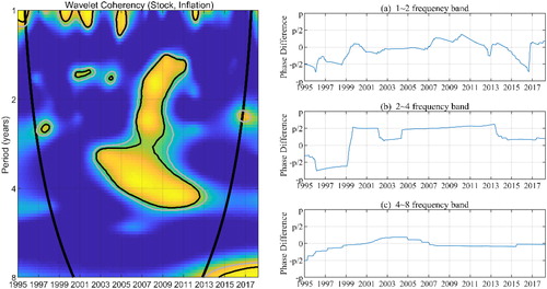
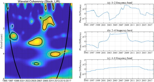
Figure 5. Wavelet coherency between Stock and LIR.

Figure 3 shows the significant coherency between stock returns and industrial production growth. In the 1–2 years frequency band, the coherency is significant during 1999–2002 and 2004–2005. In the former case, Stock and IP are positively correlated, while the lead–lag relationship changes from Stock leading to IP leading and changes back to Stock leading. However, in the latter case, ${\varphi }_{xy}\in \left(\frac{\pi }{2},\pi \right)$ indicates that Stock and IP are negatively correlated with IP leading, which is inconsistent with conventional theories and previous empirical analysis. During that period, investors had doubts about the Chinese stock market before the non-tradable shares reform. They held low expectations for the stock market performance despite the growing industrial production, which explains the puzzling negative correlation to an extent. In the 2–4 years frequency band and the 4-8 years frequency band, Stock and IP are positively correlated during 2005–2009 and 2005–2008. ${\varphi }_{xy}\in \left(0,\frac{\pi }{2}\right)$ means that Stock leads IP in the medium term and ${\varphi }_{xy}\in \left(-\frac{\pi }{2},0\right)$ suggests the opposite direction in the long term. The Chinese stock market was in a great bull market and the real economy was extremely vigorous before 2008. However, they both suffered huge losses from the global financial crisis, exhibiting a significant positive relationship.

As shown in Figure 4, the coherency is significant during 1999–2002, 2004–2005, and 2007–2013 in the 1–2 years frequency band. Stock and Inflation are positively correlated while the lead–lag relationship is quite mixed and less clear cut in the short term. In the 2–4 years frequency band, the coherency between Stock and Inflation is significantly positive with Stock leading during 2003–2005, and significantly negative with Inflation leading during 2009-2013. While during 2005-2009, ${\varphi }_{xy}=0$ indicates that they are positively correlated and move together. In the higher frequency, Stock and Inflation are also positively correlated. The lead–lag relationship changed from Stock leading to Inflation leading in 2007. The existing studies concluded the overwhelming negative relationship between stock returns and inflation. However, the above negative results demonstrate that the relationship between them is an empirical issue. The two variables interact through multiple ways and the positive or negative correlations vary in different samples. Higher inflation reduces the expected returns of money, motivating people to invest more money in the stock market. Stock prices and stock returns thence both go up.

We observe significant correlations between Stock and LIR during 2008-2012 in the 1-2 frequency band in Figure 5. ${\varphi }_{xy}\in \left(\frac{\pi }{2},\pi \right)$ indicates the negative relationship between them, and LIR is leading Stock. In the medium term, Stock and LIR are negatively correlated during 1997-1999 and 2003-2008. The former indicates that Stock leads LIR, while the latter suggests that Stock lags LIR. The negative relationship is supported by the existing articles. People tend to buy equity and require more returns compared to holding money at low interest rates. Therefore, the stock market may be likely to boom, and stock returns may increase. It is worth noting that ${\varphi }_{xy}\in \left(0,\frac{\pi }{2}\right)$ reveals the positive relationship between stock returns and long-term interest rate in the 4-8 years frequency band, which seems puzzling and contradictory. Three reasons are speculated to give a preliminary explanation. Firstly, the immaturity and speculation of the Chinese stock market may present in the long run, breaking the linkage between the stock market and macroeconomic variables. Secondly, China’s interest rate marketisation is still on process, and the five-year time deposit rate may not serve as a reliable proxy for future discount rate. Thirdly, the completeness of financial market in China is only not driven by stocks. In the long run, both stocks and debts help to complete the security market.

In summary, the above empirical results indicate the overall positive correlation between stock returns and industrial production growth and between stock returns and inflation in the time–frequency domain. However, stock returns and long-term interest rate are negatively correlated in the short and medium terms, while positively correlated in the long term. Moreover, the lead–lag relationships between stock returns and the three individual macroeconomic variables are quite mixed. Stock returns tend to lead industrial production growth in the medium term and lag in the long term. Long-term interest rate leads stock returns in the short term and lags in the long term. In other words, we do not find the leading indicator between stock returns and macroeconomic variables.

4.3. Robustness check

The above analyses provide time-varying coherencies between stock returns and macroeconomic variables during specific periods using the wavelet method. In addition, it is important to conduct a robustness check on whether the results still hold considering the full sample causality. Therefore, we use Granger causality tests to conduct the robustness causality check. Granger (1969) causality test examines whether the lags of one variable can be used to predict current values of another variable, which corresponds to the spirit of lead–lag relationship of the continuous wavelet analysis.

Firstly, we use ADF and PP methods to conduct the unit root tests. As shown in Table 2, all variables are stationary.

Table 2. Unit root test.

Variable	ADF		PP
	Statistic	p-value	Statistic	p-value
SR	−15.66030	0.0000***	−15.89310	0.0000***
dSR	−10.98214	0.0000***	−71.47052	0.0000***
IP	−2.698390	0.0761*	−12.57701	0.0000***
dIP	−8.691238	0.0000***	−31.54481	0.0001***
Inflation	−2.934325	0.0428**	−11.98811	0.0000***
dInflation	−20.14018	0.0000***	−40.60385	0.0001***
LIR	−3.298990	0.0159**	−3.217195	0.0200***
dLIR	−15.62520	0.0000***	−15.90220	0.0000***

Note: ***, **, and * indicate significance at the 1, 5, and 10 percent level respectively. Similarly hereinafter.

Secondly, we employ the Granger causality test to examine the causalities between stock returns and three macroeconomic variables. The lag structures are selected based on the SIC. As shown in Table 3, the null hypothesis of no Granger causality between stock returns and industrial production is not rejected. Besides, there is no Granger causality between stock returns and long-term interest rate in either direction. While we find the unidirectional causality from inflation to stock returns at the 10% significance level. However, 0.05 level is used as the significance level for it is more conservative than the 0.10 level. Therefore, the results of Granger causality test indicate that there is no causality between stock returns and macroeconomic variables. We reach the consistent conclusions based on the results of wavelet coherency from the perspective of lead-lag relationship. Notably, there are large regions of high coherency of stock returns and inflation, and the inflation tends to lead stock returns as shown in Figure 4. It supports the unidirectional causality from inflation to stock returns at the relatively weak significance level.

Table 3. Granger causality test.

H0	F-statistic	p-value	${\chi }^2$-statistic	p-value
Stock does not Granger-cause IP	0.68	0.5060	1.40	0.4964
IP does not Granger-cause Stock	1.43	0.2413	2.93	0.2305
Stock does not Granger-cause Inflation	1.41	0.2470	2.86	0.2390
Inflation does not Granger-cause Stock	2.84	0.0602*	5.78	0.0555*
Stock does not Granger-cause LIR	1.96	0.1629	1.98	0.1596
LIR does not Granger-cause Stock	0.27	0.6032	0.27	0.6008

However, Granger causality test may miss some contemporaneous correlation between variables if data are measured infrequently. Geweke (1982) proposed a measure of instantaneous correlation, which is calculated from the residuals of standard Granger causality tests, capturing “instantaneous feedback” (Dicle & Levendis, 2013). Table 4 reports the results of Geweke-type causality test. There is no Granger causality, instantaneous feedback, or total correlation between stock returns and industrial production growth and between stock returns and long-term interest rate. However, there is unidirectional causality from inflation to stock returns and the instantaneous feedback at the 10% significance level. The total correlation between them is significant at the 5% significance level. As discussed above in the Granger causality test, the results of Geweke-type causality test are also comparable and consistent with those of wavelet coherency, suggesting the absence of causal links between stock returns and macroeconomic variables. Moreover, large regions of high coherency of stock returns and inflation are consistent with the significant correlation between stock returns and inflation. Regarding the instantaneous feedback between them at relatively weak significance level, we also observe the co-movement between them during 2005–2009 based on the wavelet coherency in Figure 4.

Table 4. Geweke-type causality test.

		${\chi }^2$-statistic	p-value
Granger causation	Stock → IP	1.3826	0.5009
	IP → Stock	2.8860	0.2362
Instantaneous feedback	Stock ←→ IP	0.8911	0.3452
Total correlation	Stock, IP	5.1598	0.3967
Granger causation	Stock → Inflation	2.8271	0.2433
	Inflation →Stock	5.6825	0.0584*
Instantaneous feedback	Stock ←→ Inflation	2.9363	0.0866*
Total correlation	Stock, Inflation	11.4460	0.0432**
Granger causation	Stock → LIR	2.1668	0.3384
	LIR →Stock	0.3926	0.8218
Instantaneous feedback	Stock ←→ LIR	0.2209	0.6383
Total correlation	Stock, LIR	5.1598	0.3967

In summary, the robustness check indicates that the results of Granger causality test and Geweke-type causality test are consistent with those of the continuous wavelet analysis. The time-varying analysis on the interaction between stock returns and macroeconomic variables is still robust considering the full sample causality. We reach the same conclusion using the conventional Granger causality tests as we reach based on the continuous wavelet analysis. Stock returns cannot lead macroeconomic variables and vice versa.

5. Conclusions

Currently, the interactions between the stock market and macroeconomy remain to be well explained based on the previous theoretical and empirical research. In particular, whether the stock market can be viewed as a leading indicator of the real economy, or the stock returns could be predicted using the macroeconomic variables. This article analyzes the case of China, examining the nexus between stock returns and three individual macroeconomic factors, including industrial production growth, inflation, and long-term interest rate using monthly data during the period of 1995M01-2018M04. The continuous wavelet analysis is employed to conduct the time-varying analysis, which provides more information on the dynamic relationship between stock returns and the three important macroeconomic variables.

The empirical results reveal the following primary conclusions. Firstly, stock returns, inflation rate, and long-term interest rate all experienced significant volatilities in the late 1990s. Besides, stock returns and long-term interest rates both fluctuated dramatically during crisis periods. In contrast, industrial production growth exhibits periodical variations of six months and one year rather than significant fluctuations during specific periods. Secondly, stock returns are positively correlated with industrial production growth across all the frequency bands. In addition, stock returns and long-term interest rate are negatively correlated in the short and medium terms while positively correlated in the long term. The mixed correlation suggests certain breakdowns and instabilities of the link between stock market and the real economy, likely due to the immaturity and speculation of the Chinese stock market. Thirdly, the lead–lag relationships between stock returns and the three macroeconomic variables are all ambiguous. In general, the stock market could not be employed as a “national economic barometer” and the macroeconomic variables contain little predictive power for stock returns from the perspective of the continuous wavelet analysis.

The influence mechanism between the stock market and macroeconomy is quite complex and may be involved with many other factors and channels. This article provides empirical evidence from the perspective of dynamic correlation and lead–lag relationship based on the continuous wavelet analysis. Considerable work on this topic remains to be proceeded both on theoretical and empirical aspects. We leave this to further research.

Disclosure statement

No potential conflict of interest was reported by the author(s).

Additional information

Funding

This work was supported by China Scholarship Council; National Nature Science Foundation of China

Notes

1 The data was obtained from the CEIC database.

2 The SHSE composite index is generally used as the proxy of the Chinese stock market.

3 One has ${\varphi }_{xy}={\varphi }_x-{\varphi }_y,$ hence the name phase difference. The equation (9) holds after converting ${\varphi }_x-{\varphi }_y$ into an angle in the interval $[-\pi ,\pi ].$

4 Cazelles et al. (2008) claimed that the continuous wavelet analysis requires approximately 30-40 data points. In this study, we use 280 observations, which thus sufficient to extend the continuous wavelet analysis.

5 According to the People’s Bank of China, the call money interest rate was 10.98% and the five-year time deposit rate was 13.86% in January 1995.

References

- Aguiar-Conraria, L., Azevedo, N., & Soares, M. J. (2008). Using wavelets to decompose the time-frequency effects of monetary policy. Physica A: Statistical Mechanics and Its Applications, 387(12), 2863–2878. doi:10.1016/j.physa.2008.01.063
- Aguiar-Conraria, L., & Soares, M. J. (2011). Oil and the macroeconomy: Using wavelets to analyze old issues. Empirical Economics, 40(3), 645–655. doi:10.1007/s00181-010-0371-x
- Aguiar-Conraria, L., & Soares, M. J. (2014). The continuous wavelet transform: Moving beyond uni-and bivariate analysis. Journal of Economic Surveys, 28(2), 344–375. doi:10.1111/joes.12012
- Aloui, C., Hkiri, B., & Nguyen, D. K. (2016). Real growth co-movements and business cycle synchronization in the GCC countries: Evidence from time-frequency analysis. Economic Modelling, 52, 322–331. doi:10.1016/j.econmod.2015.09.009
- Andrieș, A. M., Ihnatov, I., & Tiwari, A. K. (2014). Analyzing time-frequency relationship between interest rate, stock price, and exchange rate through continuous wavelet. Economic Modelling, 41, 227–238. doi:10.1016/j.econmod.2014.05.013
- Aylward, A., & Glen, J. (2000). Some international evidence on stock prices as leading indicators of economic activity. Applied Financial Economics, 10(1), 1–14. doi:10.1080/096031000331879
- Bekhet, H. A., & Matar, A. (2013). Co-integration and causality analysis between stock market prices and their determinates in Jordan. Economic Modelling, 35, 508–514. doi:10.1016/j.econmod.2013.07.012
- Borjigin, S., Yang, Y., Yang, X., & Sun, L. (2018). Econometric testing on linear and nonlinear dynamic relation between stock prices and macroeconomy in China. Physica A: Statistical Mechanics and Its Applications, 493, 107–115. doi:10.1016/j.physa.2017.10.033
- Bulmash, S. B., & Trivoli, G. W. (1991). Time-lagged interactions between stock prices and selected economic variables. The Journal of Portfolio Management, 17(4), 61–67. doi:10.3905/jpm.1991.409351
- Cazelles, B., Chavez, M., Berteaux, D., Menard, F., Vik, J. O., Jenouvrier, S., & Stenseth, N. C. (2008). Wavelet analysis of ecological time series. Oecologia, 156 (2), 287–304. doi:10.1007/s00442-008-0993-2
- Cazelles, B., Chavez, M., De Magny, G. C., Guegan, J., & Hales, S. (2007). Time-dependent spectral analysis of epidemiological time-series with wavelets. Journal of the Royal Society Interface, 4(15), 625–636. doi:10.1098/rsif.2007.0212
- Chen, S. S. (2009). Predicting the bear stock market: Macroeconomic variables as leading indicators. Journal of Banking &Finance, 33(2), 211–223. doi:10.1016/j.jbankfin.2008.07.013
- Chen, M. P., Chen, W. Y., & Tseng, T. C. (2017). Co-movements of returns in the health care sectors from the US, UK, and Germany stock markets: Evidence from the continuous wavelet analyses. International Review of Economics & Finance, 49, 484–498. doi:10.1016/j.iref.2017.02.009
- Chen, X., & Chiang, T. C. (2016). Stock returns and economic forces-An empirical investigation of Chinese markets. Global Finance Journal, 30, 45–65. doi:10.1016/j.gfj.2016.01.001
- Chen, N. F., Roll, R., & Ross, S. (1986). Economic forces and the stock market. The Journal of Business, 59(3), 383–403. doi:10.1086/296344
- Cheung, Y., & Ng, L. K. (1998). International evidence on the stock market and aggregate economic activity. Journal of Empirical Finance, 5(3), 281–296.
- Croux, C., & Reusens, P. (2013). Do stock prices contain predictive power for the future economic activity? A Granger causality analysis in the frequency domain. Journal of Macroeconomics, 35, 93–103. doi:10.1016/j.jmacro.2012.10.001
- De Bondt, G. J., Peltonen, T. A., & Santabárbara, D. (2011). Booms and busts in China’s stock market: Estimates based on fundamentals. Applied Financial Economics, 21(5), 287–300. doi:10.1080/09603107.2010.530218
- Dicle, M. F., & Levendis, J. (2013). Estimating Geweke’s (1982) measure of instantaneous feedback. The Stata Journal: Promoting Communications on Statistics and Stata, 13(1), 136–140. doi:10.1177/1536867X1301300110
- Engle, R. F., Ghysels, E., & Sohn, B. (2013). Stock market volatility and macroeconomic fundamentals. Review of Economics and Statistics, 95(3), 776–797. doi:10.1162/REST_a_00300
- Fama, E. F. (1981). Stock returns, real activity, inflation, and money. The American Economic Review, 71(4), 545–565.
- Fama, E. F. (1990). Stock returns, expected returns, and real activity. The Journal of Finance, 45(4), 1089–1108. doi:10.1111/j.1540-6261.1990.tb02428.x
- Ferson, W. E., & Harvey, C. R. (1991). The variation of economic risk premiums. Journal of Political Economy, 99(2), 385–415. doi:10.1086/261755
- Gallegati, M. (2008). Wavelet analysis of stock returns and aggregate economic activity. Computational Statistics & Data Analysis, 52(6), 3061–3074. doi:10.1016/j.csda.2007.07.019
- Gan, C., Lee, M., Yong, H. H. A., & Zhang, J. (2006). Macroeconomic variables and stock market interactions: New Zealand evidence. Investment Management and Financial Innovations, 3(4), 89–101.
- Geweke, J. (1982). Measurement of linear dependence and feedback between multiple time series. Journal of the American Statistical Association, 77(378), 304–313. doi:10.1080/01621459.1982.10477803
- Girardin, E., & Joyeux, R. (2013). Macro fundamentals as a source of stock market volatility in China: A GARCH-MIDAS approach. Economic Modelling, 34, 59–68. doi:10.1016/j.econmod.2012.12.001
- Granger, C. W. (1969). Investigating causal relations by econometric models and cross-spectral methods. Econometrica, 37(3), 424–438. doi:10.2307/1912791
- Humpe, A., & Macmillan, P. (2009). Can macroeconomic variables explain long-term stock market movements? A comparison of the US and Japan. Applied Financial Economics, 19(2), 111–119. doi:10.1080/09603100701748956
- Jiang, Z. Q., Zhou, W. X., Sornette, D., Woodard, R., Bastiaensen, K., & Cauwels, P. (2010). Bubble diagnosis and prediction of the 2005–2007 and 2008–2009 Chinese stock market bubbles. Journal of Economic Behavior & Organization, 74(3), 149–162. doi:10.1016/j.jebo.2010.02.007
- Kwon, C. S., & Shin, T. S. (1999). Cointegration and causality between macroeconomic variables and stock market returns. Global Finance Journal, 10(1), 71–81. doi:10.1016/S1044-0283(99)00006-X
- Lee, B. S. (1992). Causal relations among stock returns, interest rates, real activity, and inflation. The Journal of Finance, 47(4), 1591–1603. doi:10.1111/j.1540-6261.1992.tb04673.x
- Li, C. (2017). Log-periodic view on critical dates of the Chinese stock market bubbles. Physica A: Statistical Mechanics and Its Applications, 465, 305–311. doi:10.1016/j.physa.2016.08.050
- Li, X. L., Chang, T., Miller, S. M., Balcilar, M., & Gupta, R. (2015). The co-movement and causality between the US housing and stock markets in the time and frequency domains. International Review of Economics & Finance, 38, 220–233. doi:10.1016/j.iref.2015.02.028
- Liu, D., Gu, H., & Xing, T. (2016). The meltdown of the Chinese equity market in the summer of 2015. International Review of Economics & Finance, 45, 504–517. doi:10.1016/j.iref.2016.07.011
- Liu, M. H., & Shrestha, K. M. (2008). Analysis of the long-term relationship between macro-economic variables and the Chinese stock market using heteroscedastic cointegration. Managerial Finance, 34(11), 744–755. doi:10.1108/03074350810900479
- Loh, L. (2013). Co-movement of Asia-Pacific with European and US stock market returns: a cross-time-frequency analysis. Research in International Business and Finance, 29, 1–13. doi:10.1016/j.ribaf.2013.01.001
- Marshall, D. A. (1992). Inflation and asset returns in a monetary economy. The Journal of Finance, 47(4), 1315–1342. doi:10.1111/j.1540-6261.1992.tb04660.x
- Mukherjee, T. K., & Naka, A. (1995). Dynamic relations between macroeconomic variables and the Japanese stock market: An application of a vector error correction model. Journal of Financial Research, 18(2), 223–237. doi:10.1111/j.1475-6803.1995.tb00563.x
- Naes, R., Skjeltorp, J. A., & Ødegaard, B. A. (2011). Stock market liquidity and the business cycle. The Journal of Finance, 66 (1), 139–176. doi:10.1111/j.1540-6261.2010.01628.x
- Pan, L., & Mishra, V. (2018). Stock market development and economic growth: Empirical evidence from China. Economic Modelling, 68, 661–673. doi:10.1016/j.econmod.2017.07.005
- Peiró, A. (2016). Stock prices and macroeconomic factors: Some European evidence. International Review of Economics & Finance, 41, 287–294. doi:10.1016/j.iref.2015.08.004
- Rapach, D. E., Wohar, M. E., & Rangvid, J. (2005). Macro variables and international stock return predictability. International Journal of Forecasting, 21(1), 137–166. doi:10.1016/j.ijforecast.2004.05.004
- Ross, S. A. (1976). The arbitrage theory of capital asset pricing. Journal of Economic Theory, 13(3), 341–360. doi:10.1016/0022-0531(76)90046-6
- Sarno, L., & Taylora, M. P. (1999). Moral hazard, asset price bubbles, capital flows, and the East Asian crisis: The first tests. Journal of International Money and Finance, 18(4), 637–657. doi:10.1016/S0261-5606(99)00018-2
- Schwert, G. W. (1990). Stock returns and real activity: A century of evidence. The Journal of Finance, 45(4), 1237–1257. doi:10.1111/j.1540-6261.1990.tb02434.x
- Shiller, R. J. (1980). Do stock prices move too much to be justified by subsequent changes in dividends. The American Economic Review, 71(3), 421–436.
- Tiwari, A. K. (2013). Oil prices and the macroeconomy reconsideration for Germany: Using continuous wavelet. Economic Modelling, 30, 636–642. doi:10.1016/j.econmod.2012.11.003
- Tiwari, A. K., Mutascu, M. I., Albulescu, C. T., & Kyophilavong, P. (2015). Frequency domain causality analysis of stock market and economic activity in India. International Review of Economics &Finance, 39, 224–238. doi:10.1016/j.iref.2015.04.007
- Wu, S. J., & Lee, W. M. (2012). Predicting the U.S. bear stock market using the consumption-wealth ratio. Economics Bulletin, 32(4), 3174–3181.
- Wu, S. J., & Lee, W. M. (2015). Predicting severe simultaneous bear stock markets using macroeconomic variables as leading indicators. Finance Research Letters, 13, 196–204. doi:10.1016/j.frl.2015.01.003