Pythagorean fuzzy combinative distance-based assessment with pure linguistic information and its application to financial strategies of multi-national companies

Abstract

This article addresses the issue of selecting Financial Strategies in Multi-National companies (F.S.M.). The F.S.M. typically has to consider multiple factors involving multiple stakeholders and, hence, can be handled by applying an appropriate Multi-Criteria Group Decision-Making (M.C.G.D.M.) approach. To address this issue, we develop an M.C.G.D.M. framework to tackle the F.S.M. problem. To handle inherent uncertainty in business decisions as reflected by linguistic reasoning, we embark on constructing a Linguistic Pythagorean Fuzzy (L.P.F.) M.C.G.D.M. framework that is capable of tackling both uncertain decision information and linguistic variables. The proposed approach extends the combinative distance-based assessment (C.O.D.A.S.) method into the L.P.F. environment, and processes decision input expressed as Pythagorean fuzzy sets (P.F.S.) and pure linguistic variables (rather than converting linguistic information into fuzzy numbers). The developed L.P.F.-C.O.D.A.S. technique aggregates the L.P.F. information and is applied to the F.S.M. problem with uncertain linguistic information. A comparative analysis is carried out to compare the results obtained from the proposed L.P.F.-C.O.D.A.S. approach with those from other extensions of C.O.D.A.S. Furthermore, a sensitivity analysis is conducted to check the impact of changes in a distance threshold parameter on the ranking results.

Keywords:

• Linguistic Pythagorean fuzzy (L.P.F.) set
• combinative distance-based assessment (C.O.D.A.S.)
• multi-criteria group decision-making (M.C.D.G.M.)

JEL CLASSIFICATIONS:

• M20
• D81
• C44

1. Introduction

Multi-criteria group decision-making (M.C.G.D.M.) methods are important in solving managerial problems in many areas, ranging from location selection, to supply chain management and financial management (Dorokhov et al., 2018; Liu, He, & Xu, 2019; Pongpimol et al., 2020). These problems are often too complex to be defined in crisp values. In addition, a single estimate is often unavailable to describe the properties of the alternatives involved in an analysis. Under these circumstances, subjective expert assessments can be exploited. Within the aforementioned context, multi-faceted problems require both proper theoretical concepts and quantitative techniques. The fuzzy set theory and M.C.G.D.M. techniques can be convenient tools to solve managerial problems involving varying degrees of uncertainty. Due to increasing complexity of the real world decision problems, different M.C.D.G.M. methods have been proposed to cope with uncertainty characterised by the fuzzy information (Chen, 2000; Wang & Chang, 2005; Keshavarz Ghorabaee et al., 2016; Gao, Lu, & Wei, 2019). They have been employed to identify the most desirable solutions in many different applications (Aliakbari Nouri, Khalili Esbouei, & Antucheviciene, 2015; Vinodh, Sai Balagi, & Patil, 2016; Hosseini et al., 2016). More detailed surveys on theoretical and applied advancements in the area of fuzzy M.C.G.D.M. were presented by Kahraman, Onar, and Oztaysi (2015).

The crisp set theory characterises either completely certain membership or non-membership to a certain set. M.C.G.D.M. models based on this input requires precise data (i.e., crisp numbers). The fuzzy set theory (Zadeh, 1965) relaxed those assumptions by allowing for partial membership degrees between 0 and 1. In this instance, M.C.G.D.M. models can handle vague information. Yet another improvement in accounting for uncertainty was offered by Atanassov (1986) who introduced the intuitionistic fuzzy sets (I.F.S.s). In the I.F.S. setting, one can take into account of indeterminacy on top of membership and non-membership (Wu, Gao, & Wei, 2019). In this case, the values of the membership, non-membership and indeterminacy functions are assumed to add up to unity at each data point. In practice, this assumption may be violated. For instance, experts may fail to consider the constraints on the degrees of membership, non-membership and indeterminacy when providing information on the performance of the alternatives under consideration. Although the I.F.S. allows for more flexibility in describing fuzzy input, some situations may still require additional considerations.

An extension of I.F.S.s was furnished by Yager (2013), who introduced the Pythagorean fuzzy set (P.F.S.) relaxes the restrictive assumption on the degrees of membership, non-membership and indeterminacy in I.F.S.s. The correspondence between the P.F.S. membership degrees and complex numbers was established by Yager (2016). He showed that the P.F.S. membership degrees can be considered as a sub-class of the complex numbers. Garg (2016) proposed correlation coefficients for P.F.S.s. Beliakov and James (2014) discussed the averaging operators and their performance in the P.F.S. environment. Wei (2019) proposed the extension of the Hamacher power operator. Lu et al. (2019) applied the P.F.S. with the bidirectional projection approach for the M.C.G.D.M. Tang and Wei (2019) applied the dual hesitant P.F.S. for the decision-making.

By capitalising on the notion of linguistic P.F.S.s proposed by Garg (2018), this article extends the so-called combinative distance-based assessment (C.O.D.A.S.) method and proposes a linguistic Pythagorean fuzzy (L.P.F.) C.O.D.A.S. (L.P.F-C.O.D.A.S.) framework. This group decision model can handle pure linguistic variables and is more flexible in dealing with uncertainty inherent in decision-making processes.

The rest of the article proceeds as follows: Section 2 furnishes a literature review of related works. Section 3 introduces the basic concepts to make the article self-contained. Section 4 proposes a new decision framework, the so-called L.P.F.-C.O.D.A.S. An application of the L.P.F.-C.O.D.A.S. is illustrated by examining the selection of financial strategies in a multi-national company (F.S.M.) in Section 5. Section 6 conducts sensitivity and comparative analyses, followed by conducting remarks in Section 7.

2. Related works

As decision-making processes can be further improved by applying P.F.S.s, different scholars proposed various aggregation operators and M.C.D.G.M. techniques with this type of information. P.F.S.-based aggregation operators were put forward by Yager (2014), Zhou, Su, Baležentis, and Streimikiene (2018), Wang, Gao, and Wei (2019), Zeng (2017), Wei (2019) among others. M.C.G.D.M. approaches involving P.F.S.s have also been developed (Peng & Selvachandran, 2019). Ren, Xu, and Gou (2016) established a T.O.D.I.M. (an acronym in Portuguese for Interactive Multi-Criteria Decision-Making) technique based on P.F.S.s. Peng and Yang (2016) offered an Multi-Attributive Border Approximation Area Comparison (M.A.B.A.C.) technique with P.F.S. and Choquet integral. Bolturk (2018) proposed a C.O.D.A.S. method based on the P.F.S.s. Liang, Xu, and Darko (2017) defined Pythagorean fuzzy numbers and developed T.O.P.S.I.S. based on P.F.S.s. Reformat and Yager (2014) discussed the possibilities of applying P.F.S.s for content-based recommender systems. Garg (2018) put forward the concept of linguistic P.F.S.s (L.P.F.S.s). In this case, linguistic terms are used to describe the membership degrees with cardinality of the linguistic term set being the restrictive factor. Thus, P.F.S.s have been applied for different aggregation rules and case studies. These generic M.C.G.D.M. models are applicable to decision processes in a wide range of areas including financial problems such as F.S.M. in this research. F.S.M. plays a significant role for a firm to expand its market globally. When a multinational firm plans its financial strategies, it has to accommodate different perspectives and interests. M.C.G.D.M. approaches are convenient tools for handling F.S.M. problems.

The C.O.D.A.S. method (Ghorabaee et al., 2016) relies on the Euclidean and Hamming distances that are calculated with respect to the negative-ideal point. The Euclidean distance is applied first and the Hamming distance is applied second if two alternatives cannot be distinguished by the former. Table 1 lists studies on the theoretical development and applications of the C.O.D.A.S. method. As one can note, there have been a number of extensions of the C.O.D.A.S. method. They differ in terms of decision input and specific techniques. As Table 1 shows, there is still a lack of C.O.D.A.S. based on L.P.F.S.s introduced by Garg (2018), which can increase the applicability of C.O.D.A.S. as L.P.F.S.s can exploit uncertainty in the decision process with higher flexibility.

Table 1. Some fuzzy extensions and applications of C.O.D.A.S.

Reference	Information type	Case study	Methods
Ghorabaee et al., 2017	TFNs	Market segment selection	CODAS
Panchal et al., 2017	FLNs	Optimal maintenance strategy selection	AHP, CODAS
Bolturk, 2018	PFS	Supplier selection problem	CODAS
Ren, 2018	IFNs	Ranking of energy storage technologies	AHP, CODAS
Pamucar et al., 2018	LNFNs	Selection of power-generation technologies	PW, CODAS
Peng and Garg 2018	IVFNs	Evaluation and decision of emergency plans	WDBA, CODAS
Bolturk and Kahraman, 2018	IVIFNs	Selection among wave energy plant locations	CODAS
Peng and Li, 2019	IVPFNs	Emergency decision-making of mine explosions	Entropy, CODAS
Fatma and Gökhan, 2018	IVAIFNs	Selection problem for an engineering position	VIKOR, CODAS

Note: TFNs – trapezoidal fuzzy numbers; FLNs – fuzzy linguistic numbers; PFNs – Pythagorean fuzzy numbers;.

IFNs – Intuitionistic fuzzy numbers; LNFNs – linguistic neutrosophic fuzzy numbers;.

IVFNs – interval-valued fuzzy numbers; IVNFNs – interval-valued neutrosophic fuzzy numbers;.

IVIF – interval-valued intuitionistic fuzzy numbers; IVPF – interval-valued Pythagorean fuzzy numbers;.

IVAIF – interval-valued Atanassov intuitionistic fuzzy numbers.

Source: Designed by the authors.

3. Preliminaries

The complexity of business decisions often makes it hard to use exact information to describe all possible criteria of alternatives under consideration. Therefore, multi-criteria analysis typically involves uncertain data that can be handled by fuzzy set theory. In this article, we resort to the L.P.F.S. to characterise decision input (Garg, 2018).

In order to exploit this type of information, one needs to apply the relevant arithmetic operations and laws of comparison. This section begins with presenting the basic notions of the P.F.S. and linguistic sets along with the L.P.F.S. that integrates the former two concepts. The theoretical preliminaries presented in this section are then used to construct the M.C.G.D.M. approach based on the L.P.F.S.-C.O.D.A.S. The following notations used in this article are listed in Table 2.

Table 2. List of notations.

Notation	Explanation
$A=\{〈x,{\mu }_A(x),{\nu }_A(x)〉|x\in X\}$	an intuitionistic fuzzy set, $0\le {\mu }_A(x)+{\nu }_A(x)\le 1$
$S=\left\{s_h\right|h=0,1,\dots ,t\}$	a collection of linguistic terms
$A=\{〈x,{\mu }_A(x),{\nu }_A(x)〉|x\in X\}$	a Pythagorean fuzzy set, ${({\mu }_A(x))}^2+{({\nu }_A(x))}^2\le 1$
$S(\alpha )={\mu }_A^2-{\nu }_A^2,S(\alpha )\in [-1,1]$	score function
$H(\alpha )={\mu }_A^2+{\nu }_A^2,H(\alpha )\in [0,1]$	accuracy function
$T(·,·)$	t-norm function
$S(·,·)$	t-conorm function
$A\bigvee B$	the generalised intersection operators
$A\bigwedge B$	the generalised union operators
$A=\{(x,s_{\theta }(x),s_{\sigma }(x))|x\in X\}$	a linguistic Pythagorean fuzzy value, ${\theta }^2+{\sigma }^2\le t^2$
EDi	the Euclidean distance
HLDi	the Hamming-like distance
$NS={[n{s}_j]}_{1\times n}$	the negative ideal solution

Source: Designed by the authors.

3.1. Pythagorean fuzzy sets

The I.F.S. provides the core foundation of uncertain decision-making when there is not only uncertainty on the membership of a given element to a certain set, but also a kind of indeterminacy. The indeterminacy may be related to the confidence of the decision-maker (expert) in the context of group decision-making. For instance, some experts may have stronger background in economics rather than in technologies. In the latter instance, they may exert higher degree of indeterminacy when providing rating on technological criteria of alternatives under consideration. By introducing the degree of indeterminacy, Atanassov (1986) proposed the following definition of the I.F.S.:

Definition 3.1.

Let X denote a universe of discourse. An I.F.S. A in X is then defined in terms of element $x\in X$ and the corresponding degrees of membership and non-membership as: (3.1) $$A=\{〈x,{\mu }_A(x),{\nu }_A(x)〉|x\in X\}$$(3.1) where x is a certain element of X, ${\mu }_A(x)$ and ${\nu }_A(x)$ are the degrees of membership and non-membership with $0\le {\mu }_A(x)+{\nu }_A(x)\le 1.$ The indeterminacy is characterised by ${\pi }_A(x)=1-{\mu }_A(x)-{\nu }_A(x).$

In the definition of the I.F.S., the values of the membership and non-membership functions are expressed in real numbers. However, decision-makers may be unable to furnish real numbers in a meaningful manner. To further improve the decision-making process, linguistic information can be introduced in the computations. We will next present the concept of linguistic sets and then show how it can be further extended into the L.P.F.S. environment following Garg (2018).

A linguistic sets comprises different labels corresponding to different levels of performance. The labels are assumed to be ordered so that operations with different labels are possible. Furthermore, labels are represented by indexes that can then be mapped on a continuous line. Linguistic fuzzy sets can be further integrated into the other types of fuzzy sets to establish concepts relevant for group decision-making under linguistic uncertainty. A linguistic set is defined as follows:

Definition 3.2.

Let $S=\left\{s_h\right|h=0,1,\dots ,t\}$ be a collection of linguistic terms and assume that the cardinality of S is an odd number, where s_h is a feasible linguistic term in S (Herrera & Martínez, 2001). S is called a linguistic set if it satisfies the following relationships:

1. elements of the set can be ordered: $s_i>s_j\iff i>j;$

2. a negation operator can be applied on the elements of S: $\mathit{Neg}(s_i)=s_j,$ where $j=t-i;$

3. max operator can be used to compare elements of S: $\mathit{max}(s_i,s_j)=s_i\iff i\ge j;$

4. min operator can be used to compare elements of S: $\mathit{min}(s_i,s_j)=s_i\iff i\le j;$

One can consider the following set as an example of a linguistic set with seven terms: $$S=\{s_0,s_1,s_2,s_3,s_4,s_5,s_6\}=\{\mathit{none},\mathit{very}\mathit{low},\mathit{low},\mathit{medium},\mathit{high},\mathit{very}\mathit{high},\mathit{perfect}\}.$$

In real-world applications, the use of discrete linguistic labels may be feasible at the stage of data collection. However, it is unlikely that the resulting calculations would also yield discrete labels. Therefore, a discrete linguistic set S can be extended to a continuous linguistic term set $\overline{S}=\left\{s_{\alpha }\right|s_0\le s_{\alpha }\le s_t,\alpha \in [0,t]\}$ with its elements satisfying conditions outlined in Definition 3.2 (Xu, 2004).

Yager (2013) proposed a generalisation of the I.F.S. by allowing for more flexibility in the membership degree. The restriction on the degrees of membership and non-membership provided in Definition 3.1 is relaxed in the case of the P.F.S., as given in Definition 3.3.

Definition 3.3.

For a universe of discourse X, a P.F.S. A is defined as a set of elements in X along with the associated degrees of membership and non-membership, i.e.: (3.2) $$A=\{〈x,{\mu }_A(x),{\nu }_A(x)〉|x\in X\}$$(3.2) where the values of the membership and non-membership functions at $x\in X$ are given by, ${\mu }_A:X\to [0,1]$ and ${\nu }_A:X\to [0,1],$ respectively, and satisfy ${({\mu }_A(x))}^2+{({\nu }_A(x))}^2\le 1.$

The degree of indeterminacy for a P.F.S. can be calculated residually based on the values of the membership and non-membership degrees, i.e., ${\pi }_A(x)=\sqrt{1-{({\mu }_A(x))}^2-{({\nu }_A(x))}^2}.$ For sake of brevity, a Pythagorean fuzzy number was introduced by Yager (2013) which comprises the degrees of membership and non-membership, $\alpha =〈{\mu }_A,{\nu }_A〉,$ where ${\mu }_A,{\nu }_A\in [0,1],{\mu }_A^2+{\nu }_A^2\le 1.$

Comparison of two P.F.N.s requires special rules based on the score and accuracy functions, which are defined below:

Definition 3.4.

For a given P.F.N., $\alpha =〈{\mu }_A,{\nu }_A〉,$ its score function S takes the following form (Zhang and Xu, 2014): (3.3) $$S(\alpha )={\mu }_A^2-{\nu }_A^2,S(\alpha )\in [-1,1].$$(3.3)

For the same P.F.N. α, its accuracy function H is given as follows: (3.4) $$H(\alpha )={\mu }_A^2+{\nu }_A^2,H(\alpha )\in [0,1].$$(3.4)

Definition 3.4 indicates that information on the membership and non-membership is exploited to calculate the values of the score function. This calculation is not affected by the degree of indeterminacy. As for the accuracy function, even though the calculation is based on the membership and non-membership degrees, it implicitly accounts for the degree of indeterminacy due to the constraint of the membership and non-membership degrees given in Definition 3.3.

The interaction between two P.F.S.s can be modeled by considering the intersection and union operators. These results can also be used for the case of the P.F.N.s. Thus, we discuss the notions of the intersection and generalised union of two P.F.S.s as follows:

Definition 3.5.

For two P.F.S.s, A and B, the generalised intersection $(\bigwedge )$ and generalised union $(\bigvee )$ operators are defined as follows (Deschrijver & Kerre, 2002): (3.5) $$A\bigvee B=\{(x,T({\mu }_A(x),{\mu }_B(x)),S({\nu }_A(x),{\nu }_B(x))|x\in X\},$$(3.5) (3.6) $$A\bigwedge B=\{(x,S({\mu }_A(x),{\mu }_B(x)),T({\nu }_A(x),{\nu }_B(x)))|x\in X\}.$$(3.6) where $T(·,·)$ and $S(·,·)$ are any t-norm and t-conorm functions, respectively. Algebraic sum $\oplus$ and product $\otimes$ can be given as the instances of t-conorm and t-norm, respectively. In the case of the P.F.S.s, they are defined in the following manner: (3.7) $$S(a,b)=\sqrt{a^2+b^2-a^2{b}^2},\hspace{1em}T(a,b)=ab.$$(3.7)

Note that S(a, b) given in Eq. (3.7)(3.7) $$S(a,b)=\sqrt{a^2+b^2-a^2{b}^2},\hspace{1em}T(a,b)=ab.$$(3.7) is a t-conorm satisfying the following properties:

1. Boundedness: $S(1,1)=1,S(x,0)=S(0,x)=x;$

2. Monotonicity: If $x_1\le y_1$ and $x_2\le y_2,$ then $S(x_1,x_2)\le S(y_1,y_2);$

3. Commutativity: $S(x_1,x_2)=S(x_2,x_1);$

4. Associativity: $S(x_1,S(x_2,x_3))=S(S(x_1,x_2),x_3).$

T(a, b) given in Eq. (3.7)(3.7) $$S(a,b)=\sqrt{a^2+b^2-a^2{b}^2},\hspace{1em}T(a,b)=ab.$$(3.7) is a t-norm satisfying the following properties:

1. Boundedness: $T(0,0)=0,T(x,1)=T(1,x)=x;$

2. Monotonicity: If $x_1\le y_1$ and $x_2\le y_2,$ then $T(x_1,x_2)\le T(y_1,y_2);$

3. Commutativity: $T(x_1,x_2)=T(x_2,x_1);$

4. Associativity: $T(x_1,T(x_2,x_3))=T(T(x_1,x_2),x_3).$

The concepts of the intersection and union of the P.F.S.s can be exploited to define interactions between P.F.N.s. These are important in decision-making as aggregation of decision information relies on arithmetical operations among the arguments to be aggregated. In the case of P.F.N.s, the following operations are defined by a scalar and exponent of a scalar:

Definition 3.6.

Denote three P.F.N.s by ${\alpha }_1=〈{\mu }_1,{\nu }_1〉,{\alpha }_2=〈{\mu }_2,{\nu }_2〉,$ and $\alpha =〈\mu ,\nu 〉$ along with a real number $\lambda >0.$ For operations with these variables, the following operational laws hold (Yager, 2014):

1. ${\alpha }_1\oplus {\alpha }_2=〈\sqrt{1-(1-{\mu }_1^2)(1-{\mu }_2^2)},{\nu }_1{\nu }_2〉;$

2. ${\alpha }_1\otimes {\alpha }_2=〈{\mu }_1{\mu }_2,\sqrt{1-(1-{\nu }_1^2)(1-{\nu }_2^2)}〉;$

3. $\lambda \alpha =〈\sqrt{1-{(1-{\mu }^2)}^{\lambda }},{\nu }^{\lambda }〉;$

4. ${\alpha }^{\lambda }=〈{\mu }^{\lambda },\sqrt{1-{(1-{\nu }^2)}^{\lambda }},〉.$

The complement of a fuzzy number is important as it acts as a negation operator in the decision process. Next we define the rules for P.F.N. complement, subset, equivalence, intersection and union as:

Definition 3.7.

Denote three P.F.N.s by ${\alpha }_1=〈{\mu }_1,{\nu }_1〉,{\alpha }_2=〈{\mu }_2,{\nu }_2〉,$ and $\alpha =〈\mu ,\nu 〉$ along with a real number $\lambda >0.$ The following operational laws hold (Yager, 2014):

1. ${\alpha }^c=〈\nu ,\mu 〉;$

2. ${\alpha }_1\subseteq {\alpha }_2,if{\mu }_1\le {\mu }_2\mathit{and}{\nu }_1\ge {\nu }_2;$

3. ${\alpha }_1={\alpha }_2,if{\alpha }_1\subseteq {\alpha }_2\mathit{and}{\alpha }_2\subseteq {\alpha }_1;$

4. ${\alpha }_1\cap {\alpha }_2=〈\mathit{min}({\mu }_1,{\mu }_2),\mathit{max}({\nu }_1,{\nu }_2)〉;$

5. ${\alpha }_1\cup {\alpha }_2=〈\mathit{max}({\mu }_1,{\mu }_2),\mathit{min}({\nu }_1,{\nu }_2)〉;$ (3.8) $${\lambda }^{\alpha }=\{\begin{array}{c}〈{\lambda }^{\sqrt{1-{\mu }^2}},\sqrt{1-{\lambda }^{2\nu }}〉,\hspace{0.17em}if\lambda \in (0,1);\hfill \\ 〈{\left(\frac{1}{\lambda }\right)}^{\sqrt{1-{\mu }^2}},\sqrt{1-{(\frac{1}{\lambda })}^{2\nu }}〉,if\lambda \ge 1.\hfill \end{array}$$(3.8)

The operational laws discussed in this sub-section can be applied to aggregate of the expert assessments expressed as P.F.N.s. They can also be adapted to the case of linguistic reasoning discussed next.

3.2. Linguistic Pythagorean fuzzy numbers

The need for the use of linguistic information in decision-making roots in both human nature and complexity of socio-economic phenomena. Accordingly, linguistic term sets can be employed by decision-makers to express their ratings. In addition, the degree of indeterminacy should be attached to linguistic ratings in order to increase the effectiveness of decision-making. The concept of I.F.S.s allows one to accommodate this along with a linguistic rating. As an extension of I.F.S.s, P.F.S.s can also handle linguistic with indeterminacy under more relaxed constraint on membership and non-membership degrees. Thus, the concepts of the linguistic term set and P.F.S. are integrated into a new notion of an L.P.F.S. (Garg, 2018).

The key feature of a P.F.S. is the degree of indeterminacy and the relaxed constraint on the membership and non-membership degrees (Definition 3.3). As for a linguistic set, the use of linguistic labels is the character (Definition 3.2). An L.P.F.S combines these two features and is defined as follows:

Definition 3.8.

Let $\overline{S}=\left\{s_{\alpha }\right|s_0\le s_{\alpha }\le s_t,\alpha \in [0,t]\}$ be a continuous linguistic term set. For a finite universe of discourse X, L.P.F.S. A is defined for $x\in X$ and the associated membership and non-membership degrees expressed in linguistic terms from $\overline{S}:$ (3.9) $$A=\{(x,s_{\theta }(x),s_{\sigma }(x))|x\in X\},$$(3.9) where $s_{\theta }(x),s_{\sigma }(x)\in \overline{S}$ are the linguistic membership degree and non-membership degree of element x to A, respectively. For any $x\in X,$ the degrees of membership and non-membership are constrained by ${\theta }^2+{\sigma }^2\le t^2.$ The degree of linguistic indeterminacy $\pi (x),$ describing the hesitancy of x to A is defined as follows: $\pi (x)=s_{\sqrt{t^2-{\theta }^2-{\sigma }^2}}.$ The degrees of membership and non-membership can be used to represent the underlying L.P.F.S. in a shorthand notation. Specifically, a pair describing membership and non-membership of x in A is denoted as $(s_{\theta }(x),s_{\sigma }(x)).$ Then, $A=(s_{\theta },s_{\sigma })$ is called a linguistic Pythagorean fuzzy value (L.P.F.V.) or linguistic Pythagorean fuzzy number (L.P.F.N.) (Garg, 2018).

Linguistic reasoning requires comparison of the values. For L.P.F.N.s, the linguistic membership and non-membership degrees can be exploited to compare any two L.P.F.V.s as shown below.

Definition 3.9.

For a certain L.P.F.V. $A=(s_{{\theta }_1},s_{{\sigma }_1})$ with its membership and non-membership degrees belonging to a P.F.L.S., i.e., $s_{\theta }(x),s_{\sigma }(x)\in \overline{S},$ its score function is defined in terms of the difference between the squared degrees of membership and non-membership as follows: (3.10) $$S(A)=s_{\sqrt{(t^2+{\theta }_1^2-{\sigma }_1^2)/2}},$$(3.10) whereas the accuracy function is defined in terms of the sum of the squared degrees of membership and non-membership as follows: (3.11) $$H(A)=s_{\sqrt{{\theta }_1^2+{\sigma }_1^2}}$$(3.11)

It can be verified that $0\le (t^2+{\theta }_1^2-{\sigma }_1^2)/2\le t^2$ and ${\theta }_1^2+{\sigma }_1^2\le t^2$ which implies that $s_{\sqrt{(t^2+{\theta }_1^2-{\sigma }_1^2)/2}},s_{\sqrt{{\theta }_1^2+{\sigma }_1^2}}\in \overline{S}.$

Given the functions defined in Definition 3.9, any two L.P.F.V.s, A and B, can be compared by following procedure (Garg, 2018):

1. If $S(A)>S(B),$ then $A\succ B$ where $\mathrm{\text{'}}\mathrm{\text{'}}{\succ }^{″}$ means” preferred to”;

2. If $S(A)=S(B),$ and

   • $H(A)=H(B),$ then A = B;

   • $H(A)>H(B),$ then $A\succ B$

The decision-making process requires aggregating L.P.F.N.s. In order to do so, arithmetic operations have to be carried out for these numbers. Thus, the following operations can be defined for L.P.F.N.s (Garg, 2018):

Definition 3.10.

For any two L.P.F.N.s denoted by $A=(s_{{\theta }_1},s_{{\sigma }_1})$ and $B=(s_{{\theta }_2},s_{{\sigma }_2}),$ the following rules are introduced:

1. A = B, if $s_{{\theta }_1}=s_{{\theta }_2}$ and $s_{{\sigma }_1}=s_{{\sigma }_2};$

2. $A^c=(s_{{\sigma }_1},s_{{\theta }_1}),$ where A^c is the complement of A;

3. Intersection: $A\cap B=(\mathit{min}(s_{{\theta }_1},s_{{\theta }_2}),\mathit{max}(s_{{\sigma }_1},s_{{\sigma }_2}));$

4. Union: $A\cup B=(\mathit{max}(s_{{\theta }_1},s_{{\theta }_2}),\mathit{min}(s_{{\sigma }_1},s_{{\sigma }_2}));$

5. A < B, if $s_{{\theta }_1}<s_{{\theta }_2}$ and $s_{{\sigma }_1}>s_{{\sigma }_2}.$

The addition and multiplication operations are crucial for aggregating L.P.F.N.s. First, these operations can be defined for the linguistic variables by exploiting the notions of t-norm and t-conorm. Following Garg (2018), we introduce the following laws of operations hold:

Definition 3.11.

For any two L.P.F.N.s $s_{\alpha },s_{\beta }\in \overline{S}.$ The addition and the multiplication operations of two linguistic variables are defined as follows: (3.12) $$s_{\alpha }\oplus s_{\beta }=s_{\beta }\oplus s_{\alpha }=s_{tS(\alpha /t,\beta /t)}$$(3.12) (3.13) $$s_{\alpha }\otimes s_{\beta }=s_{\beta }\otimes s_{\alpha }=s_{tT(\alpha /t,\beta /t)}$$(3.13) where $S(\alpha /t,\beta /t)$ and $T(\alpha /t,\beta /t)$ are t-conorm and t-norm, respectively, which lies between $[0,1]$ and hence $tS(\alpha /t,\beta /t),tT(\alpha /t,\beta /t)\in [0,t].$ Thus, $s_{tS(\alpha /t,\beta /t)},s_{tT(\alpha /t,\beta /t)}\in \overline{S}.$

Based on Definition 3.11, we can get the operational laws for L.P.F.N.s as follows (Garg, 2018).

Definition 3.12.

Let $A=(s_{{\theta }_1},s_{{\sigma }_1})$ and $B=(s_{{\theta }_2},s_{{\sigma }_2})$ be two L.P.F.N.s, where $s_{{\theta }_1},s_{{\sigma }_1},s_{{\theta }_2},s_{{\sigma }_2}\in \overline{S}=\left\{s_{\alpha }\right|s_0\le s_{\alpha }\le s_t,\alpha \in [0,t]\}$ with $\lambda >0$ being a real number, then

1. $A\oplus B=(s_{t\sqrt{{\theta }_1^2/t^2+{\theta }_2^2/t^2-{\theta }_1^2{\theta }_2^2/t^4}},s_{t({\sigma }_1{\sigma }_2/t^2)})$;

2. $A\otimes B=(s_{t({\theta }_1{\theta }_2/t^2)},s_{t\sqrt{{\sigma }_1^2/t^2+{\sigma }_2^2/t^2-{\sigma }_1^2{\sigma }_2^2/t^4}})$;

3. $\lambda A=(s_{t\sqrt{1-{(1-{\theta }_1^2/t^2)}^{\lambda }}},s_{t{({\sigma }_1/t)}^{\lambda }})$;

4. $A^{\lambda }=(s_{t{({\theta }_1/t)}^{\lambda }},s_{t\sqrt{1-{(1-{\sigma }_1^2/t^2)}^{\lambda }}}).$

It can also be shown that the outcome of calculations based on Definitions 3.12 above is also an L.P.F.N. Formally, the following Lemma states this result:

Lemma 3.1.

Let $A_i=(s_{{\theta }_i},s_{{\sigma }_i})(i=1,2)$ be any two L.P.F.N.s. Then, the values resulting from applications of the fuzzy addition $A\oplus B$, fuzzy multiplication $A\otimes B$, multiplication by a scalar λA and exponent of a scalar $A^{\lambda }$ are also L.P.F.N.s with $\lambda >0$ (Garg, 2018).

4. L.P.F. M.C.G.D.M. model

In this section, we present a decision-making approach based on L.P.F.N.s and the L.P.F.N.-C.O.D.A.S. technique. In addition, an A.H.P.-like method based on pair-wise comparisons of criteria in terms of linguistic variables is used to derive criteria weights.

4.1. Determining criteria weights using L.P.F.N.s and pair-wise comparison

Criteria weights used in the decision-making comprise and important element of the overall process. Thus, it is critical to apply a technique that allows for an effective analysis of priorities of criteria. In this sub-section, we describe an A.H.P.-like approach that takes L.P.F.N.s and pair-wise comparisons as decision input. This setting allows D.M.s for more flexibility in assessing the importance of criteria as well as their confidence. In addition, different weights can be assigned to different experts to reflect their importance in the decision-making process. Criteria weight determination proceeds as follows (Pamučar et al., 2018):

Step 1. Given m experts in set $\{e_1,e_2,\dots ,e_m\}$ and n criteria in set $C=\{c_1,c_2,\dots ,c_n\}.$ Each expert provides pair-wise comparison for each pair of criteria under consideration. The results of the assessment are the elements of a pair-wise comparison matrix for the l-th expert. We allow for differences in the importance of the D.M.s by assigning them weights $\{{\delta }_1,{\delta }_2,\dots ,{\delta }_m\},0\le {\delta }_l\le 1,(l=1,2,\dots ,m)$ such that ${\sum }_{l=1}^m{\delta }_l=1.$ The pair-wise comparison is given as L.P.F.N.s with elements of linguistic term set $\overline{S}=\left\{s_{\alpha }\right|\alpha \in [0,t]\}$ being used for membership and non-membership degrees. Thus, the resulting expert-specific assessment matrix takes the following form: $$N^{(l)}={\left[{\xi }_{ij}^{(l)}\right]}_{n\times n}=\left(\begin{array}{cccc}{\xi }_{11}^{(l)}& {\xi }_{12}^{(l)}& \cdots & {\xi }_{1n}^{(l)}\\ {\xi }_{21}^{(l)}& {\xi }_{22}^{(l)}& \cdots & {\xi }_{2n}^{(l)}\\ ⋮& ⋮& \ddots & ⋮\\ {\xi }_{n1}^{(l)}& {\xi }_{n2}^{(l)}& \cdots & {\xi }_{nn}^{(l)}\end{array}\right)=\left(\begin{array}{cccc}(s_{{\theta }_{11}}^{(l)},s_{{\sigma }_{11}}^{(l)})& (s_{{\theta }_{12}}^{(l)},s_{{\sigma }_{12}}^{(l)})& \cdots & (s_{{\theta }_{1n}}^{(l)},s_{{\sigma }_{1n}}^{(l)})\\ (s_{{\theta }_{21}}^{(l)},s_{{\sigma }_{21}}^{(l)})& (s_{{\theta }_{22}}^{(l)},s_{{\sigma }_{22}}^{(l)})& \cdots & (s_{{\theta }_{2n}}^{(l)},s_{{\sigma }_{2n}}^{(l)})\\ ⋮& ⋮& \ddots & ⋮\\ (s_{{\theta }_{n1}}^{(l)},s_{{\sigma }_{n1}}^{(l)})& (s_{{\theta }_{n2}}^{(l)},s_{{\sigma }_{n2}}^{(l)})& \cdots & (s_{{\theta }_{nn}}^{(l)},s_{{\sigma }_{nn}}^{(l)})\end{array}\right).$$ where elements ${\xi }_{ij}^{(l)}$ are L.P.F.N.s based on linguistic variables from $S=\left\{s_{\alpha }\right|\alpha \in [0,t]\},s_{{\theta }_{ij}}^{(l)},s_{{\sigma }_{ij}}^{(l)}\in \overline{S}\mathit{and}{\theta }_{ij},{\sigma }_{ij}\in [0,t].$ The diagonal elements of $N^{(l)},$ i.e., ${\xi }_{ij}^{(l)},\forall i=j$ are equal to the midpoint of the linguistic term set, ${\xi }_{ij}^{(l)}=(s_{t/2}^{(l)},s_{t/2}^{(l)}),\forall i=j.$ As the pair-wise matrix needs to be reciprocal, D.M.s need only to furnish half of the off-diagonal elements (either upper or lower part). Assume that the experts provide the upper part of the pair-wise comparison matrix as ${\xi }_{ij}^{(l)}=(s_{{\theta }_{ij}}^{(l)},s_{{\sigma }_{ij}}^{(l)}),\forall i<j.$ Then, the elements in the lower diagonal part of the matrix are obtained by applying the following rule: $${\xi }_{ji}^{(l)}=\left(\begin{array}{c}{s}_{{\theta }_{ji}}^{(l)}=s_{{\sigma }_{ij}}^{(l)}\\ s_{{\sigma }_{ji}}^{(l)}=s_{{\theta }_{ij}}^{(l)}\end{array}\right),\forall j<i.$$

Note that L.P.F.N. ${\xi }_{ij}^{(l)}=(s_{{\theta }_{ij}}^{(l)},s_{{\sigma }_{ij}}^{(l)}),$ gives the membership and non-membership degrees to which criterion i is more important than criterion j based on expert $e\prime s$ assessment.

Step 2. Expert opinions can be aggregated into a single matrix by applying either arithmetic or geometric averaging. This can also take into account of the importance of D.M.s. The aggregated decision matrix is defined as: $$N={\left[{\xi }_{ij}\right]}_{n\times n}=\left(\begin{array}{cccc}{\xi }_{11}& {\xi }_{12}& \cdots & {\xi }_{1n}\\ {\xi }_{21}& {\xi }_{22}& \cdots & {\xi }_{2n}\\ ⋮& ⋮& \ddots & ⋮\\ {\xi }_{n1}& {\xi }_{n2}& \cdots & {\xi }_{nn}\end{array}\right)=\left(\begin{array}{cccc}(s_{{\theta }_{11}},s_{{\sigma }_{11}})& (s_{{\theta }_{12}},s_{{\sigma }_{12}})& \cdots & (s_{{\theta }_{1n}},s_{{\sigma }_{1n}})\\ (s_{{\theta }_{21}},s_{{\sigma }_{21}})& (s_{{\theta }_{22}},s_{{\sigma }_{22}})& \cdots & (s_{{\theta }_{2n}},s_{{\sigma }_{2n}})\\ ⋮& ⋮& \ddots & ⋮\\ (s_{{\theta }_{n1}},s_{{\sigma }_{n1}})& (s_{{\theta }_{n2}},s_{{\sigma }_{n2}})& \cdots & (s_{{\theta }_{nn}},s_{{\sigma }_{nn}})\end{array}\right).$$ with its elements ${\xi }_{ij}=(s_{{\theta }_{ij}},s_{{\sigma }_{ij}})$ being the results of the aggregation based upon the L.P.F. weighted averaging operators which can be either arithmetic or geometric. The use of an arithmetic aggregation operator increases substitution among the expert opinions, whereas the adoption of a multiplicative aggregation operator decreases the compensatory effect. For instance, the L.P.F. weighted arithmetic averaging (LPFWAA) operator can be applied to obtain the elements of N: (4.14) $${\xi }_{ij}=\mathit{LPFWAA}({\xi }_{ij}^{(1)},{\xi }_{ij}^{(2)},\dots ,{\xi }_{ij}^{(m)})={\oplus }_{l=1}^m{\xi }_{ij}^{(l)}{\delta }_l=(s_{t\sqrt{(1-\prod _{l=1}^m{(1-{\theta }_{\mathit{ijl}}^2/t^2)}^{{\delta }_l})}},s_{t\prod _{l=1}^m{(\frac{{\sigma }_{\mathit{ijl}}}{t})}^{{\delta }_l}}).$$(4.14)

Similarly, the L.P.F. weighted geometric averaging (L.P.F.W.G.A.) operator can be exploited to aggregate the expert opinions into the elements of an aggregated pair-wise comparison matrix as follows: (4.15) $${\xi }_{ij}=\mathit{LPFWGA}({\xi }_{ij}^{(1)},{\xi }_{ij}^{(2)},\dots ,{\xi }_{ij}^{(m)})={\otimes }_{l=1}^m{({\xi }_{ij}^{(l)})}^{{\delta }_l}=(s_{t\prod _{l=1}^m{(\frac{{\theta }_{\mathit{ijl}}}{t})}^{{\delta }_l}},s_{t\sqrt{(1-\prod _{l=1}^m{(1-{\sigma }_{\mathit{ijl}}^2/t^2)}^{{\delta }_l})}}).$$(4.15)

In Eqs. (4.14)(4.14) $${\xi }_{ij}=\mathit{LPFWAA}({\xi }_{ij}^{(1)},{\xi }_{ij}^{(2)},\dots ,{\xi }_{ij}^{(m)})={\oplus }_{l=1}^m{\xi }_{ij}^{(l)}{\delta }_l=(s_{t\sqrt{(1-\prod _{l=1}^m{(1-{\theta }_{\mathit{ijl}}^2/t^2)}^{{\delta }_l})}},s_{t\prod _{l=1}^m{(\frac{{\sigma }_{\mathit{ijl}}}{t})}^{{\delta }_l}}).$$(4.14) and (4.15), ${\xi }_{ij}^{(l)}=(s_{{\theta }_{ij}}^{(l)},s_{{\sigma }_{ij}}^{(l)})$ are the elements of the expert $e\prime s$ pair-wise comparison matrix.

Step 3. The differences among the elements of the aggregated pair-wise comparison matrix N is calculated at the element, criterion and matrix level.

At the element level, the differences are calculated for each ξ_ij with respect to ${\xi }_{ik}(1\le k\le n).$ These calculations are carried out for each criterion $c_j(j=1,2,\dots ,n)$ as follows: (4.16) $${\gamma }_{ij}(c_{ij})=\sum _{k=1}^{n}d({\xi }_{ij},{\xi }_{ik})=\sum _{k=1}^n\frac{1}{3}(|\phi (s_{{\theta }_{ij}}^2)-\phi (s_{{\theta }_{ik}}^2)|+|\phi (s_{{\sigma }_{ij}}^2)-\phi (s_{{\sigma }_{ik}}^2)|+|\phi (s_{{\pi }_{ij}}^2)-\phi (s_{{\pi }_{ik}}^2)|),$$(4.16) where $d({\xi }_{ij},{\xi }_{ik})$ stands for the distance between elements of the aggregated pair-wise comparison matrix, ${\xi }_{ik}(1\le k\le n)$ and ${\xi }_{ij}(1\le j\le n).$

At the criterion level, the differences obtained by Eq. (4.16)(4.16) $${\gamma }_{ij}(c_{ij})=\sum _{k=1}^{n}d({\xi }_{ij},{\xi }_{ik})=\sum _{k=1}^n\frac{1}{3}(|\phi (s_{{\theta }_{ij}}^2)-\phi (s_{{\theta }_{ik}}^2)|+|\phi (s_{{\sigma }_{ij}}^2)-\phi (s_{{\sigma }_{ik}}^2)|+|\phi (s_{{\pi }_{ij}}^2)-\phi (s_{{\pi }_{ik}}^2)|),$$(4.16) are aggregated across the columns of N for each criterion $c_i(i=1,2,\dots ,n)$ as follows: (4.17) $${\gamma }_i(c_i)=\sum _{j=1}^n{\gamma }_{ij}(c_{ij})=\sum _{j=1}^n\sum _{k=1}^n\frac{1}{3}(|\phi (s_{{\theta }_{ij}}^2)-\phi (s_{{\theta }_{ik}}^2)|+|\phi (s_{{\sigma }_{ij}}^2)-\phi (s_{{\sigma }_{ik}}^2)|+|\phi (s_{{\pi }_{ij}}^2)-\phi (s_{{\pi }_{ik}}^2)|).$$(4.17)

Finally, the matrix-level difference is calculated as the sum of deviations in Eq. (4.17)(4.17) $${\gamma }_i(c_i)=\sum _{j=1}^n{\gamma }_{ij}(c_{ij})=\sum _{j=1}^n\sum _{k=1}^n\frac{1}{3}(|\phi (s_{{\theta }_{ij}}^2)-\phi (s_{{\theta }_{ik}}^2)|+|\phi (s_{{\sigma }_{ij}}^2)-\phi (s_{{\sigma }_{ik}}^2)|+|\phi (s_{{\pi }_{ij}}^2)-\phi (s_{{\pi }_{ik}}^2)|).$$(4.17) : (4.18) $$\begin{array}{c}\gamma (c)=\sum _{i=1}^n{\gamma }_i(c_i)=\sum _{i=1}^n\sum _{j=1}^n{\gamma }_{ij}(c_{ij})=\sum _{i=1}^n\sum _{j=1}^n\sum _{k=1}^{n}d({\xi }_{ij},{\xi }_{ik})\\ =\sum _{i=1}^n\sum _{j=1}^n\sum _{k=1}^n\frac{1}{3}(|\phi (s_{{\theta }_{ij}}^2)-\phi (s_{{\theta }_{ik}}^2)|+|\phi (s_{{\sigma }_{ij}}^2)-\phi (s_{{\sigma }_{ik}}^2)|+|\phi (s_{{\pi }_{ij}}^2)-\phi (s_{{\pi }_{ik}}^2)|).\end{array}$$(4.18)

It is clear that, $\gamma (c)$ summarises the total difference in N and can be used as a normalisation.

Step 4. The criteria weights are obtained by normalising the criterion-specific values γ_i from Eq. (4.17)(4.17) $${\gamma }_i(c_i)=\sum _{j=1}^n{\gamma }_{ij}(c_{ij})=\sum _{j=1}^n\sum _{k=1}^n\frac{1}{3}(|\phi (s_{{\theta }_{ij}}^2)-\phi (s_{{\theta }_{ik}}^2)|+|\phi (s_{{\sigma }_{ij}}^2)-\phi (s_{{\sigma }_{ik}}^2)|+|\phi (s_{{\pi }_{ij}}^2)-\phi (s_{{\pi }_{ik}}^2)|).$$(4.17) by the overall deviation γ from Eq. (4.18)(4.18) $$\begin{array}{c}\gamma (c)=\sum _{i=1}^n{\gamma }_i(c_i)=\sum _{i=1}^n\sum _{j=1}^n{\gamma }_{ij}(c_{ij})=\sum _{i=1}^n\sum _{j=1}^n\sum _{k=1}^{n}d({\xi }_{ij},{\xi }_{ik})\\ =\sum _{i=1}^n\sum _{j=1}^n\sum _{k=1}^n\frac{1}{3}(|\phi (s_{{\theta }_{ij}}^2)-\phi (s_{{\theta }_{ik}}^2)|+|\phi (s_{{\sigma }_{ij}}^2)-\phi (s_{{\sigma }_{ik}}^2)|+|\phi (s_{{\pi }_{ij}}^2)-\phi (s_{{\pi }_{ik}}^2)|).\end{array}$$(4.18) : (4.19) $$w_i=\frac{\sum _{j=1}^n\sum _{k=1}^n\frac{1}{3}(|\phi (s_{{\theta }_{ij}}^2)-\phi (s_{{\theta }_{ik}}^2)|+|\phi (s_{{\sigma }_{ij}}^2)-\phi (s_{{\sigma }_{ik}}^2)|+|\phi (s_{{\pi }_{ij}}^2)-\phi (s_{{\pi }_{ik}}^2)|)}{\sum _{i=1}^n\sum _{j=1}^n\sum _{k=1}^n\frac{1}{3}(|\phi (s_{{\theta }_{ij}}^2)-\phi (s_{{\theta }_{ik}}^2)|+|\phi (s_{{\sigma }_{ij}}^2)-\phi (s_{{\sigma }_{ik}}^2)|+|\phi (s_{{\pi }_{ij}}^2)-\phi (s_{{\pi }_{ik}}^2)|)},$$(4.19) where $w_i,i=1,2,\dots ,n,$ satisfies ${\sum }_{i=1}^n{w}_i=1.$

4.2. An L.P.F.-C.O.D.A.S. approach

In this sub-section, we propose an approach to deal with M.C.G.D.M. problems involving uncertain linguistic assessment. The decision information is provided in terms of the L.P.F.N.s. The C.O.D.A.S. method (Keshavarz Ghorabaee et al., 2016) is extended to handle the L.P.F.N.s and referred to as L.P.F.-C.O.D.A.S. Note that the C.O.D.A.S. technique provides an effective approach for M.C.G.D.M. by introducing a threshold for distances among the items under consideration that activates the use of an additional distance measure. The L.P.F.-C.O.D.A.S. proceeds as follows:

Step 1. The aggregated decision matrix N is constructed to assess the performance of b alternatives denoted by set $A=(a_1,a_2,\dots ,a_b)$ with respect to n criteria denoted by set $C=(c_1,c_2,\dots ,c_n).$ The assessment of the performance of the alternatives against the criteria is provided by the experts. Denote the m experts by set $\{e_1,e_2,\dots ,e_m\}.$ These experts are associated with different weights arranged into vector $\{{\delta }_1,{\delta }_2,\dots ,{\delta }_m\},0\le {\delta }_l\le 1,(l=1,2,\dots ,m)$ so that ${\sum }_{l=1}^m{\delta }_l=1.$

First, each expert provides assessments of the alternatives under consideration in the form of L.P.F.N.s. The ratings are arranged into expert-specific decision matrices $N^{(l)},l=1,2,\dots ,m.$ The elements of $N^{(l)}$ are ${\xi }_{ij}^{(l)},$ corresponding to the rating of the i-th alternative against the j-th criterion. Thus, the decision matrix for expert l takes the following form: $$N^{(l)}={\left[{\xi }_{ij}^{(l)}\right]}_{b\times n}=\left(\begin{array}{cccc}{\xi }_{11}^{(l)}& {\xi }_{12}^{(l)}& \cdots & {\xi }_{1n}^{(l)}\\ {\xi }_{21}^{(l)}& {\xi }_{22}^{(l)}& \cdots & {\xi }_{2n}^{(l)}\\ ⋮& ⋮& \ddots & ⋮\\ {\xi }_{b1}^{(l)}& {\xi }_{b2}^{(l)}& \cdots & {\xi }_{bn}^{(l)}\end{array}\right)=\left(\begin{array}{cccc}(s_{{\theta }_{11}}^{(l)},s_{{\sigma }_{11}}^{(l)})& (s_{{\theta }_{12}}^{(l)},s_{{\sigma }_{12}}^{(l)})& \cdots & (s_{{\theta }_{1n}}^{(l)},s_{{\sigma }_{1n}}^{(l)})\\ (s_{{\theta }_{21}}^{(l)},s_{{\sigma }_{21}}^{(l)})& (s_{{\theta }_{22}}^{(l)},s_{{\sigma }_{22}}^{(l)})& \cdots & (s_{{\theta }_{2n}}^{(l)},s_{{\sigma }_{2n}}^{(l)})\\ ⋮& ⋮& \ddots & ⋮\\ (s_{{\theta }_{b1}}^{(l)},s_{{\sigma }_{b1}}^{(l)})& (s_{{\theta }_{b2}}^{(l)},s_{{\sigma }_{b2}}^{(l)})& \cdots & (s_{{\theta }_{bn}}^{(l)},s_{{\sigma }_{bn}}^{(l)})\end{array}\right).$$ with ${\xi }_{ij}^{(l)}$ belonging to the continuous linguistic term set $\overline{S}=\left\{s_{\alpha }\right|\alpha \in [0,t]\},$ i.e., $s_{{\theta }_{ij}}^{(l)},s_{{\sigma }_{ij}}^{(l)}\in \overline{S}$ and ${\theta }_{ij},{\sigma }_{ij}\in [0,t].$ Note that L.P.F.N., ${\xi }_{ij}^{(l)}=(s_{{\theta }_{ij}}^{(l)},s_{{\sigma }_{ij}}^{(l)}),$ is used to describe the extent to which expert l agrees or disagrees that alternative i satisfies criterion j as well as the implied indeterminacy.

Aggregation operators can be applied to derive an aggregated decision matrix N. The aggregated decision matrix N comprises b × n elements, assessing the overall performance of the alternatives under consideration based on the expert ratings: $$N={\left[{\xi }_{ij}\right]}_{b\times n}=\left(\begin{array}{cccc}{\xi }_{11}& {\xi }_{12}& \cdots & {\xi }_{1n}\\ {\xi }_{21}& {\xi }_{22}& \cdots & {\xi }_{2n}\\ ⋮& ⋮& \ddots & ⋮\\ {\xi }_{b1}& {\xi }_{b2}& \cdots & {\xi }_{bn}\end{array}\right)=\left(\begin{array}{cccc}(s_{{\theta }_{11}},s_{{\sigma }_{11}})& (s_{{\theta }_{12}},s_{{\sigma }_{12}})& \cdots & (s_{{\theta }_{1n}},s_{{\sigma }_{1n}})\\ (s_{{\theta }_{21}},s_{{\sigma }_{21}})& (s_{{\theta }_{22}},s_{{\sigma }_{22}})& \cdots & (s_{{\theta }_{2n}},s_{{\sigma }_{2n}})\\ ⋮& ⋮& \ddots & ⋮\\ (s_{{\theta }_{b1}},s_{{\sigma }_{b1}})& (s_{{\theta }_{b2}},s_{{\sigma }_{b2}})& \cdots & (s_{{\theta }_{bn}},s_{{\sigma }_{bn}})\end{array}\right).$$

In case of a geometric aggregation, the LPFWGA operator is applied. Thus, the following weighted geometric mean is determined for ${\xi }_{ij}^{(l)}=(s_{{\theta }_{ij}}^{(l)},s_{{\sigma }_{ij}}^{(l)}),l=1,2,\dots ,m:$ (4.20) $${\xi }_{ij}=\mathit{LPFWGA}({\xi }_{ij}^{(1)},{\xi }_{ij}^{(2)},\dots ,{\xi }_{ij}^{(m)})={\otimes }_{l=1}^m{({\xi }_{ij}^{(l)})}^{{\delta }_l}=(s_{t\prod _{l=1}^m{(\frac{{\theta }_{\mathit{ijl}}}{t})}^{{\delta }_l}},s_{t\sqrt{(1-\prod _{l=1}^m{(1-{\sigma }_{\mathit{ijl}}^2/t^2)}^{{\delta }_l})}}),$$(4.20) with ${\xi }_{ij}^{(l)}=(s_{{\theta }_{ij}}^{(l)},s_{{\sigma }_{ij}}^{(l)})$ being the values from the decision matrix of the l-th expert.

Step 2. The cost and benefit criteria have different directions of optimisation (cost criteria are minimised, whereas benefit criteria are maximised when identifying the best-performing alternative). Therefore, the decision matrix needs to be unified in this regard prior to further processing. The cost and benefit criteria are unified by means of the complements of the P.F.L.N.s. The normalised matrix $\widehat{Y}$ comprises elements ${\widehat{y}}_{ij}$ defined as follows: (4.21) $${\widehat{y}}_{ij}=({\widehat{s}}_{{\theta }_{ij}},{\widehat{s}}_{{\sigma }_{ij}})=\{\begin{array}{c}{\widehat{s}}_{{\theta }_{ij}}=s_{{\sigma }_{ij}},{\widehat{s}}_{{\sigma }_{ij}}=s_{{\theta }_{ij}},ifj\in C;\hfill \\ {\widehat{s}}_{{\theta }_{ij}}=s_{{\theta }_{ij}},{\widehat{s}}_{{\sigma }_{ij}}=s_{{\sigma }_{ij}},ifj\in B;\hfill \end{array}$$(4.21) where B and C represent the sets of benefit and cost criteria, respectively, and the elements of N are used for determining the normalised values.

Step 3. The criteria considered in the M.C.G.D.M. problem are attributed to different importance by assigning them different weights. Thus, the normalised decision matrix, $\widehat{Y}$ is weighted and, consequently, the weighted normalised matrix G is obtained. Matrix G comprises L.P.F.N.s., i.e., $G={[g_{ij}]}_{b\times n}={[(s_{{\theta }_{ij}}^{*},s_{{\sigma }_{ij}}^{*})]}_{b\times n}$ which obtained by exploiting the arithmetic operator for L.P.F.N.s as follows: (4.22) $$g_{ij}=(s_{{\theta }_{ij}}^{*},s_{{\sigma }_{ij}}^{*})=w_j({\widehat{s}}_{{\theta }_{ij}},{\widehat{s}}_{{\sigma }_{ij}})=(s_{t\sqrt{(1-{(1-{\theta }_{ij}^2/t^2)}^{w_j})}}^{*},s_{t{(\frac{{\sigma }_{ij}}{t})}^{w_j}}^{*}).$$(4.22)

Step 4. The weighted normalised decision matrix is then employed to identify the theoretical (negative ideal) alternative that defines the lowest level of performance given the decision input. The negative ideal solution is defined by vector $NS={[n{s}_j]}_{1\times n}$ with its elements defined as the minima of the columns of the weighted normalised decision matrix: (4.23) $$n{s}_j=mi{n}_{1\le i\le b}(g_{ij})$$(4.23) where ns_j is an LPFN denoted by $n{s}_j=(s_{{\theta }_j}^{-},s_{{\sigma }_j}^{-}).$

Step 5. The distance between the negative ideal solution NS and the elements of the weighted normalised decision matrix G is calculated by measuring the performance of each alternative with regard to the worst possible situation. The L.P.F. Euclidean and L.P.F. Hamming-like distances are applied as the measures of distance here; the obtained measures are denoted by ED_i and HLD_i respectively. Both of the distances are calculated as follows. First, the Euclidean distance is defined as the following sum: (4.24) $$E{D}_i=\sum _{j=1}^n{d}_E(g_{ij};n{s}_j),$$(4.24) where $d_E(g_{ij};n{s}_j)$ is the Euclidean distance of the j-th alternative from the negative ideal solution with respect to the i-the criterion, which is defined as: (4.25) $$d_E(g_{ij};n{s}_j)={\{\frac{1}{3}(|\phi (s_{{\theta }_{ij}}^{*})-\phi (s_{{\theta }_j}^{-}){|}^2+|\phi (s_{{\sigma }_{ij}}^{*})-\phi (s_{{\sigma }_j}^{-}){|}^2+|\phi (s_{{\pi }_{ij}}^{*})-\phi (s_{{\pi }_j}^{-}){|}^2)\}}^{\frac{1}{2}}.$$(4.25)

Similarly, the Hamming-like distance is given as the following sum: (4.26) $$HL{D}_i=\sum _{j=1}^n{d}_{HL}(g_{ij};n{s}_j),$$(4.26) where $d_{HL}(g_{ij};n{s}_j)$ is the Hamming-like distance of the i-th alternative from the negative ideal solution with respect to the i-the criterion, which is defined as: (4.27) $$d_{HL}(g_{ij};n{s}_j)=\frac{1}{3}(|\phi (s_{{\theta }_{ij}}^{*})-\phi (s_{{\theta }_j}^{-})|+|\phi (s_{{\sigma }_{ij}}^{*})-\phi (s_{{\sigma }_j}^{-})|+|\phi (s_{{\pi }_{ij}}^{*})-\phi (s_{{\pi }_j}^{-})|).$$(4.27)

Note that $\phi (s_i)=i/t$ and the degree of indeterminacy, $s_{{\pi }_{ij}}^{*}$ and $s_{{\pi }_j}^{-},$ are obtained following Definition 3.8.

Step 6. The Euclidean and Hamming-like distances are applied to assess the distances among the alternatives. The obtained distances are arranged into matrix $Q={[Q_{ik}]}_{b\times b}$ with its elements being defined as (4.28) $$Q_{ik}=(E{D}_i-E{D}_k)+(\rho (E{D}_i-E{D}_k)\times (HL{D}_i-HL{D}_k))$$(4.28) where $k\in \{1,2,\dots ,b\}$ keeps tracks of the alternatives under comparison and ρ denotes the binary threshold function that may involve the Hamming-like distance in the analysis. The threshold function is defined as (Keshavarz-Ghorabaee et al., 2016): (4.29) $$\rho (x)=\{\begin{array}{c}1,if\left|x\right|\ge \epsilon ;\hfill \\ 0,if\left|x\right|<\epsilon .\hfill \end{array}$$(4.29) where ε is a given threshold parameter. We pick $\epsilon =0.02$ for the analysis in the case study in Section 5.

Step 7. The distances obtained in Step 6 are further aggregated to obtain the utility scores for each alternative i. The utility scores S_i are obtained as: (4.30) $$S_i=\sum _{k=1}^b{Q}_{ik}.$$(4.30)

The higher the value, the better the performance of the alternative, thus alternatives are arranged in a descending order of S_i.

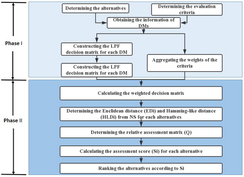
In summary, the procedure of the proposed method is given in Figure 1.

Figure 1. The procedure of the proposed LPFN-CODAS method. Source: Designed by the authors.

5. A case study

The increasing complexity of business environment and emergence of new business models based on new types of information require complex approach towards performance assessment (Iqbal, Chu, & Hali, 2019; Rondovic et al., 2018; Knezevic, 2018; Pan et al., 2019). The proposed decision framework outlined in Section 4 is applied to the case of selecting financial strategies in a multinational firm that involves multiple criteria and DMs (Garg, 2018). The application of the P.F.L.N.s is relevant in this case as the D.M.s may not be experienced enough to respect the constraints associated with I.F.S.s. In addition, the use of linguistic information allows one to assess different alternatives (i.e., investment strategies) that can only be defined in approximate terms due to inherent uncertainties and complexity. Thus, this case study of selecting financial strategies allows the experts to exploit both quantitative and qualitative assessment information to find a best solution.

Assume that a company is about to choose a proper investment strategy at different geographical locations. Specifically, it considers expanding its operations to Asia, Africa or Northern America (these alternatives are denoted by $\{A_1,A_2,A_3\}$). In addition, simultaneous expansion to all the three regions is included in the analysis as A₄. An expert group is established to identify the most promising investment strategy.

The alternatives under consideration are evaluated with respect to the four criteria representing the prospect in the short, medium and long run (denoted as $\{C_1,C_2,C_3\}$) along with the risk profile attached to the alternatives (criterion C₄). Obviously, the first three criteria are benefit ones as the company seeks to enhance the prospect of the investment, whereas the fourth criterion is a cost one as the company seeks to minimise the risk associated with the alternatives. Furthermore, the differences in the importance of the benefit criteria exist as the discount rate affects the preferences of the D.M.s with respect to $\{C_1,C_2,C_3\}.$ Thus, the identification of the investment strategy constitutes an M.C.G.D.M. problem.

The expert group comprises three D.M.s. Due to differences in their background, the experts taking part in the M.C.G.D.M. are assigned with different importance as reflected in the weight vector $({\delta }_1,{\delta }_2,{\delta }_3)=(0.243,0.514,0.243).$ The experts are denoted as $\{D_1,D_2,D_3\}.$ The decision-making proceeds by providing the linguistic ratings from the linguistic term set $S=\{s_0,s_1,s_2,s_3,s_4,s_5,s_6,s_7,s_8\}=\{\text{extremely}\mathrm{}\text{poor},\mathrm{}\text{very}\mathrm{}\text{poor},\mathrm{}\text{poor},\mathrm{}\text{slightly}\mathrm{}\text{poor},\mathrm{}\text{fair},\mathrm{}\text{slightly}\mathrm{}\text{good},\mathrm{}\text{good},\mathrm{}\text{very}\text{good},\mathrm{}\text{extremely}\mathrm{}\text{good}\}.$ These terms are applied to assess the performance of the alternatives with regards to the criteria.

5.1. Determination of criteria weights

We assume that the weights of criteria are unknown. Thus, the procedure given in Section 4.1 is applied to derive the weights from pair-wise comparisons between each pair of criteria. Each expert taking part in the M.C.G.D.M. procedure provides his/her assessment on the perceived importance of the criteria in a pairwise manner. The detailed procedure is given as follows:

Step 1. Each expert provides his/her preferences in regard to the importance of a certain criterion $C_i,i=1,2,3,4$ with respect to each of the other three criteria by conducting pair-wise comparisons. The comparison is based on the linguistic labels from $\overline{S}=\left\{s_{\alpha }\right|\alpha \in [0,8]\}.$ The results of pair-wise comparisons are given in Tables 3–5.

Table 3. The pair-wise comparison of the importance of criteria by expert D₁.

Criteria	C1	C2	C3	C4
C1	(s4, s4)	(s6, s6)	(s5, s3)	(s6, s5)
C2	(s6, s6)	(s4, s4)	(s4, s4)	(s6, s2)
C3	(s3, s5)	(s4, s4)	(s4, s4)	(s3, s3)
C4	(s5, s6)	(s2, s6)	(s3, s3)	(s4, s4)

Source: Designed by the authors.

Table 4. The pair-wise comparison of the importance of criteria by expert D₂.

Criteria	C1	C2	C3	C4
C1	(s4, s4)	(s3, s5)	(s7, s3)	(s2, s6)
C2	(s6, s3)	(s4, s4)	(s3, s5)	(s3, s7)
C3	(s3, s7)	(s5, s3)	(s4, s4)	(s1, s5)
C4	(s6, s2)	(s7, s3)	(s5, s1)	(s4, s4)

Source: Designed by the authors.

Table 5. The pair-wise comparison of the importance of criteria by expert D₃.

Criteria	C1	C2	C3	C4
C1	(s4, s4)	(s3, s6)	(s2, s1)	(s3, s5)
C2	(s6, s3)	(s4, s4)	(s3, s5)	(s3, s2)
C3	(s1, s2)	(s5, s3)	(s4, s4)	(s6, s3)
C4	(s5, s3)	(s2, s3)	(s3, s6)	(s4, s4)

Source: Designed by the authors.

Step 2. The results provided by the three experts are aggregated into a single pair-wise comparison matrix N. In order to aggregate the information across the experts, the L.P.F.W.G.A. operator Eq. (4.15) is utilised. The resulting aggregated pair-wise comparison matrix is shown below: $$N=\left(\begin{array}{cccc}(s_{4.0000},s_{4.0000})& (s_{3.5503},s_{5.5499})& (s_{4.7575},s_{2.6748})& (s_{2.8824},s_{5.5774})\\ (s_{6.0000},s_{4.1619})& (s_{4.0000},s_{4.0000})& (s_{3.2172},s_{4.7939})& (s_{3.5504},s_{5.8802})\\ (s_{2.2971},s_{6.1238})& (s_{4.7361},s_{3.2848})& (s_{4.0000},s_{4.0000})& (s_{2.0185},s_{4.2318})\\ (s_{5.4912},s_{3.8970})& (s_{3.8079},s_{4.1619})& (s_{3.9008},s_{3.7346})& (s_{4.0000},s_{4.0000})\end{array}\right).$$

Step 3. The weights of criteria are established on the basis of the variation of the data within matrix N. Therefore, Eqs (4.16)–(4.18) are applied in order to calculate the overall measures of differences: $$\begin{array}{c}{\gamma }_1=(1.3210,1.03666,1.5628,1.4157),\\ {\gamma }_2=(1.1700,1.1700,1.0079,1.4586),\\ {\gamma }_3=(2.1934,1.7476,1.5657,1.3275),\\ {\gamma }_4=(0.7579,0.7584,0.7905,0.7821).\end{array}$$

Step 4. Finally, the measures obtained in Step 3 are further aggregated by means of Eq. (4.19) to derive criteria weights: $w={(w_1,w_2,w_3,w_4)}^T=(0.2659,0.2396,0.3406,0.1539).$

5.2. Ranking the alternatives

The criteria weights determined by pair-wise comparisons in Section 4.1 can be further used to aggregate preference data on alternatives against criteria provided by the experts. In this sub-section, we focus on the multi-criteria assessment of the alternatives following the procedure outlined in Section 4.2. As an outcome, the four investment strategies are assigned with utility scores and ranked accordingly.

The three experts provide their assessments on alternatives $A_1,\dots ,A_4$ with regards to criteria $C_1,\dots ,C_4.$ The linguistic ratings indicate how well a given alternative perform on a certain criterion. The degrees of satisfaction and dissatisfaction are expressed in the nine-point scale with possible hesitancy due to the nature of L.P.F.N.s (i.e., degree of indeterminacy is allowed for). Specifically, the following linguistic term set is used: $S=\{s_0,s_1,s_2,s_3,s_4,s_5,s_6,s_7,s_8\}=\{\text{extremely}\mathrm{}\text{poor},\mathrm{}\text{very}\mathrm{}\text{poor},\mathrm{}\text{poor},\mathrm{}\text{slightly}\mathrm{}\text{poor},\mathrm{}\text{fair},\mathrm{}\text{slightly}\mathrm{}\text{good},\mathrm{}\text{good},\mathrm{}\text{very}\mathrm{}\text{good},\mathrm{}\text{extremely}\mathrm{}\text{good}\}.$

Step 1. The experts provide their ratings for each alternative according to the four criteria in linguistic terms in S. The results are arranged into individual decision matrices $N^{(1)},N^{(2)},N^{(3)}$ in Tables 6–8. The resulting data are further processed by applying an appropriate aggregation operators (the L.P.F.W.G.A. is used here).

Table 6. Decision matrix $N^{(1)}$ provided by expert D₁.

	C1	C2	C3	C4
A1	(s6, s1)	(s3, s1)	(s3, s3)	(s1, s6)
A2	(s3, s4)	(s3, s4)	(s2, s5)	(s2, s4)
A3	(s1, s3)	(s2, s3)	(s3, s2)	(s6, s1)
A4	(s6, s2)	(s4, s3)	(s5, s1)	(s7, s1)

Source: Designed by the authors.

Table 7. Decision matrix $N^{(2)}$ provided by expert D₂.

	C1	C2	C3	C4
A1	(s3, s2)	(s4, s1)	(s3, s4)	(s2, s3)
A2	(s5, s2)	(s2, s1)	(s3, s4)	(s2, s5)
A3	(s2, s3)	(s3, s3)	(s1, s2)	(s3, s3)
A4	(s5, s2)	(s3, s3)	(s5, s2)	(s4, s1)

Source: Designed by the authors.

Table 8. Decision matrix $N^{(3)}$ provided by expert D₃.

	C1	C2	C3	C4
A1	(s3, s3)	(s3, s5)	(s6, s1)	(s2, s6)
A2	(s3, s2)	(s2, s4)	(s2, s1)	(s3, s4)
A3	(s6, s1)	(s2, s5)	(s3, s4)	(s1, s3)
A4	(s5, s1)	(s4, s4)	(s6, s2)	(s5, s2)

Source: Designed by the authors.

Step 2. The ratings provided by the three experts are aggregated into an aggregated decision matrix N. This is accomplished applying the L.P.F.W.G.A. operator Eq. (4.20). The assessment of the investment strategies depends on both benefit and cost criteria. In this case, the data need to be normalised as Eq. (4.21), resulting in the normalised aggregated decision matrix below: $$\widehat{Y}=\left(\begin{array}{cccc}(s_{3.5504},s_{2.1342})& (s_{3.4781},s_{2.8160})& (s_{3.5504},s_{3.3161})& (s_{1.6900},s_{4.9381})\\ (s_{3.9008},s_{2.6771})& (s_{2.2071},s_{2.9664})& (s_{2.4634},s_{3.9044})& (s_{2.2071},s_{4.5672})\\ (s_{2.2071},s_{2.6748})& (s_{2.4634},s_{3.6617})& (s_{1.7056},s_{2.6771})& (s_{2.7185},s_{2.6748})\\ (s_{5.2265},s_{1.8123})& (s_{3.4502},s_{3.2848})& (s_{5.2265},s_{1.8123})& (s_{4.8380},s_{1.3200})\end{array}\right).$$

Step 3. The criteria have different importance based on the expert ratings discussed in Section 5.1. Accordingly, the normalised aggregated decision matrix $\widehat{Y}$ should be further processed to incorporate the criteria weight information. In this case study we apply arithmetic operator for the P.F.L.N.s Eq. (4.22). The resulting weighted decision matrix is given in Table 9. These values will be employed to identify the theoretical worst-performing alternative.

Table 9. The weighted normalised aggregated decision matrix G.

Alternatives	C1	C2	C3	C4
A1	$(s_{1.9042},s_{5.6299})$	$(s_{1.7701},s_{6.2294})$	$(s_{2.1464},s_{5.9268})$	$(s_{0.6694},s_{7.4275})$
A2	$(s_{2.1112},s_{5.9796})$	$(s_{1.0966},s_{6.3075})$	$(s_{1.4612},s_{6.2659})$	$(s_{0.8804},s_{7.3388})$
A3	$(s_{1.1546},s_{5.9783})$	$(s_{1.2286},s_{6.6339})$	$(s_{1.0030},s_{5.5101})$	$(s_{1.0942},s_{6.7587})$
A4	$(s_{2.9671},s_{5.3904})$	$(s_{1.7547},s_{6.4634})$	$(s_{3.3244},s_{4.8245})$	$(s_{2.0810},s_{6.0627})$

Source: Designed by the authors.

Step 4. The C.O.D.A.S. relies on the reference point the worst-performing (negative ideal) alternative, which is defined by the minimum elements of the columns of the weighted matrix G. For this case study, the negative ideal alternative is given by vector $NS={[n{s}_j]}_{1\times 4}.$ By Eq. (4.22), the elements of N.S. are obtained as: $n{s}_1=(s_{1.1546},s_{5.9796}),n{s}_2=(s_{1.0966},s_{6.6339})n{s}_3=(s_{1.0030},s_{6.2659}),n{s}_4=(s_{0.6694},s_{7.4275}),$

Step 5. The distances between the alternatives and the negative ideal solution are measured to identify the deviations from the worst-performing case. These will be used as the relative measures of the performance of the alternatives. The C.O.D.A.S. involves both Euclidean and Hamming-like distances. Accordingly, Eqs (4.24) and (4.26) are utilised to obtain the distances from the negative ideal solution, ED_i and HLD_i, respectively. The data in G are used to obtain the distances given in Table 10.

Table 10. LPF Weighted Euclidean and Hamming-like distances.

	HLD					ED
	C 1	C2	C3	C4		C1	C2	C3	C4
A1	0.0625	0.0561	0.0953	0.0000	A1	0.0663	0.0599	0.1038	0.0000
A2	0.0797	0.0272	0.0382	0.0176	A2	0.0976	0.0333	0.0468	0.0187
A3	0.0001	0.0110	0.0630	0.0558	A3	0.0001	0.0135	0.0771	0.0599
A4	0.1510	0.0548	0.1934	0.1176	A4	0.1634	0.0604	0.2072	0.1417

Source: Designed by the authors.

Step 6. The distances obtained in Step 5 are employed to compare the alternatives against each other (with the negative ideal solution acting as a reference point) like in a pair-wise manner Eq. (4.28). The resulting matrix Q summarises the comparison result. Table 11 presents the results.

Table 11. Relative assessment matrix (Q).

Alternatives	A1	A2	A3	A4	Si	Rank
A1	−0.1635	−0.0787	0.0000	−0.8093	−1.0515	4
A2	0.1291	0.0000	0.1245	0.0895	0.3430	2
A3	0.0000	0.0848	0.1635	−0.6458	−0.3975	3
A4	0.6458	0.7306	0.8093	0.0000	2.1857	1

Source: Designed by the authors.

Step 7. The distances describing the relative performance of the alternative are aggregated to obtain the utility scores for the alternatives. The analysis proceeds by adding up the elements within each row of matrix Q as outlined in Eq. (4.30). The utility scores S_i are obtained. These are reported in the second column from the right in Table 10. A higher value of S_i implies a higher distance from the negative ideal alternative. Therefore, we rank the alternatives in descending order of S_i. As a result, the mixed strategy (simultaneous expansions in Asia, Africa, and Northern America) is the most preferred. The overall ranking is $A_4\succ A_2\succ A_3\succ A_1.$

6. Comparative analysis

The results of M.C.G.D.M. are often sensitive to different aggregation operators. Accordingly, we conduct a comparative analysis to ascertain whether the results obtained by the L.P.F.-C.O.D.A.S. are comparable in the context of other M.C.D.M. techniques. This kind of analysis allows one to draw conclusions on the validity of the proposed approach.

We compare the results from our proposed L.P.F.-C.O.D.A.S. with those obtained F.L.N.s-A.H.P., I.F.S.-A.H.P., L.N.F.-P.W., I.V.F.-W.D.B.A. and I.V.P.F.-Entropy methods. As there have been different variations of the A.H.P. method in the literature, we follow the proposed version by Panchal et al. (2017). We apply the same decision data in Section 5 for this comparative analysis. The results are given in Table 12. Obviously, the best- and worst-ranked alternatives remain the same across the comparative approaches, and the middle two alternatives are also ranked the same in our proposed approach with five of the seven other approaches, suggesting that ranking result by the L.P.F.-C.O.D.A.S. is reliable.

Table 12. Comparison of ranking results with various fuzzy extensions of C.O.D.A.S.

Methodology	Ranking of alternatives	Best alternatives	Worst alternatives
FLNs-AHP	$A_4\succ A_3\succ A_2\succ A_1$	A4	A1
IFS-AHP	$A_4\succ A_3\succ A_2\succ A_1$	A4	A1
LNF-PW	$A_4\succ A_2\succ A_3\succ A_1$	A4	A1
IVF-WDBA	$A_4\succ A_2\succ A_3\succ A_1$	A4	A1
IVNF-TOPSIS	$A_4\succ A_2\succ A_3\succ A_1$	A4	A1
IVPF-Entropy	$A_4\succ A_2\succ A_3\succ A_1$	A4	A1
IVAIF-VIKOR	$A_4\succ A_2\succ A_3\succ A_1$	A4	A1
Proposed approach	$A_4\succ A_2\succ A_3\succ A_1$	A4	A1

Source: Designed by the authors.

The C.O.D.A.S. method applies an additional distance measure, the Hamming-like distance, if two alternatives cannot be distinguished by the Euclidean distance, i.e., the Euclidean distance between these two alternatives does not exceed the threshold parameter ε; see Eq. (4.28)(4.28) $$Q_{ik}=(E{D}_i-E{D}_k)+(\rho (E{D}_i-E{D}_k)\times (HL{D}_i-HL{D}_k))$$(4.28) . As the threshold parameter is given exogenously, it is important to carry out a sensitivity analysis to check if the ranking is affected by the changes in the threshold parameter. In order to proceed with the sensitivity analysis, we select different values of the threshold parameter and repeat the L.P.F.-C.O.D.A.S. procedure. Fifteen values of the threshold parameter in [0.01, 1] are selected for this exercise and ranking result are given in Table 13, and visually displayed in Figure 2.

Figure 2. Ranking results with various values of parameter ε.

Note: Cases 1–15 correspond to the different values of $\epsilon \in [0.01,1.00]$ as shown in Table 13. Source: Designed by the authors.

Table 13. Ranking results with different values of threshold ε.

ε
Alter.	0.01	0.02	0.03	0.04	0.05	0.06	0.07	0.08	0.09	0.10	0.30	0.50	0.70	0.90	1.00
A1	4	4	4	4	4	4	4	4	4	4	4	3	3	3	3
A2	2	2	2	2	2	2	2	2	2	2	2	4	4	4	4
A3	3	3	3	3	3	3	3	3	3	3	3	2	2	2	2
A4	1	1	1	1	1	1	1	1	1	1	1	1	1	1	1

Source: Designed by the authors.

The results in Table 13 and Figure 2 indicate the ranking results by the L.P.F.-C.O.D.A.S. remain the same when the threshold parameter ε ranges from 0.01 to 0.3. For $\epsilon >0.3,$ the most preferred alternative remains the same (A₄), but the ranking results of the other three alternatives become different. This sensitivity analysis indicates that the L.P.F.-C.O.D.A.S. is not so sensitive to the threshold parameter, especially in terms of the most preferred alternative.

7. Conclusion

This article proposes an extension of the C.O.D.A.S. technique for M.C.G.D.M., so-called L.P.F.-C.O.D.A.S. This proposed approach takes the L.P.F. numbers as basic decision input, which allows D.M.s express their ratings more conveniently. Furthermore, the linguistic information is maintained throughout the aggregation process.

A case study of investment strategy selection is implemented to demonstrate the operationality of the C.O.D.A.S. method. A comparative analysis and sensitivity analysis are carried out to check the performance of the proposed method. Results of the comparative analysis suggest that the results obtained by the L.P.F.-C.O.D.A.S. are consistent with the other M.C.G.D.M. methods. Sensitivity analysis confirms that the ranking results of our approach remains the same for a wide range of the threshold parameter values.

Further research can be carried out to apply different distance functions and threshold rules in the decision-making process. Monte Carlo simulations can also be carried out to identify the best performing settings. The proposed method can be applied for solving problems in different domains.

Disclosure statement

No potential conflict of interest was reported by the author(s).

Additional information

Funding

The work is supported by the Social Science in Universities of Key Project of Anhui Province (No. SK2019A0116), the National Natural Science Foundation of China (Nos. 71572040, 2017YYRW07), Kevin W. Li is also grateful for the financial support from a Discovery Grant funded by the Natural Sciences and Engineering Research Council of Canada (NSERC Grant No. RGPIN-2018-05529), the Natural Science in Universities of General Project of Anhui Province (No. TSKJ2017B22).

References

- Aliakbari Nouri, F., Khalili Esbouei, S., & Antucheviciene, J. (2015). A hybrid MCDM approach based on fuzzy ANP and fuzzy TOPSIS for technology selection. Informatica, 26(3), 369–388. doi:10.15388/Informatica.2015.53
- Atanassov, K. T. (1986). Intuitionistic fuzzy sets. Fuzzy Sets and Systems., 20(1), 87–96. doi:10.1016/S0165-0114(86)80034-3
- Beliakov, G., & James, S. (2014). Averaging aggregation functions for preferences expressed as Pythagorean membership grades and fuzzy orthopairs. IEEE International Conference on Fuzzy Systems, 298–305.
- Bolturk, E. (2018). Pythagorean fuzzy CODAS and its application to supplier selection in a manufacturing firm. Journal of Enterprise Information Management, 31(4), 550–564. doi:10.1108/JEIM-01-2018-0020
- Bolturk, E., & Kahraman, C. (2018). Interval-valued intuitionistic fuzzy CODAS method and its application to wave energy facility location selection problem. Journal of Intelligent and Fuzzy Systems, 35(4), 4865–4877. doi:10.3233/JIFS-18979
- Chen, C. T. (2000). Extensions of the TOPSIS for group decision-making under fuzzy environment. Fuzzy Sets and Systems, 114(1), 1–9. doi:10.1016/S0165-0114(97)00377-1
- Deschrijver, G., & Kerre, E. E. (2002). A generalization of operators on intuitionistic fuzzy sets using triangular norms and conorms. Notes on Intuitionistic Fuzzy Sets, 8(1), 19–27.
- Dorokhov, O., Chernov, V., Dorokhova, L., & Streimkis, J. (2018). Multi-Criteria Choice of Alternatives under Fuzzy Information. Transformations in Business & Economics, 17(2), 95–106.
- Fatma, B. Y., & Gökhan, Ö. (2018). Interval-valued Atanassov intuitionistic fuzzy CODAS method for multi-criteria group decision making problems. Group Decision and Negotiation, 28, 433–452.
- Gao, H., Lu, M., & Wei, Y. (2019). Dual hesitant bipolar fuzzy hamacher aggregation operators and their applications to multiple attribute decision making. Journal of Intelligent & Fuzzy Systems, 37(4), 5755–5766. doi:10.3233/JIFS-18266
- Garg, H. (2016). A novel correlation coefficients between Pythagorean fuzzy sets and its applications to decision-making processes. International Journal of Intelligent Systems, 31(12), 1234–1252. doi:10.1002/int.21827
- Garg, H. (2018). Linguistic Pythagorean fuzzy sets and its applications in multi-attribute decision-making process. International Journal of Intelligent Systems, 33(6), 1234–1263.. doi:10.1002/int.21979
- Ghorabaee, M. K., Amiri, M., Zavadskas, E. K., Hooshmand, R., & Antucheviciene, J. (2017). Fuzzy extension of the CODAS method for multi-criteria market segment evaluation. Journal of Business Economics and Management, 18(1), 1–19. doi:10.3846/16111699.2016.1278559
- Herrera, F., & Martínez, L. (2001). A model based on linguistic 2-tuples for dealing with multigranular hierarchical linguistic contexts in multiexpert decision-making. IEEE Transactions on Systems, Man, and Cybernetics, Part B (Cybernetics), 31(2), 227–234.
- Hosseini, S. T., Lale Arefi, S., Bitarafan, M., Abazarlou, S., & Zavadskas, E. K. (2016). Evaluation types of exterior walls to reconstruct Iran earthquake areas (Ahar Heris Varzeqan) by using AHP and fuzzy methods. International Journal of Strategic Property Management, 20(3), 328–340. doi:10.3846/1648715X.2016.1190794
- Iqbal, S., Chu, J. X., & Hali, S. M. (2019). Projecting impact of CPEC on Pakistan’s electric power crisis. Chinese Journal of Population Resources and Environment, 17(4), 310–321. doi:10.1080/10042857.2019.1681879
- Kahraman, C., Onar, S. C., & Oztaysi, B. (2015). Fuzzy multicriteria decision-making: a literature review. International Journal of Computational Intelligence Systems, 8(4), 637–666. doi:10.1080/18756891.2015.1046325
- Ghorabaee, M. K., Zavadskas, E. K., Turskis, Z., & Antucheviciene, J. (2016). A new combinative distance-based assessment (CODAS) method for multi-criteria decision-making. Economic Computation and Economic Cybernetics Studies and Research, 50(3), 25–44.
- Knezevic, D. (2018). Impact of Blockchain Technology Platform in Changing the Financial Sector and Other Industries. Montenegrin Journal of Economics, 14(1), 109–120. doi:10.14254/1800-5845/2018.14-1.8
- Liang, D. C., Xu, Z. S., & Darko, A. P. (2017). Projection model for fusing the information of Pythagorean fuzzy multicriteria group decision making based on geometric Bonferroni mean. International Journal of Intelligent Systems, 32(9), 966–987. doi:10.1002/int.21879
- Liu, N., He, Y., & Xu, Z. (2019). Evaluate Public-Private-Partnership’s advancement using double hierarchy hesitant fuzzy linguistic PROMETHEE with subjective and objective information from stakeholder perspective. Technological and Economic Development of Economy, 25(3), 386–420. doi:10.3846/tede.2019.7588
- Lu, J., Tang, X., Wei, G., Wei, C., & Wei, Y. (2019). Bidirectional project method for dual hesitant Pythagorean fuzzy multiple attribute decision-making and their application to performance assessment of new rural construction. International Journal of Intelligent Systems, 34(8), 1920–1934. doi:10.1002/int.22126
- Pamucar, D., Badi, I., Sanja, K., & Obradović, R. (2018). A novel approach for the selection of power-generation technology using a linguistic Neutrosophic CODAS method: a case study in Libya. Energies, 11(9), 2489–2514. doi:10.3390/en11092489
- Pan, X. F., Pan, X. Y., Song, M. L., Ai, B. W., & Ming, Y. (2019). Blockchain technology and enterprise operational capabilities: An empirical test. International Journal of Information Management, 101946. DOI:. doi:10.1016/j.ijinfomgt.2019.05.002
- Panchal, D., Chatterjee, P., Shukla, R. K., Choudhury, T., Tamosaitiene, J., et al. (2017). Integrated fuzzy AHP-CODAS framework for maintenance decision in urea fertilizer industry. Economic Computation and Economic Cybernetics Studies and Research, 51(3), 179–196.
- Peng, X. D., & Garg, H. (2018). Algorithms for interval-valued fuzzy soft sets in emergency decision making based on WDBA and CODAS with new information measure. Computers and Industrial Engineering, 119, 439–452.
- Peng, X. D., & Li, W. (2019). Algorithms for interval-valued Pythagorean fuzzy sets in emergency decision making based on multi-parametric similarity measures and WDBA. IEEE Access., 7, 7419–7441. doi:10.1109/ACCESS.2018.2890097
- Peng, X., & Selvachandran, G. (2019). Pythagorean fuzzy set: state of the art and future directions. Artificial Intelligence Review, 52(3), 1873–1927.
- Peng, X., & Yang, Y. (2016). Pythagorean fuzzy Choquet integral based MABAC method for multiple attribute group decision making. International Journal of Intelligent Systems, 31(10), 989–1020. doi:10.1002/int.21814
- Pongpimol, S., Badir, Y., Erik, B., & Sukhotu, V. (2020). A multi-criteria assessment of alternative sustainable solid waste management of flexible packaging. Management of Environmental Quality: An International Journal, 31(1), 201–222. doi:10.1108/MEQ-11-2018-0197
- Reformat, M. Z., & Yager, R. R. (2014). Suggesting recommendations using Pythagorean fuzzy sets illustrated using Netflix movie data. Information processing and management of uncertainty in knowledge-based Systems, 546–556 Berlin: Springer.
- Ren, J. Z. (2018). Sustainability prioritization of energy storage technologies for promoting the development of renewable energy: a novel intuitionistic fuzzy combinative distance-based assessment approach. Renewable Energy., 121, 666–676. doi:10.1016/j.renene.2018.01.087
- Ren, P., Xu, Z., & Gou, X. (2016). Pythagorean fuzzy TODIM approach to multi-criteria decision making. Applied Soft Computing, 42, 246–259. doi:10.1016/j.asoc.2015.12.020
- Rondovic, B., Melovic, B., Mitrovic, S., & Ocovaj, S. B. (2018). Determinants of ECRM Adoption and Diffusion-Multistage Analysis in The South-Eastern Europe. Transformations in Business & Economics, 17(3C), 328–346.
- Tang, X., & Wei, G. (2019). Multiple attribute decision-making with dual hesitant Pythagorean fuzzy information. Cognitive Computation, 11(2), 193–211. doi:10.1007/s12559-018-9610-9
- Vinodh, S., Sai Balagi, T. S., & Patil, A. (2016). A hybrid MCDM approach for agile concept selection using fuzzy DEMATEL, fuzzy ANP and fuzzy TOPSIS. The International Journal of Advanced Manufacturing Technology, 83(9-12), 1979–1987. doi:10.1007/s00170-015-7718-6
- Wang, J., Gao, H., & Wei, G. (2019). The generalized Dice similarity measures for Pythagorean fuzzy multiple attribute group decision making. International Journal of Intelligent Systems, 34(6), 1158–1183. doi:10.1002/int.22090
- Wang, T., & Chang, T. (2005). Fuzzy VIKOR as a resolution for multi-criteria group decision-making. In: 11th International Conference on Industrial Engineering and Engineering Management, Shenyang, China, 352–356.
- Wei, G. W. (2019). Pythagorean fuzzy Hamacher power aggregation operators in multiple attribute decision making. Fundamenta Informaticae, 166(1), 57–85. doi:10.3233/FI-2019-1794
- Wu, L., Gao, H., & Wei, C. (2019). VIKOR method for financing risk assessment of rural tourism projects under interval-valued intuitionistic fuzzy environment. Journal of Intelligent & Fuzzy Systems, 37(2), 2001–2008. doi:10.3233/JIFS-179262
- Xu, Z. S. (2004). A method based on linguistic aggregation operators for group decision making under linguistic preference relations. Information Sciences, 166(1-4), 19–30. doi:10.1016/j.ins.2003.10.006
- Yager, R. R. (2013). Pythagorean fuzzy subsets. In: Proceedings Joint IFSA World Congress and NAFIPS Annual Meeting, Edmonton, Canada. Piscataway, NJ, 57–61.
- Yager, R. R. (2016). Properties and applications of Pythagorean fuzzy sets. Imprecision and Uncertainty in Information Representation and Processing, 332, 119–136.
- Yager, R. R. (2014). Pythagorean membership grades in multi-criteria decision making. IEEE Transactions on Fuzzy Systems, 22(4), 958–965. doi:10.1109/TFUZZ.2013.2278989
- Zadeh, L. A. (1965). Fuzzy sets. Information and Control, 8(3), 338–353. doi:10.1016/S0019-9958(65)90241-X
- Zeng, S. Z. (2017). Pythagorean fuzzy multi-attribute group decision making with probabilistic information and OWA approach. International Journal of Intelligent Systems, 32(11), 1136–1150. doi:10.1002/int.21886
- Zhang, X. L., & Xu, Z. S. (2014). Extension of TOPSIS to multi-criteria decision making with Pythagorean fuzzy sets. International Journal of Intelligent Systems, 29(12), 1061–1078. doi:10.1002/int.21676
- Zhou, J. M., Su, W. H., Baležentis, T., & Streimikiene, D. (2018). Multiple criteria group decision-making considering symmetry with regards to the positive and negative ideal solutions via the Pythagorean normal cloud model for application to economic decisions. Symmetry, 10(5), 140–155. doi:10.3390/sym10050140