The level effect and volatility effect of uncertainty shocks in China

Abstract

Previous studies have assumed that the volatility of exogenous shocks is constant, which can only measure the level effects of uncertain shocks. This article introduces the time-varying volatility model into a Dynamic Stochastic General Equilibrium (D.S.G.E.) model and uses the third-order perturbation method to identify and decompose the level and volatility effects of uncertainty shocks. Based on the results of empirical research in China, the effect of volatility shocks is different from that of level shocks: the effect of level shocks is direct and positive, and its impact is larger, while the effect of volatility shocks is indirect and negative, and its impact is smaller. This article also finds that the impact of uncertainty shocks will lead to economic stagnation, inflation, and the stagflation effect.

Keywords:

• uncertainty shocks
• time-varying volatility
• Dynamic Stochastic General Equilibrium (D.S.G.E.) model
• perturbation method
• stagflation effect

JEL CODES:

• B22
• E32
• E37

1. Introduction

China’s economy is in a critical stage of transformation from high-speed growth to high-quality development. Structural problems in its economic operation cannot be ignored (Zhang et al., 2019). According to the report of the 19th National Congress of the Communist Party of China, high-quality development requires prevention and resolution of major risks. Major emergencies are unexpected or unpredictable, which may cause serious human impacts. For example, the 9/11 terrorist attacks, the S.A.R.S. epidemic, the Wenchuan earthquake, the global financial crisis, C.O.V.I.D.-19 in 2019. Exogenous sudden impacts increase market uncertainty, which has an acute impact on macroeconomic operations (Bloom, 2009).

The core content of macroeconomics is to explore the causes of economic fluctuations. Due to the lack of micro-foundation and rational expectations, Keynesian endogenous business cycle theory cannot explain the economic stagnation, and was criticised by Lucas. The actual business cycle theory and the new Keynesian business cycle theory build a dynamic general equilibrium model based on micro-foundations to simulate the macroeconomic effects of exogenous shocks, which has become the standard paradigm of international macroeconomic research. However, both the actual business cycle theory and the Neo-Keynesian business cycle theory assume that exogenous shocks are homogeneous shocks with constant volatility and ignore the heterogeneous shocks of time-varying volatility. Only the level effects of uncertainty shocks are measured, but the fluctuation effects of uncertainty shocks cannot be measured (Jurado et al., 2015).

The volatility effects of uncertainty shocks have attracted the attention of the international academic community in recent years. Bloom (2009), Fernández-Villaverde, Guerrón-Quintana, Rubio-Ramirez, et al. (2011) and other studies have found that unexpected events such as the financial crisis have increased market uncertainty and affected macroeconomic operations. Leduc and Liu (2016) pointed out that the uncertainty of the economic outlook will have negative effects on the macro economy, such as reduced aggregate demand, rising unemployment and deflation. The analysis of Bloom et al. (2012) showed that increased uncertainty will reduce employment, investment and production, and will also reduce the efficiency of resource redistribution and reduce productivity. Bloom (2014) believed that because developing countries are volatile industries in the international division of labour, coupled with factors such as the instability of reform policies, the macroeconomic impact of uncertainty shocks is greater than that of developed countries. Carrière-Swallow and Céspedes (2013) found that compared with developed countries in Europe and the U.S., when emerging economies are affected by exogenous uncertainties, investment and consumption decline to a greater extent, takes longer to recover and will not cause subsequent excessive economic rebound.

China is at a significant stage of comprehensively deepening reform. The structural problems of economic operation are prominent, the contradictions of overcapacity continue to accumulate, financial risks have begun to manifest, the marginal effects of macroeconomic control policies have declined, and the downward pressure on the economy has been greater. These factors have greatly increased the uncertainty of China’s economic development and market expectations, triggered macroeconomic fluctuations, and increased the risk of economic operations. The research on the impact of uncertainty shocks on China’s macroeconomic operations not only has theoretical value, but also has a major role in policy practice.

In contrast to existing research, this article assumes that the fluctuation rate of exogenous shocks is constant, and only the level effect of uncertain shocks can be measured. This article draws on the research ideas of Bloom (2009) and Fernández-Villaverde, Guerrón-Quintana, Rubio-Ramirez, et al. (2011), introduces the time-varying volatility model into a dynamic stochastic general equilibrium (D.S.G.E.) model, and uses the third-order perturbation method to decompose the level and volatility effects of uncertainty effect. This model is used to empirically study the impact of uncertainty shocks on China’s macroeconomic fluctuations based on Chinese data. The results show that volatility shocks have a completely different effect from level shocks: level shocks are direct and positive, and their intensity is large; volatility shocks are indirect and negative, and their intensity is small; the impact of volatility will not only lead to economic stagnation, but also cause inflation and produce a stagflation effect.

The rest of the article is structured as follows: Section 2 is a review of relevant literature; Section 3 introduces model settings and a stochastic volatility model into a D.S.G.E. model; Section 4 introduces a model solving method; Section 5 is the empirical analysis in China; finally, the conclusions are presented in Section 6.

2. Literature review

Sudden uncertainty research aroused academic attention after the S.A.R.S. outbreak in 2003. Especially after the 2008 Wenchuan earthquake and the U.S. financial crisis, research on sudden shocks was put on the agenda. The National Natural Science Foundation of China has continuously implemented the 2009–2013 major research plan of ‘Unconventional Emergency Management Research’, which has greatly promoted the construction of China’s emergency management theoretical system and the development of interdisciplinary disciplines. However, research on sudden shocks in the academic community mainly focused on emergency management in the micro-sphere. It is necessary to study the impact of sudden shocks on macroeconomic operations and their policy responses from a macro perspective (Tang et al., 2009; Tang et al., 2012). But there are few studies in this area. With the development of international macroeconomic theories and econometric models, recent literature has begun to expand into the field of macroeconomics.

The V.A.R. model is based on the statistical nature of the data and has strong flexibility in the parameter structure, which can better fit the quantitative impact of uncertainty shocks on macroeconomic operations. The V.A.R. model, impulse response function, and variance decomposition are widely used in quantitative research on uncertainty shock and macroeconomic operation (Ma, 2010; Liu & Pan, 2012). However, as a dynamic macro-econometric method, the V.A.R. model does not handle ‘rational expectations’ well enough. It lacks effective integration with ‘general equilibrium analysis’, and micro-foundation of macroeconomic operations (Zheng, 2010; Shen et al., 2012). The V.A.R. model also has problems of index exogenous judgement and lag time in actual operations, which makes the research results have great manoeuverability. Therefore, the V.A.R. model fails to solve effectively the micro-foundation of the impact of sudden shocks on macroeconomic operations and its policy response.

The D.S.G.E. model is based on microeconomic theory and derives macroeconomic equations based on the micro behavioural decisions of economic entities. It meticulously characterises long-term economic equilibrium and its short-term adjustment, and sets structural parameters and economic shocks. Detailed description with identification to avoid Lucas critique has gradually become the mainstream model tool for international macroeconomic econometric analysis (Fang & Wang, 2012; Yang & Li, 2011). The D.S.G.E. model theory and applied research on macroeconomic operation and policy choice in domestic academic circles has accumulated a large amount of research literature, many research methods and rich research conclusions. The existing studies using the D.S.G.E. model in China all assume homogeneous shocks with the same volatility, and ignore heterogeneous shocks with time-varying volatility. This means that the previous research only assumes the first-order rectangular form of uncertainty shock, which reflects the level effects, and is suitable for normal economic periods. It ignores the second-order rectangular form, and it is difficult to accurately describe emergency periods and the impact of uncertainty on macroeconomic operations

In 2009, Nicholas Bloom, a young professor of economics at Stanford University in the U.S., published a research paper entitled ‘The impact of Uncertainty Shocks’ in the Journal of Econometrics. For the first time, based on the stochastic dynamic optimisation model, the time-varying second-order moment model is introduced to describe the uncertainty characteristics of the sudden impact, simulate the dynamic behaviour equation of the micro enterprise after the ‘9/11’ emergency, and reflect its impact on macroeconomic operations through the aggregation of micro enterprise variables. It is found that it will lead to a short-term rapid recession and subsequent economic recovery. The research of Bloom (2009) has the micro-foundations of ‘dynamic’, ‘random’ and rational expectations, and has created a structural analysis framework for studying the impact of uncertainty shocks on macroeconomic operations based on micro foundations. The article became a founding work, which quickly attracted the attention of the academic community after its publication, and has been cited thousands of times.

However, Bloom (2009) only used the equations of corporate behaviour; he does not consider the general equilibrium of the equations of behaviour of residents, corporations, and governments, and does not involve discussion of policy responses. Based on the theory of Bloom (2009), a group of scholars have introduced ‘general equilibrium’ including residents, enterprises, and governments to construct a D.S.G.E. model to study the impact of uncertainty shocks on macroeconomic operations (Fernández-Villaverde, Guerrón-Quintana, Rubio-Ramirez, et al. 2011; Bachmann & Moscarini, 2011; Bachmann & Bayer, 2011; Bloom et al., 2012; Basu & Bundick, 2012; Brede, 2013; Leduc & Liu, 2016) and their fiscal and monetary policies (Keen & Pakko, 2011; Born & Peifer, 2011; Fernández-Villaverde, Guerrón-Quintana, Kuester, et al., 2011; Mumtaz & Zanetti, 2013; Davig & Foerster, 2014). Keen and Pakko (2011) incorporated uncertainty shocks into the framework of D.S.G.E., and explored monetary policy choices under sudden shocks of natural disasters. Fernández-Villaverde, Guerrón-Quintana, Rubio-Ramirez, et al. (2011) constructed a small open economy model, using a stochastic fluctuation model to characterise the impact of real interest rate uncertainty, and selected short-term government bond interest rates and national development data from four emerging economies to study the impact of uncertainty in real interest rates on actual macroeconomic variables. Studies have found that the shock of uncertainty in real interest rates increases the risk of holding foreign debt, which in turn leads to adverse movements in marginal utility and a decline in physical capital gains, thereby reducing consumption and investment, ultimately leading to a decline in output and employment. Based on the standard new Keynesian D.S.G.E. model, Fernández-Villaverde, Guerrón-Quintana, Kuester, et al. (2011) studied the impact of fiscal policy uncertainty shocks on macroeconomic operations, and found that its negative impact was equivalent to the impact of the 25-basis-point innovation of the federal funds rate. Born and Peifer (2011) constructed a new Keynes DSGE model with policy uncertainty and technical uncertainty, and studied its economic impact. Bloom et al. (2012) studied the impact of the sudden impact of the U.S. financial crisis in 2007–2009 on macroeconomic operations and its policy effects. Based on the New Keynes D.S.G.E. model, Basu and Bundick (2012) comparatively analysed the quantitative impact of uncertainty shocks on macroeconomics under the assumptions of price elasticity and found price stickiness. Monetary policy can offset the impact of uncertainty shocks on the macroeconomic downturn. Basu and Bundick (2017) used standard general-equilibrium models to study the effects of uncertainty shocks on output. Alessandri and Mumtaz (2019) analysed the impact of the uncertainty shocks on the American financial crisis. Cuaresma et al. (2020) studied the macroeconomic impact of international uncertainty shocks on G7 countries. Gupta et al. (2020) analysed the impact of uncertainty shocks on 50 developed and emerging economies. Gilchrist et al. (2014), Arellano et al. (2012), Bonciani and Van Roye (2013), Cesa-Bianchi and Corugedo (2014), Christiano et al. (2014), etc. considered the banking sector and credit channels to study the magnifying effect of financial friction.

Incorporating uncertainty shock into the research framework of D.S.G.E. model, and studying its impact on macroeconomic operations and policy responses based on micro foundations have been hot topics in the international academic community in recent years. However, most of the studies are aimed at developed countries in Europe and the U.S., and there is no remodelling specifically for the economic characteristics of developing countries such as China. Bloom (2014) believed that the impact of uncertainty on developing countries is more serious than that of developed countries. Carrière-Swallow and Céspedes (2013) found empirically that when emerging economies are hit by uncertainty, it will take longer to recover, and subsequent economies will not rebound too much. This article will explore the impact of uncertainty shocks on China’s macroeconomic operations, as well as level and volatility effects.

3. Modelling

This article learns from and extends the model framework of Andreasen (2012) to construct a standard new Keynesian D.S.G.E. model. Based on Andreasen’s model framework, this article extends the model from two aspects, including capital stock of production function and central bank. Assume that the economy consists of three sectors, namely the household sector, the corporate sector (the corporate sector is divided into final product producers and intermediate product producers) and the central bank.

The value function of the household sector is set as: (1) $$V_t\equiv \{\begin{array}{c}{u}_t+\beta {(E_t[V_{t+1}^{1-\alpha }])}^{\frac{1}{1-\alpha }},u_t\ge 0\\ u_t-\beta {(E_t[-V_{t+1}^{1-\alpha }])}^{\frac{1}{1-\alpha }},u_t\le 0\end{array}$$(1) Where $\beta$ is discount factor and $\beta \in [0,1],\alpha \in R\backslash \left\{1\right\}.$ Utility function is set to: (2) $$u(c_t,n_t)=\frac{{(c_t^{\nu }{(1-n_t)}^{1-\nu })}^{1-\gamma }}{1-\gamma }$$(2)

Among this, $\gamma \in R\backslash \left\{1\right\},$$\nu \in [0,1]$ and $c_t,n_t$ represent consumption supply and labour supply respectively. It can be seen from equations (1)(1) $$V_t\equiv \{\begin{array}{c}{u}_t+\beta {(E_t[V_{t+1}^{1-\alpha }])}^{\frac{1}{1-\alpha }},u_t\ge 0\\ u_t-\beta {(E_t[-V_{t+1}^{1-\alpha }])}^{\frac{1}{1-\alpha }},u_t\le 0\end{array}$$(1) and (2)(2) $$u(c_t,n_t)=\frac{{(c_t^{\nu }{(1-n_t)}^{1-\nu })}^{1-\gamma }}{1-\gamma }$$(2) that the intertemporal substitution elasticity between consumption is $1/(1-\nu (1-\gamma )),$ reference Swanson (2012). The degree of relative risk aversion preference is $\gamma +\alpha (1-\gamma ).$

The budget constraint for the household sector is: (3) $$m_t+b_t+c_t=r_t{b}_{t-1}-{\tau }_t+w_t{n}_t+t{r}_t$$(3) where $c_t$ is household consumption, $m_t$ is real currency balance, $b_t$ is actual bond holdings, ${\tau }_t$ is actual tax, $w_t$ is actual wage, ${\pi }_t$ is inflation rate, $t{r}_t$ is actual one-time transfer payment.

The business sector is divided into final product manufacturers and intermediate product sectors. Suppose final product manufacturers are in a completely competitive market environment, the fully competitive final product manufacturers use a basket of intermediate products $y_t(i)$ to produce the final product. The production function of the final product manufacturer is expressed as: (4) $$y_t={\left(\underset{0}{\overset{1}{\int }}{y}_t{(i)}^{\frac{\eta }{\eta -1}}di\right)}^{\frac{\eta }{\eta -1}}$$(4)

In the above formula, $\eta >1.$ The following can be obtained from equation (4)(4) $$y_t={\left(\underset{0}{\overset{1}{\int }}{y}_t{(i)}^{\frac{\eta }{\eta -1}}di\right)}^{\frac{\eta }{\eta -1}}$$(4) : (5) $$y_t(i)={\left(\frac{p_t(i)}{p_t}\right)}^{-\eta }{y}_t$$(5)

The total price level is $p_t={[{\int }_0^1{p}_t{(i)}^{1-\eta }di]}^{\frac{1}{1-\eta }}.$

Assume that all intermediate product producers are homogeneous, and intermediate product enterprises use capital and labour to produce differentiated final products. Its production function is: (6) $$y_t(i)=a_t{k}_t{(i)}_{}^{\theta }{n}_t{(i)}^{1-\theta }$$(6) where $k_t$ is the physical capital, $n_t(i)$ is the labour services, and $a_t$ is a variable that represents external technology shocks. Intermediate product producers maximise the net present value of their future profits by optimising their use of labour services $n_t(i)$ and physical capital $k_t.$ Calvo (1983) assumes that a single vendor’s pricing decision comes from a specific optimisation problem. This article adopts the setting in Rotemberg (1982). The starting point is the market environment of monopolistic competitors: under the constraint of the future price adjustment frequency, each manufacturer chooses their nominal prices to maximise their profits whenever possible. Therefore, it is assumed that the cost of the secondary price adjustment of the enterprise is controlled by $\xi \ge 0.$ Under resource constraints (5) and (6), the first enterprise obtains the optimal labour service and the use of physical capital. Therefore, it is assumed that the cost of the secondary price adjustment of the enterprise is controlled. Under the constraints of resource constraints formula (5) and (6), the i-th enterprise obtains the optimal labour service $n_t(i)$ and the use of physical capital $k_t$ by solving formula (7) the amount. (7) $$\underset{n(i),p_t(i)}{\max }{E}_t\sum _{j=0}^{\infty }{M}_{t,t+j}{y}_{t+j}(i)-w_{t+j}{n}_{t+j}(i)-\frac{\xi }{2}{(\frac{p_{t+j}(i)}{p_{t+j-1}(i)}\frac{1}{{\pi }_{ss}}-1)}^2{y}_{t+j}$$(7)

Learning from Liu (2008, 2010), Yuan et al. (2011) and Mei and Gong (2011), the central bank adopts price-based monetary policy rules, also known as interest rate rules: (8) $$R_t=R_{ss}{\left(\frac{R_{t-1}}{R_{ss}}\right)}^{{\rho }_R}{\left(\frac{{\pi }_t}{{\pi }_{ss}}\right)}^{{\varphi }_{\pi }}{\left(\frac{y_t}{y_{ss}}\right)}^{{\varphi }_y}\hspace{0.17em}\text{exp}\hspace{0.17em}({\epsilon }_t^R)$$(8)

Where ${\epsilon }_t^R:\mathit{NID}(0,\mathrm{var}({\epsilon }_t^R))$ is exogenous shock of price-based monetary policy, $0<{\rho }_m<1.$${\pi }_t=P_t/P_{t-1}$ is inflation. $R_{ss},$${\pi }_{ss},$$y_{ss}$ respectively represents the interest rate level, inflation, and output level at steady-state.

The factor market and product market must meet the following market clearing conditions: (9) $$\begin{array}{c}{n}_t={\int }_0^1{n}_t(i)di\\ k_t={\int }_0^1{k}_t(i)di\\ y_t=c_t+g_t+i_t\end{array}$$(9)

It is assumed that the technical shock process obeys the first-order autoregressive process. (10) $$\text{ln}\hspace{0.17em}(a_{t+1}/a_{ss})={\rho }_a\hspace{0.17em}\text{ln}\hspace{0.17em}(a_t/a_{ss})+{\epsilon }_{t+1}^a$$(10)

Where ${\epsilon }_t^a:\mathit{NID}(0,{\sigma }_t^{\epsilon })$ represents the first moment impact of technology, which means the horizontal impact of technology ${\sigma }_t^{\epsilon }$ is variance of random disturbance terms ${\epsilon }_t^a$ of technology, it uses the second-order moment shock to represent the volatility shocks of the technology, which captures the volatility process of exogenous random disturbance terms in the model. The model in this article focuses on how to capture the impact on the economy when the level of technological shocks and fluctuations change independently. It is a key technical issue to separate level shocks and volatility shocks. Andreasen (2012) considers that the D.S.G.E. model, including standard stochastic volatility processes, is not suitable because it only includes level shocks and does not include any high-order moment impacts (such as second-order moments, third-order moments, etc.). In this article, referring to the time-varying volatility model of Andreasen (2012), the volatility shocks are introduced into the model by the following form: $$\begin{array}{l}{a}_{t+1}=a_{ss}+{\sigma }_{t+1}{v}_{t+1}\\ v_{t+1}=\rho v_t+{\epsilon }_{v,t+1}\\ {\sigma }_{t+1}=(1-{\rho }_{\sigma }){\sigma }_{ss}+{\rho }_{\sigma }{\sigma }_t+{\epsilon }_{\sigma ,t+1}\end{array}$$

In the above formula, $a_{ss},{\sigma }_{ss}\ge 0,$$\rho ,{\rho }_{\sigma }\in [0,1],$${\epsilon }_{v,t}:II{D}^{+}(E[{\epsilon }_{v,t}],\mathit{Var}[{\epsilon }_{v,t}]).$ The level effects and volatility effects of uncertainty shock can be distinguished independently.

4. Model solving method

Assuming that the economic entities in the model optimise their economic behaviour under their own budget constraints, a differential system is defined by the following form: (11) $$E_{t}f(Y_{t+1},Y_t,X_{t+1},X_t)=0$$(11) where $E_t$ is expected symbol, vector $X_t$ is prerequisite variable with $n_x\times 1$ dimension. Vector $Y_t$ is non-prerequisite variables with $n_y\times 1$ dimension. Define a formula $n=n_x+n_y.$ State variables $X_t$ can be split into $X_t={[X_t^1;X_t^2]}^{\prime }.$Vector$X_t^1$ consists of endogenous prerequisite variables. Vector $X_t^2$ consists of exogenous vector. $X_t^2$ is defined to be subject to the following random process: $$X_{t+1}^2=\Lambda X_t^2+\tilde{\eta }\sigma {\epsilon }_{t+1}$$

In the above formula, the dimensions of the vector $X_t^2$ and the residual ${\epsilon }_{t+1}$ are both $n_{\epsilon }\times 1.$ And ${\epsilon }_{t+1}$ obeys the mean value of zero, the variance or covariance matrix is independent and identically distributed. $\sigma \ge 0$ and the matrix with dimensions of $n_{\epsilon }\times n_{\epsilon }.$ The modulus of all eigenvalues of the $\Lambda$ matrix is less than 1.

4.1 First-order Taylor expansion

The equation is solved as: (12) $$Y_t=g(X_t,\sigma )$$(12) (13) $$X_{t+1}=h(X_t,\sigma )+\eta \sigma {\epsilon }_{t+1}$$(13) where $\eta$ is a matrix with dimension $n_{\chi }\times n_{\epsilon },$ its form is $\eta =\left[\begin{array}{c}\varphi \\ \tilde{\eta }\end{array}\right].$

Substituting equations (12)(12) $$Y_t=g(X_t,\sigma )$$(12) and (13)(13) $$X_{t+1}=h(X_t,\sigma )+\eta \sigma {\epsilon }_{t+1}$$(13) into (11) gives: (14) $$F(X,\sigma )=E_{t}f(g(h(X,\sigma )+\eta \sigma {\epsilon }^{\prime },\sigma ),g(X,\sigma ),h(X,\sigma )+\eta \sigma {\epsilon }^{\prime },X)=0$$(14)

Then the following can be obtained from equation (14)(14) $$F(X,\sigma )=E_{t}f(g(h(X,\sigma )+\eta \sigma {\epsilon }^{\prime },\sigma ),g(X,\sigma ),h(X,\sigma )+\eta \sigma {\epsilon }^{\prime },X)=0$$(14) : (15) $$F_{X^k,{\sigma }^j}(X,\sigma )=0,\forall X,\sigma ,j,k,$$(15) where $F_{X^k,{\sigma }^j}(X,\sigma )=0$ is derivative of function F to X in order of K and the J-order derivative for $\sigma .$

The first-order approximations of g and h near point$(X,\sigma )=(\overline{X},0)$ are: (16) $$\begin{array}{c}g(X,\sigma )=g(\overline{X},0)+g_X(\overline{X},0)(X-\overline{X})+g_{\sigma }(\overline{X},0)\sigma \\ h(X,\sigma )=h(\overline{X},0)+h_X(\overline{X},0)(X-\overline{X})+h_{\sigma }(\overline{X},0)\sigma \end{array}$$(16)

Substituting the above formula into the formula (15) gives: (17) $$\begin{array}{c}{F}_X(\overline{X},0)=0\\ F_{\sigma }(\overline{X},0)=0\end{array}$$(17)

Using the first expression in equation (17)(17) $$\begin{array}{c}{F}_X(\overline{X},0)=0\\ F_{\sigma }(\overline{X},0)=0\end{array}$$(17) , the values of $g_X$ and $h_X$ can be obtained by solving equations (18)(18) $${[F_X(\overline{X},0)]}_j^i={\left[f_{Y^{\prime }}\right]}_{\alpha }^i{\left[g_X\right]}_{\beta }^{\alpha }{\left[h_X\right]}_j^{\beta }+{\left[f_Y\right]}_{\alpha }^i{\left[g_X\right]}_j^{\alpha }+{\left[f_{X^{\prime }}\right]}_{\beta }^i{\left[h_X\right]}_j^{\beta }+{\left[f_X\right]}_j^i=0$$(18) : (18) $${[F_X(\overline{X},0)]}_j^i={\left[f_{Y^{\prime }}\right]}_{\alpha }^i{\left[g_X\right]}_{\beta }^{\alpha }{\left[h_X\right]}_j^{\beta }+{\left[f_Y\right]}_{\alpha }^i{\left[g_X\right]}_j^{\alpha }+{\left[f_{X^{\prime }}\right]}_{\beta }^i{\left[h_X\right]}_j^{\beta }+{\left[f_X\right]}_j^i=0$$(18)

In the above formula, $i=1,\dots ,n;j,\beta =1,\dots ,n_x;\alpha =1,\dots ,n_y$ and $Y^{\prime }$ is the $Y$ value of $t-1.$ Find the partial derivative of the $Y$ ($Y^{\prime }$) of the $t-1$ period in the function $f.$ The partial derivative is a matrix of $n\times n_y.$ But ${[f_{Y^{\prime }}]}_{\alpha }^i$ is the elements of the $i$ row and $\alpha$ column of the coefficient matrix of the equation obtained by the partial derivative.

Similarly, using the second expression in equation (17)(17) $$\begin{array}{c}{F}_X(\overline{X},0)=0\\ F_{\sigma }(\overline{X},0)=0\end{array}$$(17) , the value of $g_{\delta },h_{\delta }$ can be obtained by solving equation (19)(19) $$\begin{array}{l}{[F_{\sigma }(\overline{X},0)]}^i=E_t\{{\left[f_{Y^{\prime }}\right]}_{\alpha }^i{\left[g_X\right]}_{\beta }^{\alpha }{\left[h_{\sigma }\right]}^{\beta }+{\left[f_{Y^{\prime }}\right]}_{\alpha }^i{\left[g_X\right]}_{\beta }^{\alpha }{\left[\eta \right]}_{\varphi }^{\beta }{\left[{\epsilon }^{\prime }\right]}^{\varphi }+{\left[f_{Y^{\prime }}\right]}_{\alpha }^i{\left[g_{\sigma }\right]}^{\alpha }\\ +{\left[f_Y\right]}_{\alpha }^i{\left[g_{\sigma }\right]}^{\alpha }+{\left[f_{X^{\prime }}\right]}_{\beta }^i{\left[h_{\sigma }\right]}^{\beta }+{\left[f_{X^{\prime }}\right]}_{\beta }^i{\left[\eta \right]}_{\varphi }^{\beta }{\left[{\epsilon }^{\prime }\right]}^{\varphi }\}\\ ={\left[f_{Y^{\prime }}\right]}_{\alpha }^i{\left[g_X\right]}_{\beta }^{\alpha }{\left[h_{\sigma }\right]}^{\beta }+{\left[f_{Y^{\prime }}\right]}_{\alpha }^i{\left[g_{\sigma }\right]}^{\alpha }+{\left[f_Y\right]}_{\alpha }^i{\left[g_{\sigma }\right]}^{\alpha }+{\left[f_{X^{\prime }}\right]}_{\beta }^i{\left[h_{\sigma }\right]}^{\beta }\\ =0;\end{array}$$(19) , (19) $$\begin{array}{l}{[F_{\sigma }(\overline{X},0)]}^i=E_t\{{\left[f_{Y^{\prime }}\right]}_{\alpha }^i{\left[g_X\right]}_{\beta }^{\alpha }{\left[h_{\sigma }\right]}^{\beta }+{\left[f_{Y^{\prime }}\right]}_{\alpha }^i{\left[g_X\right]}_{\beta }^{\alpha }{\left[\eta \right]}_{\varphi }^{\beta }{\left[{\epsilon }^{\prime }\right]}^{\varphi }+{\left[f_{Y^{\prime }}\right]}_{\alpha }^i{\left[g_{\sigma }\right]}^{\alpha }\\ +{\left[f_Y\right]}_{\alpha }^i{\left[g_{\sigma }\right]}^{\alpha }+{\left[f_{X^{\prime }}\right]}_{\beta }^i{\left[h_{\sigma }\right]}^{\beta }+{\left[f_{X^{\prime }}\right]}_{\beta }^i{\left[\eta \right]}_{\varphi }^{\beta }{\left[{\epsilon }^{\prime }\right]}^{\varphi }\}\\ ={\left[f_{Y^{\prime }}\right]}_{\alpha }^i{\left[g_X\right]}_{\beta }^{\alpha }{\left[h_{\sigma }\right]}^{\beta }+{\left[f_{Y^{\prime }}\right]}_{\alpha }^i{\left[g_{\sigma }\right]}^{\alpha }+{\left[f_Y\right]}_{\alpha }^i{\left[g_{\sigma }\right]}^{\alpha }+{\left[f_{X^{\prime }}\right]}_{\beta }^i{\left[h_{\sigma }\right]}^{\beta }\\ =0;\end{array}$$(19)

In the above formula, $i=1,\dots ,n;\alpha =1,\dots ,n_Y;\beta =1,\dots ,n_X;\varphi =1,\dots ,n_{\epsilon }.$

4.2. Second-order Taylor expansion

The uncertain D.S.G.E. model, including time-varying volatility, has a complicated structure. Its solution is a topic of concern for economists. At present, the most common solution of the D.S.G.E. model in domestic and foreign academic circles is linear approximation. The first-order Taylor expansion transforms a complex non-linear model into a relatively simple linearised model, which reduces the difficulty of solving. However, Kim et al. (2003) found that in a simple economic system with only two agents, the solution method of linear approximation could obtain a false result impossible in reality, that is, the welfare under closed economy is higher than that under full risk sharing. This is because the linear approximation method ignores the second-order term of the equilibrium welfare function, resulting in inaccurate results. Schmitt-Grohé and Uribe (2004) concluded that the first-order approximation method is not suitable to deal with welfare comparison problems in random situations or policy environments. They gave a complete non-linear D.S.G.E. model of the second-order Taylor expansion mathematical derivation process and Matlab solver.

Based on the first-order approximation, our next step is to obtain a second-order approximation of the functions $g$ and $h$ at the non-random steady-state $X_t=X$ and $\delta =0.$ A second-order approximation of the functions$g$ and $h$ at point $(X,\sigma )=(\overline{X},0)$ can be expressed as: (20-1) $$\begin{array}{c}{[g(X,\sigma )]}^i={[g(\overline{X},0)]}^i+{[g_X(\overline{X},0)]}_a^i{[(X-\overline{X})]}_a+{[g_{\sigma }(\overline{X},0)]}^i\left[\sigma \right]\\ +\frac{1}{2}{[g_{XX}(\overline{X},0)]}_{ab}^i{[(X-\overline{X})]}_a{[(X-\overline{X})]}_b\\ +\frac{1}{2}{[g_{X\sigma }(\overline{X},0)]}_a^i{[(X-\overline{X})]}_a\left[\sigma \right]\\ +\mathrm{ }\mathrm{ }\frac{1}{2}{[g_{\sigma X}(\overline{X},0)]}_a^i{[(X-\overline{X})]}_a\left[\sigma \right]\\ +\frac{1}{2}{[g_{\sigma \sigma }(\overline{X},0)]}^i\left[\sigma \right]\left[\sigma \right]\end{array}$$(20-1) (20-2) $$\begin{array}{c}{[h(X,\sigma )]}^j={[h(\overline{X},0)]}^j+{[h_X(\overline{X},0)]}_a^j{[(X-\overline{X})]}_a+{[h_{\sigma }(\overline{X},0)]}^j\left[\sigma \right]\\ +\frac{1}{2}{[h_{XX}(\overline{X},0)]}_{ab}^j{[(X-\overline{X})]}_a{[(X-\overline{X})]}_b\\ +\frac{1}{2}{[h_{X\sigma }(\overline{X},0)]}_a^j{[(X-\overline{X})]}_a\left[\sigma \right]\\ +\frac{1}{2}{[h_{\sigma X}(\overline{X},0)]}_a^j{[(X-\overline{X})]}_a\left[\sigma \right]\\ +\frac{1}{2}{[h_{\sigma \sigma }(\overline{X},0)]}^j\left[\sigma \right]\left[\sigma \right],\end{array}$$(20-2)

In the above formula, $i=1,\dots ,n_Y,a,b=1,\dots ,n_x,j=1,\dots ,n_x.$ Find the second-order partial derivatives of $X$ and $\sigma$ in function $F(X,\sigma )$ and substitute the steady-state point $(X,\sigma )=(\overline{X},0)$ into the obtained partial derivatives to solve: (21) $$\begin{array}{l}{[F_{XX}(\overline{X},0)]}_{jk}^i=({\left[f_{Y^{\prime }{Y}^{\prime }}\right]}_{\alpha \gamma }^i{\left[g_X\right]}_{\sigma }^{\gamma }{\left[h_X\right]}_k^{\sigma }+{\left[f_{Y^{\prime }Y}\right]}_{\alpha \gamma }^i{\left[g_X\right]}_k^{\gamma })\\ +{\left[f_{Y^{\prime }{X}^{\prime }}\right]}_{\alpha \gamma }^i{\left[h_X\right]}_k^{\sigma }+{\left[f_{Y^{\prime }X}\right]}_{\alpha \gamma }^i{\left[g_X\right]}_{\beta }^{\alpha }{\left[h_X\right]}_j^{\beta }\\ +{\left[f_{Y^{\prime }}\right]}_{\alpha }^i{\left[g_{XX}\right]}_{\beta \sigma }^{\alpha }{\left[h_X\right]}_k^{\sigma }{\left[h_X\right]}_j^{\beta }\\ +{\left[f_{Y^{\prime }}\right]}_{\alpha }^i{\left[g_X\right]}_{\beta }^{\alpha }{\left[h_{XX}\right]}_{jk}^{\beta }\\ +{\left[f_{Y{Y}^{\prime }}\right]}_{\alpha \gamma }^i{\left[g_X\right]}_{\sigma }^{\gamma }{\left[h_X\right]}_k^{\sigma }+{\left[f_{YY}\right]}_{\alpha \gamma }^i{\left[g_X\right]}_k^{\gamma }\\ +{\left[f_{Y{X}^{\prime }}\right]}_{\alpha \sigma }^i{\left[h_X\right]}_k^{\sigma }+{\left[f_{YX}\right]}_{\alpha \gamma }^i{\left[g_X\right]}_j^{\alpha }\\ +{\left[f_Y\right]}_{\alpha }^i{\left[g_{XX}\right]}_{jk}^{\alpha }+{\left[f_{X^{\prime }{Y}^{\prime }}\right]}_{\beta \gamma }^i{\left[g_X\right]}_{\sigma }^{\gamma }{\left[h_X\right]}_k^{\sigma }\\ +{\left[f_{X^{\prime }Y}\right]}_{\beta \gamma }^i{\left[g_X\right]}_k^{\gamma }+{\left[f_{X^{\prime }{X}^{\prime }}\right]}_{\beta \sigma }^i{\left[h_X\right]}_k^{\sigma }\\ +{\left[f_{X^{\prime }X}\right]}_{\beta k}^i{\left[h_X\right]}_j^{\beta }+{\left[f_{X^{\prime }}\right]}_{\beta }^i{\left[h_{XX}\right]}_{jk}^{\beta }+{\left[f_{X{Y}^{\prime }}\right]}_{j\gamma }^i{\left[g_X\right]}_{\sigma }^{\gamma }{\left[h_X\right]}_k^{\sigma }\\ +{\left[f_{XY}\right]}_{j\gamma }^i{\left[g_X\right]}_k^{\gamma }+{\left[f_{X{X}^{\prime }}\right]}_{j\sigma }^i{\left[h_X\right]}_k^{\sigma }+{\left[f_{XX}\right]}_{jk}^i\\ =0;i=1,\dots ,n;j,k,\beta ,\sigma =1,\dots ,n_X;\alpha ,\gamma =1,\dots ,n_Y\end{array}$$(21)

Similarly, the value of the unknown parameters $g_{\sigma \sigma }$ and $h_{\sigma \sigma }$ can be obtained by solving the linear equation system $F_{\sigma \sigma }(\overline{X},0)=0.$ (22) $$\begin{array}{l}{[F_{\sigma \sigma }(\overline{X},0)]}^i={\left[f_{Y^{\prime }}\right]}_{\alpha }^i{\left[g_X\right]}_{\beta }^{\alpha }{\left[h_{\sigma \sigma }\right]}^{\beta }\\ +{\left[f_{Y^{\prime }{Y}^{\prime }}\right]}_{\alpha \gamma }^i{\left[g_X\right]}_{\sigma }^{\gamma }{\left[\eta \right]}_{\xi }^{\sigma }{\left[g_X\right]}_{\beta }^{\alpha }{\left[\eta \right]}_{\varphi }^{\beta }{\left[I\right]}_{\xi }^{\varphi }\\ +{\left[f_{Y^{\prime }{X}^{\prime }}\right]}_{\alpha \sigma }^i{\left[\eta \right]}_{\xi }^{\sigma }{\left[g_X\right]}_{\beta }^{\alpha }{\left[\eta \right]}_{\varphi }^{\beta }{\left[I\right]}_{\xi }^{\varphi }\\ +{\left[f_{Y^{\prime }}\right]}_{\alpha }^i{\left[g_{XX}\right]}_{\beta \sigma }^{\alpha }{\left[\eta \right]}_{\xi }^{\sigma }{\left[\eta \right]}_{\varphi }^{\beta }{\left[I\right]}_{\xi }^{\varphi }\\ +{\left[f_{Y^{\prime }}\right]}_{\alpha }^i{\left[g_{\sigma \sigma }\right]}^{\alpha }+{\left[f_Y\right]}_{\alpha }^i{\left[g_{\sigma \sigma }\right]}^{\alpha }+{\left[f_{X^{\prime }}\right]}_{\beta }^i{\left[h_{\sigma \sigma }\right]}^{\beta }\\ +{\left[f_{X^{\prime }{Y}^{\prime }}\right]}_{\beta \gamma }^i{\left[g_X\right]}_{\sigma }^{\gamma }{\left[\eta \right]}_{\xi }^{\sigma }{\left[\eta \right]}_{\varphi }^{\beta }{\left[I\right]}_{\xi }^{\varphi }\\ +{\left[f_{X^{\prime }{X}^{\prime }}\right]}_{\beta \sigma }^i{\left[\eta \right]}_{\xi }^{\sigma }{\left[\eta \right]}_{\varphi }^{\beta }{\left[I\right]}_{\xi }^{\varphi }\\ =0;\\ i=1,\dots ,n;\alpha ,\gamma =1,\dots ,n_Y;\beta ,\sigma =1,\dots ,n_X;\varphi ,\xi =1,\dots ,n_{\epsilon }.\end{array}$$(22)

The value of $g_{X\sigma }$ and $h_{X\sigma }$ at the steady-state value $(\overline{X},0)$ is equal to zero, $g_{\sigma }=0,$$h_{\sigma }=0$ and all terms in the equation that include $g_{\sigma }$ or $h_{\sigma }$ are zero, so that the function $F_{\sigma X}(\overline{X},0)=0$ can be written as follows: (23) $$\begin{array}{c}{[F_{\sigma X}(\overline{X},0)]}_j^i={\left[f_{Y^{\prime }}\right]}_{\alpha }^i{\left[g_X\right]}_{\beta }^{\alpha }{\left[h_{\sigma X}\right]}_j^{\beta }+{\left[f_{Y^{\prime }}\right]}_{\alpha }^i{\left[g_{\sigma X}\right]}_{\gamma }^{\alpha }{\left[h_X\right]}_j^{\beta }+{\left[f_Y\right]}_{\alpha }^i{\left[g_{\sigma X}\right]}_j^{\alpha }\\ +{\left[f_{X^{\prime }}\right]}_{\beta }^i{\left[h_{\sigma X}\right]}_j^{\beta }=0;\end{array}$$(23)

In the above formula, $i=1,\dots ,n;\alpha =1,\dots ,n_Y;\beta ,\gamma ,j=1,\dots ,n_X.$

Equation (23)(23) $$\begin{array}{c}{[F_{\sigma X}(\overline{X},0)]}_j^i={\left[f_{Y^{\prime }}\right]}_{\alpha }^i{\left[g_X\right]}_{\beta }^{\alpha }{\left[h_{\sigma X}\right]}_j^{\beta }+{\left[f_{Y^{\prime }}\right]}_{\alpha }^i{\left[g_{\sigma X}\right]}_{\gamma }^{\alpha }{\left[h_X\right]}_j^{\beta }+{\left[f_Y\right]}_{\alpha }^i{\left[g_{\sigma X}\right]}_j^{\alpha }\\ +{\left[f_{X^{\prime }}\right]}_{\beta }^i{\left[h_{\sigma X}\right]}_j^{\beta }=0;\end{array}$$(23) is a system of linear equations with $n\times n_X$ dimensions. The $n\times n_X$ unknown parameters contained in the system of equations can be obtained from $g_{\sigma X}$ and $h_{\sigma X}$ at steady-state values. It is clear that the unknown parameters of this equations system are homogeneous, so if the only solution exists, then there will be: (24) $$\begin{array}{c}{g}_{\sigma X}=0\\ h_{\sigma X}=0\end{array}$$(24)

The above formula shows that in the second-order approximation, the coefficients of the linear part of the state vector in the policy function do not depend on the magnitude of the related shock of the variance, that is, the coefficients of the equation in the policy function are independent of the shock of the fluctuation.

4.3. Third-order perturbation

The research by Fernández-Villaverde, Guerrón-Quintana, Rubio-Ramirez, et al. (2011) found that according to the model’s Certainty Equivalent principle, the first-order linear approximation of the D.S.G.E. model, the policy response function depends only on the level shocks of the first-order moment, and the volatility shocks of the second-order moment are not reflected in the strategy function, or the influence coefficient of these variables is zero, so it is impossible to capture the impact of random fluctuations on the macroeconomic system. The second-order approximation of the D.S.G.E. model does not separate level shocks and volatility shocks separately, and only indirectly captures the combined effects of level shocks and volatility shocks through the cross-product term. When level shocks are zero, volatility shocks have no effect on other variables. In order to be able to study the macroeconomic impact of random volatility shocks independently, Fernández-Villaverde, Guerrón-Quintana, Rubio-Ramirez, et al. (2011) proposed the use of third-order perturbation methods to solve D.S.G.E. models containing random fluctuations. The third-order approximation of the D.S.G.E. model can introduce random fluctuation shock as an independent variable into the corresponding function of the policy, and its coefficient is not zero. Scholars such as Fernández-Villaverde, Guerrón-Quintana, Kuester, et al. (2011), Born and Peifer (2011), Andreasen (2012) and Basu and Bundick (2012) all used the third-order perturbation method to solve D.S.G.E. models containing random fluctuations. Fernández-Villaverde, Guerrón-Quintana, Rubio-Ramirez, et al. (2011) used higher-order estimates to find that the cubic terms of the corresponding function of the policy are significant, but higher-order numbers such as fourth-order, fifth-order, and sixth-order have little effect.

The third-order approximation of the function $g,h$ at the steady-state value $(X,\sigma )=(\overline{X},0)$ is: (25-1) $$\begin{array}{l}{[g(X,\sigma )]}^{{\beta }_1}=g(\overline{X},0)+{[g_X(\overline{X},0)]}_{{\alpha }_1}^{{\beta }_1}{[(X-\overline{X})]}^{{\alpha }_1}\\ +\frac{1}{2}{[g_{XX}(\overline{X},0)]}_{{\alpha }_1{\alpha }_2}^{{\beta }_1}{[(X-\overline{X})]}^{{\alpha }_1}{[(X-\overline{X})]}^{{\alpha }_2}\\ +\frac{1}{2}{[g_{\sigma \sigma }(\overline{X},0)]}^{{\beta }_1}\left[\sigma \right]\left[\sigma \right]\\ +\frac{1}{6}{[g_{\mathit{XXX}}(\overline{X},0)]}_{{\alpha }_1{\alpha }_2{\alpha }_3}^{{\beta }_1}{[(X-\overline{X})]}^{{\alpha }_1}{[(X-\overline{X})]}^{{\alpha }_2}{[(X-\overline{X})]}^{{\alpha }_3}\\ +\frac{3}{6}{[g_{\sigma \sigma X}(\overline{X},0)]}_{{\alpha }_3}^{{\beta }_1}\left[\sigma \right]\left[\sigma \right]{[(X-\overline{X})]}^{{\alpha }_3}\\ +\frac{3}{6}{[g_{\sigma XX}(\overline{X},0)]}_{{\alpha }_2{\alpha }_3}^{{\beta }_1}\left[\sigma \right]{[(X-\overline{X})]}^{{\alpha }_2}{[(X-\overline{X})]}^{{\alpha }_3}\\ +\frac{1}{6}{[g_{\sigma \sigma \sigma }(\overline{X},0)]}^{{\beta }_1}\left[\sigma \right]\left[\sigma \right]\left[\sigma \right]\end{array}$$(25-1) (25-2) $$\begin{array}{l}{[h(X,\sigma )]}^{{\beta }_1}=h(\overline{X},0)+{[h_X(\overline{X},0)]}_{{\alpha }_1}^{{\gamma }_1}{[(X-\overline{X})]}^{{\alpha }_1}\\ +\frac{1}{2}{[h_{XX}(\overline{X},0)]}_{{\alpha }_1{\alpha }_2}^{{\gamma }_1}{[(X-\overline{X})]}^{{\alpha }_1}{[(X-\overline{X})]}^{{\alpha }_2}\\ +\frac{1}{2}{[h_{\sigma \sigma }(\overline{X},0)]}^{{\gamma }_1}\left[\sigma \right]\left[\sigma \right]\\ +\frac{1}{6}{[h_{\mathit{XXX}}(\overline{X},0)]}_{{\alpha }_1{\alpha }_2{\alpha }_3}^{{\gamma }_1}{[(X-\overline{X})]}^{{\alpha }_1}{[(X-\overline{X})]}^{{\alpha }_2}{[(X-\overline{X})]}^{{\alpha }_3}\\ +\frac{3}{6}{[h_{\sigma \sigma X}(\overline{X},0)]}_{{\alpha }_3}^{{\gamma }_1}\left[\sigma \right]\left[\sigma \right]{[(X-\overline{X})]}^{{\alpha }_3}\\ +\frac{3}{6}{[h_{\sigma XX}(\overline{X},0)]}_{{\alpha }_2{\alpha }_3}^{{\gamma }_1}\left[\sigma \right]{[(X-\overline{X})]}^{{\alpha }_2}{[(X-\overline{X})]}^{{\alpha }_3}\\ +\frac{1}{6}{[h_{\sigma \sigma \sigma }(\overline{X},0)]}^{{\gamma }_1}\left[\sigma \right]\left[\sigma \right]\left[\sigma \right]\end{array}$$(25-2)

In the above formula, ${\beta }_1=1,\dots ,n_Y;{\gamma }_1=1,\dots ,n_X;{\alpha }_1,{\alpha }_2,{\alpha }_3=1,\dots ,n_X.$ By making the derivative of the function $F(X,\sigma )$ equal to 0, we can solve the values of unknown parameters contained in the linear system after the third-order approximate expansion. Drawing on the processing method of Judd and Guu (1997), the solution process can actually be simplified to find only the solution of a linear system, which simplifies the calculation process and reduces the calculation difficulty.

First, it can be seen that: (26) $$\begin{array}{l}{[F_{\mathit{XXX}}(\overline{X},0)]}_{{\alpha }_1{\alpha }_2{\alpha }_3}^i={\left[f_{Y^{\prime }}\right]}_{{\beta }_1}^i{\left[g_{\mathit{XXX}}\right]}_{{\gamma }_1{\gamma }_2{\gamma }_3}^{{\beta }_1}{\left[h_X\right]}_{{\alpha }_3}^{{\gamma }_3}{\left[h_X\right]}_{{\alpha }_2}^{{\gamma }_2}{\left[h_X\right]}_{{\alpha }_1}^{{\gamma }_1}\\ +{\left[f_{Y^{\prime }}\right]}_{{\beta }_1}^i{\left[g_X\right]}_{{\gamma }_1}^{{\beta }_1}{\left[h_{\mathit{XXX}}\right]}_{{\alpha }_1{\alpha }_2{\alpha }_3}^{{\gamma }_1}\\ +{\left[f_Y\right]}_{{\beta }_1}^i{\left[g_{\mathit{XXX}}\right]}_{{\alpha }_1{\alpha }_2{\alpha }_3}^{{\beta }_1}+{\left[f_{X^{\prime }}\right]}_{{\gamma }_1}^i{\left[h_{\mathit{XXX}}\right]}_{{\alpha }_1{\alpha }_2{\alpha }_3}^{{\gamma }_1}\\ +{\left[b^1\right]}_{{\alpha }_1{\alpha }_2{\alpha }_3}^i\\ =0\end{array}$$(26)

In the above formula, $i=1,\dots ,n;{\alpha }_1,{\alpha }_2,{\alpha }_3=1,\dots n_X.$ The value of ${[b^1]}_{{\alpha }_1{\alpha }_2{\alpha }_3}^i$ depends on the value of $g_X,h_X,g_{XX},h_{XX}$ in the first, second, and third derivatives of function $f.$ Please refer to the specific derivation process (Andreasen, 2012). This article considers ${[b^1]}_{{\alpha }_1{\alpha }_2{\alpha }_3}^i$ as a known non-zero value. Solving the non-zero matrix $g_{\mathit{XXX}},h_{\mathit{XXX}}$ can obtain: (27) $$\begin{array}{l}{[F_{\sigma \sigma X}(\overline{X},0)]}_{{\alpha }_3}^i={\left[f_{Y^{\prime }}\right]}_{{\beta }_1}^i{\left[g_X\right]}_{{\gamma }_1}^{{\beta }_1}{\left[h_{\sigma \sigma X}\right]}_{{\alpha }_3}^{{\gamma }_3}+{\left[f_Y\right]}_{{\beta }_1}^i{\left[g_{\sigma \sigma X}\right]}_{{\gamma }_3}^{{\beta }_1}{\left[h_X\right]}_{{\alpha }_3}^{{\gamma }_3}\\ +{\left[f_Y\right]}_{{\beta }_1}^i{\left[g_{\sigma \sigma X}\right]}_{{\alpha }_3}^{{\beta }_1}+{\left[f_{X^{\prime }}\right]}_{{\gamma }_1}^i{\left[h_{\sigma \sigma X}\right]}_{{\alpha }_3}^{{\gamma }_1}+{\left[b^2\right]}_{{\alpha }_3}^i\\ =0\end{array}$$(27)

In the above formula, $i=1,\dots ,n;{\alpha }_3=1,\dots n_X;$ and ${[b^2]}_{{\alpha }_3}^i$ is also a known non-zero value; $g_{\sigma XX}、h_{\sigma XX}$ value can be obtained by the following system: (28) $$\begin{array}{l}{[F_{\sigma XX}(\overline{X},0)]}_{{\alpha }_2{\alpha }_3}^i={\left[f_{Y^{\prime }}\right]}_{{\beta }_1}^i{\left[g_X\right]}_{{\gamma }_1}^{{\beta }_1}{\left[h_{\sigma XX}\right]}_{{\alpha }_2{\alpha }_3}^{{\gamma }_1}+{\left[f_{Y^{\prime }}\right]}_{{\beta }_1}^i{\left[g_{\sigma XX}\right]}_{{\gamma }_2{\gamma }_3}^{{\beta }_1}{\left[h_X\right]}_{{\alpha }_3}^{{\gamma }_3}{\left[h_X\right]}_{{\alpha }_2}^{{\gamma }_2}\\ +{\left[f_Y\right]}_{{\beta }_1}^i{\left[g_{\sigma XX}\right]}_{{\alpha }_2{\alpha }_3}^{{\beta }_1}+{\left[f_{X^{\prime }}\right]}_{{\gamma }_1}^i{\left[h_{\sigma XX}\right]}_{{\alpha }_2{\alpha }_3}^{{\gamma }_1}\\ =0\end{array}$$(28)

In the above formula, $i=1,2,\dots ,n⏧$ ${\alpha }_2,{\alpha }_3=1,2,\dots ,n_X;$ $g_{\sigma XX}=0、h_{\sigma XX}=0⏧$ the value of $g_{\sigma \sigma \sigma }、h_{\sigma \sigma \sigma }$ can be obtained by the formula (29): (29) $$\begin{array}{l}{[F_{\sigma \sigma \sigma }(\overline{X},0)]}^i=({\left[f_{Y^{\prime }}\right]}_{{\beta }_1}^i+{\left[f_Y\right]}_{{\beta }_1}^i){\left[g_{\sigma \sigma \sigma }\right]}^{{\beta }_1}+({\left[f_{Y^{\prime }}\right]}_{{\beta }_1}^i{\left[g_X\right]}_{{\gamma }_1}^{{\beta }_1}+{\left[f_Y\right]}_{{\beta }_1}^i){\left[h_{\sigma \sigma \sigma }\right]}^{{\gamma }_1}\\ +{\left[b^3\right]}^i\\ =0\end{array}$$(29)

Among this, $i=1,2,\dots ,n.$ The symmetry of the random perturbation distribution has an important effect on linear systems (29). If all the disturbance terms are distributed symmetrically, then all third-order moments are 0, ${[b^3]}^i=0.$ In this case, the linear system (29) is homogeneous, $g_{\sigma \sigma \sigma }=0、h_{\sigma \sigma \sigma }=0;$ If some perturbations in the linear system (22) are asymmetrically distributed, then${[b^3]}^i\ne 0,$ $g_{\sigma \sigma \sigma }$ and $h_{\sigma \sigma \sigma }$ are not 0 in this case. This article sets the random perturbations included in the model as an asymmetric distribution so $g_{\sigma \sigma \sigma }\ne 0$ and $h_{\sigma \sigma \sigma }\ne 0.$

The above is the derivation process of the third-order Taylor approximation expansion. The third-order Taylor approximation of the equations in the model can separate level shocks and volatility shocks separately, so that the impact of volatility shocks on the economy can be studied separately.

4.4. Solution results

Functions$g$ and$h$ find the second derivative of different variables $({\mathrm{X}}_{\mathrm{t}}^1,{\mathrm{Z}}_{\mathrm{t}-1},{\hspace{0.17em}\text{log}\hspace{0.17em}\mathrm{\sigma }}_{\mathrm{t}-1},{\mathrm{\epsilon }}_{\mathrm{t}},{\mathrm{u}}_{\mathrm{t}}).$ The results are shown in Table 1.

Table 1. Second derivative.

${\mathrm{X}}_{\mathrm{t}}^1{\mathrm{X}}_{\mathrm{t}}^1\ne 0$	${\mathrm{X}}_{\mathrm{t}}^1{\mathrm{Z}}_{\mathrm{t}-1}\ne 0$	${\mathrm{X}}_{\mathrm{t}}^1{\mathrm{ }\hspace{0.17em}\text{log}\hspace{0.17em}\mathrm{\sigma }}_{\mathrm{t}-1}=0$	${\mathrm{X}}_{\mathrm{t}}^1{\mathrm{\epsilon }}_{\mathrm{t}}\ne 0$	${\mathrm{X}}_{\mathrm{t}}^1{\mathrm{u}}_{\mathrm{t}}=0$	${\mathrm{X}}_{\mathrm{t}}^1\mathrm{\sigma }=0$
	${\mathrm{Z}}_{\mathrm{t}-1}{\mathrm{Z}}_{\mathrm{t}-1}\ne 0$	${\mathrm{Z}}_{\mathrm{t}-1}{\hspace{0.17em}\text{log}\hspace{0.17em}\mathrm{\sigma }}_{\mathrm{t}-1}=0$	${\mathrm{Z}}_{\mathrm{t}-1}{\mathrm{\epsilon }}_{\mathrm{t}}\ne 0$	${\mathrm{Z}}_{\mathrm{t}-1}{\mathrm{u}}_{\mathrm{t}}=0$	${\mathrm{Z}}_{\mathrm{t}-1}\mathrm{\sigma }=0$
		${\hspace{0.17em}\text{log}\hspace{0.17em}\mathrm{\sigma }}_{\mathrm{t}-1}{\hspace{0.17em}\text{log}\hspace{0.17em}\mathrm{\sigma }}_{\mathrm{t}-1}=0$	${\hspace{0.17em}\text{log}\hspace{0.17em}\mathrm{\sigma }}_{\mathrm{t}-1}{\mathrm{\epsilon }}_{\mathrm{t}}\ne 0*$	${\hspace{0.17em}\text{log}\hspace{0.17em}\mathrm{\sigma }}_{\mathrm{t}-1}{\mathrm{u}}_{\mathrm{t}}=0$	${\hspace{0.17em}\text{log}\hspace{0.17em}\mathrm{\sigma }}_{\mathrm{t}-1}\mathrm{\sigma }=0$
			${\mathrm{\epsilon }}_{\mathrm{t}}{\mathrm{\epsilon }}_{\mathrm{t}}\ne 0$	${\mathrm{\epsilon }}_{\mathrm{t}}{\mathrm{u}}_{\mathrm{t}}\ne 0*$	${\mathrm{\epsilon }}_{\mathrm{t}}\mathrm{\sigma }=0$
				${\mathrm{u}}_{\mathrm{t}}{\mathrm{u}}_{\mathrm{t}}=0$	${\mathrm{u}}_{\mathrm{t}}\mathrm{\sigma }=0$
					$\mathrm{\sigma }\mathrm{\sigma }\ne 0$

Source: The Authors.

It can be seen from Table 1 that the coefficient of volatility shock (${\hspace{0.17em}\text{log}\hspace{0.17em}\mathrm{\sigma }}_{\mathrm{t}-1}$) is not zero only when it is cross-multiplied with the disturbance term of level shocks (${\hspace{0.17em}\text{log}\hspace{0.17em}\mathrm{\sigma }}_{\mathrm{t}-1}{\mathrm{\epsilon }}_{\mathrm{t}}$), and the disturbance term (${\mathrm{u}}_{\mathrm{t}}$) of volatility shock is not zero only when it is cross-multiplied with the perturbation term of level shocks (${\mathrm{\epsilon }}_{\mathrm{t}}{\mathrm{u}}_{\mathrm{t}}$), so the second-order approximation can only be captured indirectly through the cross-terms of level shocks and volatility shocks, and they cannot be separated.

Define $s_t^i$ as the i-th variable in$s_t$ vector. Since $s_t$ have n variables except perturbation parameters, so$i=1,2,\dots \mathrm{n}.$ It can be concluded that the third-order perturbation is an approximation of the endogenous state vector. Take the endogenous state variable consumption as an example: $${\stackrel{⌢}{c}}_t\approx {\psi }_i^k{s}_t^i+\frac{1}{2}{\psi }_{i,j}^k{s}_t^i{s}_t^j+\frac{1}{6}{\psi }_{i,j,l}^k{s}_t^i{s}_t^j{s}_t^l$$ ${\psi }_{i,..}^k$ is a scalar, there is the following tensor representation: $${\psi }_i^k{s}_t^i=\sum _{i=1}^n{\psi }_i^k{s}_t^i,{\psi }_{i,j}^k{s}_t^i{s}_t^j=\sum _{i=1}^n\sum _{j=1}^n{\psi }_{i,j}^k{s}_t^i{s}_t^j,{\psi }_{i,j,l}^k{s}_t^i{s}_t^j{s}_t^l=\sum _{i=1}^n\sum _{j=1}^n\sum _{l=1}^n{\psi }_{i,j,l}^k{s}_t^i{s}_t^j{s}_t^l$$

Express capital in the above formula without causing misunderstanding. The parameters ${\psi }_i^k、{\psi }_{i,j}^k、{\psi }_{i,j,l}^k$ respectively represent the parameter value of the first, second, and third derivatives of the function $k_{t+1}=k(s_t)$ at the steady-state point.

5. Empirical analysis

5.1. Parameter calibration

The thesis parameters are set by calibration method. With reference to Andreasen (2012), set the values of $\gamma$ and $\nu$ to 2.5 and 0.35 respectively. These two values set the intertemporal substitution elasticity of consumption to 0.66. This intertemporal substitution elasticity value is currently used in most references. This value can be said to be a standard value in the D.S.G.E. model. $\beta$ is the discount factor. Refer to Liu (2010) and Zhang (2012) to set it to 0.99. $\xi$ is the coefficient of the quadratic price adjustment cost function of the investment. Set it to 260 with reference to Andreasen (2012). At present, the use of the D.S.G.E. model in China to study economic problems is generally based on the logarithmic linearised equations. The median value of the linearised equation is 0.75, which is close to the estimates of Yuan et al. (2011). $\delta$ is the capital depreciation rate. With reference to Mei and Gong (2011), Li et al. (2010) set the annual depreciation rate to 0.1. $\theta$ is the proportion of labour force in the production function of the enterprise. Its value is set to 0.387 by referring to Yuan et al. (2011). $\eta$ is the mutual substitution elasticity of intermediate products, and its value is set to 6 with reference to Andreasen (2012) in this article. Refer to Liu (2010) for the steady-state value of model variable, and set the steady-state value of labour supply as$n=1/3.$ Set the steady-state value $\pi ={(1.04)}^{1/4}\approx 1.01$ of inflation and steady-state value $R_{ss}=1.028$ of $R_{ss}$ similar to the calibration value of Jin et al. (2013). For the first-order autoregressive coefficient ${\rho }_a$ of technological progress, refer to the values obtained by Bayesian estimation by Liu (2008), Jin et al. (2013) and set it to 0.95. For the convenience of calculation, the coefficient ${\rho }_{a\delta }$ of the stochastic volatility process and the steady-state value ${\delta }_{{\delta }_{ss}}$ of the volatility refer to Andreasen (2012) and set it to 0.99 and 0.0075, and the standard deviation of ${\delta }_{ss}$ to 0.00265.

The calibration values of monetary policy parameters in this article mainly come from the values obtained by Liu (2010) through Bayesian estimation and G.M.M. estimates by Ma and Wei (2011). The positive monetary policy parameter calibration values are ${\rho }_r=0.95,{\phi }_{\pi }=1.12,{\phi }_y=0.3$ respectively. The calibration values of the robust monetary policy parameters are ${\rho }_r=0.95,{\phi }_{\pi }=0.9,{\phi }_y=0.3$ respectively (Table 2).

Table 2. Model parameter calibration.

$\gamma$	$\nu$	$\beta$	$\eta$	$\theta$	$\xi$	$\delta$	$n$	${\pi }_{ss}$	${\rho }_a$	${\rho }_g$
2.5	0.35	0.99	6	0.387	260	0.1	1/3	1.01	0.95	0.90
${\rho }_{a\delta }$	${\delta }_{{\delta }_{ss}}$	${\delta }_{ss}$	$R_{ss}$	$u_{ss}$	$a_{ss}$	$g_{ss}/y_{ss}$	$b_{ss}/y_{ss}$	${\tau }_{ss}/y_{ss}$	${\lambda }_b$	${\gamma }_{by}$
0.99	0.0075	0.00265	1.028	1.01	1	0.17	0.13	0.175	0.22	0.16

Source: The Authors.

5.2. Numerical simulation results

Figure 1 reflects the comparison results of level shocks and volatility shocks of the technology. The level shocks of technology are a direct effect, and its performance has a positive impact on the operation of the macro economy: increased output, increased consumption, reduced labour demand, reduced inflation, and increased investment. This is because technological progress has increased the productivity of enterprises. The reduction of labour and capital used in the same output is shown by the negative fluctuation of labour in the figure. This leads to a decline in the actual marginal cost of production, an increase in profit margins, and a profitable expansion of the output of the enterprise. The enterprise will increase investment to expand the scale of output, which is reflected by positive fluctuations in investment and output. Consumption fluctuates downward in the short-term, followed by consumption growth, which shows the fluctuation of consumption first in the figure and then upward. One possible explanation is due to the decline in labour demand in the short term (Liu, 2010). The reduction in the actual marginal cost of production of the enterprise creates downward pressure on the price level of the company’s products, and the decline in product prices creates downward pressure on inflation, which is reflected in the downward fluctuation of inflation in the figure.

Figure 1. Macroeconomic Effects of Level Shocks and Volatility Shocks (Active Monetary Policy). Source: The Authors.

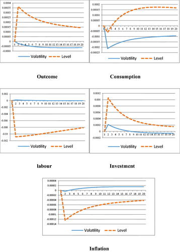
The impact of technological fluctuations is an indirect effect. It exerts a negative impact on the macroeconomic operation by affecting the psychological expectations of economic actors: output decreases, consumption decreases, labour demand increases, inflation rises, and investment increases first and then less. Preventive saving psychology (Born & Peifer, 2011) classifies uncertainty into three categories: the Hartman-Abel effect, option effect, and preventive savings motivation. Basu and Bundick (2012) believe that the increase in uncertainty in the future will lead to an increase in ‘precautionary saving’ and the reduction of people’s current consumption. They also believe that the increase in uncertainty will lead to ‘preventive labour supply’. With the increase of precautionary labour supply, people are willing to provide more labour at the same wage level or still willing to provide the same labour at a lower wage level. Under the shock of fluctuations, future uncertainty increases. Similar research results are obtained in this article, which are shown in Figure 1 as negative fluctuations in consumption and positive fluctuations in labour. The reduction of consumption in the current period reduces the total social demand. In order to reduce the inventory, the enterprise will reduce the output scale, and the output will decline, which will be reflected by the negative fluctuation of output.

Basu and Bundick (2012) concluded that output will not change, consumption will decrease, and investment will show an increasing trend. Unlike Basu and Bundick (2012), the output is unchanged. In this article, the output shows a downward trend, but the decline is smaller than the decline in consumption. A similar conclusion is obtained, that is, investment increases, but the difference is investment increases first and then decreases.

In the labour market, labour supply has increased, and enterprises have reduced their production scale due to the decrease in total social demand, which has intensified competition in the labour market. Labour suppliers are willing to reduce wage requirements in order to obtain jobs, and their income levels have decreased. The high cost is reflected in the increase in inflation in macroeconomic performance, which is reflected in the positive effect of inflation. Volatility shocks will cause inflation while causing economic stagnation, which will produce a ‘stagnation’ effect.

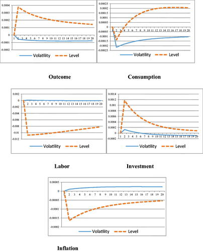
Figure 2 shows the macroeconomic effects of level shocks and volatility shocks under a prudent monetary policy. Level shocks and volatility shocks have the same conclusions as positive monetary policies: level shocks are a positive effect and have a larger impact; volatility shocks are a negative effect and have a smaller impact. On the order of magnitude, the economic effects of fluctuations under a stable monetary policy are greater than those of an active monetary policy. Compared with the proactive monetary policy, under the prudent monetary policy, the welfare loss caused by fluctuations is greater. Therefore, proactive monetary policy is more effective in the face of fluctuations.

Figure 2. Macroeconomic Effects of Level Shocks and Volatility Shocks (Prudent Monetary Policy). Source: The Authors.

Further, this article uses the lifetime effect of a representative family to measure the welfare level, and uses the welfare loss as a standard to evaluate the level effects and volatility effects. Define the welfare loss function: $$L=E_t\sum _{i=1}^n{\theta }^i({\pi }_{t+i}^2+\lambda y_{t+i}^2)$$ where $\theta$ is a discount factor between 0 and 1, $\lambda$ characterises the relative focus of central banks on output, and $n$ is the time range. In most cases, it is assumed that the maximum value of $n$ is $\infty .$ The maximum value set in this article is 20, which is consistent with the time range of the previous impulse response graph. Suppose the central bank has the same time preference as the family, $\theta =\beta ,$ three intervals $\mathrm{(}0,1\mathrm{)},1,(1,\infty ),$ Select $\lambda =0.5,\lambda =1.0,\lambda =2.0$ for analysis.

From the comparison of welfare losses in Table 3, we find that the welfare losses caused by shocks at levels of $\lambda =0.5,\lambda =1.0,\lambda =2.0$ are all greater than volatility shocks, about an order of magnitude. This is also consistent with the conclusions of Fernández-Villaverde, Guerrón-Quintana, Rubio-Ramirez, et al. (2011).

Table 3. Welfare loss comparison.

	Positive policy		Prudent policy
	Level shock	Volatility shock	Level shock	Volatility shock
λ = 0.5	5.11E-07	3.08E-08	6.04E-07	5.76E-08
λ = 1.0	9.36E-07	5.88E-08	1.06E-06	1.07E-07
λ = 2.0	1.79E-06	1.15E-07	1.96E-06	2.05E-07

Source: The Authors.

By comparing the impulse response of level shocks and volatility shocks of the technology, it can be found that the volatility shocks have completely different effect from the level shocks: the level shocks are a direct effect, the positive effect, the greater the impact; the volatility shocks are an indirect effect, the negative effect, the impact is small. From an order of magnitude, the impact of level technology on the real economy is greater than the impact of fluctuations. Fernández-Villaverde, Guerrón-Quintana, Rubio-Ramirez, et al. (2011) believes that this is mainly due to the direct impact of level shocks on the real economy, while uncertain shocks affect households and businesses’ expectations of the future and thus their production behaviours, and ultimately achieve physical economic influence, which is an indirect way of influence; this communication channel is relatively weak.

6. Conclusion

Actual business cycle theory and neo-Keynesian business cycle theory both assume that exogenous shocks are homogeneous shocks with constant volatility and ignore the heterogeneous shocks of time-varying volatility. Only the level effect of uncertainty shock is measured; the volatility effect of uncertainty shock cannot be measured. Based on micro-foundations, incorporating uncertainty shock into the research framework of D.S.G.E. model, and studying its impact on macroeconomic operations and policy responses are the key issues in the international academic community in recent years. However, most of the research is aimed at developed countries dominated by the U.S., without re-modeling specifically for the economic characteristics of developing countries such as China.

Based on the research ideas of Bloom (2009) and Fernández-Villaverde, Guerrón-Quintana, Rubio-Ramirez, et al. (2011), this article introduces the time-varying volatility model into a D.S.G.E. model, and uses the third-order perturbation method to decompose the level and volatility effects of uncertainty shock. The empirical study of the impact of uncertainty shocks on China’s macroeconomic fluctuations is based on Chinese data. The results show that volatility shocks have completely different effect from level shocks: the effect of level shocks is direct and positive, and their impact is larger; while the effect of volatility shocks is indirect and negative, and their impact is smaller; the volatility shocks will cause inflation while causing economic stagnation, which will produce a ‘stagflation’ effect. The research in this article shows that prudent monetary policy has the same research conclusions as active monetary policy, but the welfare loss caused by it is greater, so active monetary policy is more effective in the face of fluctuations.

China’s economy has changed from a stage of high-speed growth to a stage of high-quality development. High-quality development is key to China’s economic and social operation, which is the only way for high-quality development, whether to deal with external shocks or to prevent and control major risks. By measuring the level effect and volatility effect of uncertainty impact, this article can help us better understand the risks in high-quality economic development. When major emergencies such as S.A.R.S., the Wenchuan earthquake or C.O.V.I.D.-19 occur, the effect of the sudden impact on China’s macro economy is negative. In conclusion, through the comparison between positive monetary policy and stable monetary policy, the effect of positive monetary policy is better. The following aspects are worthy of in-depth study. Firstly, model settings such as fiscal policy, open economy, and financial friction can be considered. Secondly, based on the perspective of uncertainty shocks, study can be considered of the successful experience and failed lessons of the Chinese government in coping with the international financial crisis under the Hong Kong financial crisis, the U.S. financial crisis, and the European debt crisis. Thirdly, it is worthwhile studying the explanation of the ‘liquidity trap’ and ‘uncertainty trap’ for the current sluggish economic growth in China. Research on the macroeconomic effects of uncertain impacts at other levels is also meaningful, such as macro policy and investment. It is hoped that this article will play a role in attracting new ideas and promoting further research results.

Disclosure statement

No potential conflict of interest was reported by the authors.

Additional information

Funding

This work was supported by the Outstanding Youth Program of Zhejiang Natural Science Foundation under Grant LR20G030001; Zhejiang Social Science Foundation under Grant 19NDJC198YB; First Class Discipline of Zhejiang – A (Zhejiang Gongshang University – Statistics); Graduate Innovation Fund of Zhejiang Gongshang University; and Modern Business Center of Zhejiang Gongshang University.

References

- Alessandri, P., & Mumtaz, H. (2019). Financial regimes and uncertainty shocks. Journal of Monetary Economics, 101, 31–46. https://doi.org/https://doi.org/10.1016/j.jmoneco.2018.05.001
- Andreasen, M. M. (2012). On the effects of rare disasters and uncertainty shocks for risk premia in non-linear DSGE models. Review of Economic Dynamics, 15(3), 295–316. https://doi.org/https://doi.org/10.1016/j.red.2011.08.001
- Arellano, C., Bai, Y., & Kehoe, P. (2012). Financial markets and fluctuations in uncertainty. Research Department Staff Report. Federal Reserve Bank of Minneapolis.
- Bachmann, R., & Bayer, C. (2011). Uncertainty business cycles – Really? Social Science Electronic Publishing.
- Bachmann, R., & Moscarini, G. (2011). Business cycles and endogenous uncertainty. Meeting Papers 36. Society for Economic Dynamics.
- Basu, S., & Bundick, B. (2017). Uncertainty shocks in a model of effective demand. Econometrica, 85(3), 937–958. https://doi.org/https://doi.org/10.3982/ECTA13960
- Basu, S., & Bundick, B. (2012). Uncertainty shocks in a model of effective demand. NBER Working Papers 18420. National Bureau of Economic Research, Inc.
- Bloom, N. (2014). Fluctuations in uncertainty. Journal of Economic Perspectives, 28(2), 153–176. https://doi.org/https://doi.org/10.1257/jep.28.2.153
- Bloom, N., Floetotto, M., Jaimovich, N., Saporta Eksten, I., & Terry, S. (2012). Really uncertain business cycles. Social Science Electronic Publishing.
- Bloom, N. (2009). The impact of uncertainty shocks. Econometrica, 77(3), 623–685.
- Bonciani, D., & Van Roye, B. (2013). Uncertainty shocks, banking frictions, and economic activity. Kiel Working Paper No. 1843. Kiel Institute for the World Economy (IfW).
- Born, B., & Peifer, J. (2011). Policy risk and the business cycle. Bonn Econ Discussion Papers No. 06/2011. University of Bonn, Bonn Graduate School of Economics (BGSE).
- Brede, M. (2013). Disaster risk in a New Keynesian model. SFB 649 Discussion Paper Disaster risk in a New Keynesian model (No. 2013-020). Humboldt-Universität zu Berlin.
- Calvo, G. A. (1983). Staggered prices in a utility-maximizing framework. Journal of Monetary Economics, 12(3), 383–398. https://doi.org/https://doi.org/10.1016/0304-3932(83)90060-0
- Carrière-Swallow, Y., & Céspedes, L. F. (2013). The impact of uncertainty shocks in emerging economies. Journal of International Economics, 90(2), 316–325. https://doi.org/https://doi.org/10.1016/j.jinteco.2013.03.003
- Cesa-Bianchi, A., Corugedo, E. F. (2014). Uncertainty in a model with credit frictions. Social Science Electronic Publishing.
- Christiano, L., Motto, R., & Rostagno, M. (2014). Risk shocks. American Economic Review, 104(1), 27–65. https://doi.org/https://doi.org/10.1257/aer.104.1.27
- Cuaresma, J. C., Huber, F., & Onorante, L. (2020). Fragility and the effect of international uncertainty shocks. Journal of International Money and Finance, 1(1), 1–29. https://doi.org/https://doi.org/10.1016/j.jimonfin.2020.102151
- Davig, T., & Foerster, A. T. (2014). Uncertainty and fiscal cliffs. SSRN Electronic Journal, 10(3), 53–60.
- Fang, F. Q., & Wang, Q. (2012). Dynamic Stochastic general equilibrium modeling: Literature study and future prospects. Economic Theory and Business Management, 2012(11), 34–50.
- Fernández-Villaverde, J., Guerrón-Quintana, P. A., Kuester, K., & Rubio-Ramírez, J. (2011). Fiscal volatility shocks and economic activity. NBER Working Paper No. w17317. National Bureau of Economic Research.
- Fernández-Villaverde, J., Guerrón-Quintana, P., Rubio-Ramirez, J. F., & Uribe, M. (2011). Risk matters: the real effects of volatility shocks. Social Science Electronic Publishing.
- Gilchrist, S., Sim, J., & Zakrajsek, E. (2014). Uncertainty, financial frictions, and investment dynamics. SSRN Electronic Journal, 2014(11), 31–49.
- Gupta, R., Olasehinde-Williams, G., & Wohar, M. E. (2020). The impact of US uncertainty shocks on a panel of advanced and emerging market economies. The Journal of International Trade & Economic Development, 2020(1), 1–11.
- Jin, Z. X., Hong, H., & Li, H. J. (2013). The effectiveness of interest rate liberalization. Economic Research Journal, 2013(4), 70–83.
- Judd, K. L., & Guu, S. M. (1997). Asymptotic methods for aggregate growth models. Journal of Economic Dynamics and Control, 21(6), 1025–1042. https://doi.org/https://doi.org/10.1016/S0165-1889(97)00015-8
- Jurado, K., Ludvigson, S. C., & Ng, S. (2015). Measuring uncertainty. American Economic Review, 105(3), 1177–1177. https://doi.org/https://doi.org/10.1257/aer.20131193
- Keen, B. D., & Pakko, M. R. (2011). Monetary policy and natural disasters in a DSGE model. Southern Economic Journal, 77(4), 973–990. https://doi.org/https://doi.org/10.4284/0038-4038-77.4.973
- Kim, J., Kim, S. H., & Levin, A. (2003). Patience, persistence, and welfare costs of incomplete markets in open economies. Journal of International Economics, 61(2), 385–396. https://doi.org/https://doi.org/10.1016/S0022-1996(03)00009-6
- Leduc, S., & Liu, Z. (2016). Uncertainty shocks are aggregate demand shocks. Journal of Monetary Economics, 82, 20–35. https://doi.org/https://doi.org/10.1016/j.jmoneco.2016.07.002
- Li, C., Ma, W. T., & Wang, B. (2010). Inflation Expectation, the Selection of Monetary Policy Instruments and Economy Stability. China Economic Quarterly, 10(1), 51–82.
- Liu, B. (2008). Development of DSGE model in China and its application in monetary policy analysis. Journal of Financial Research, 2008(10), 5–25.
- Liu, B. (2010). Dynamic stochastic general equilibrium model and its application. China Finance Press.
- Liu, J. Q., & Pan, F. H. (2012). On the links between inflation, output and uncertainty: VAR-GARCH tests for the China’s Economy. Jilin University Journal Social Sciences Edition, 52(3), 89–93.
- Ma, W. T. (2010). Inflation uncertainty and its effects on macroeconomy. Journal of Zhongnan University of Economics and Law, 2010(2), 9–14.
- Ma, W. T., & Wei, F. C. (2011). Measurement of quarterly output gap based on new Keynes dynamic stochastic general equilibrium model. Management World, 2011(5), 39–65.
- Mei, D. Z., & Gong, L. T. (2011). The determinants of exchange rate regime in the emerging economies. Economic Research Journal, 2011(11), 73–88.
- Mumtaz, H., & Zanetti, F. (2013). The impact of the volatility of monetary policy shocks. Journal of Money, Credit and Banking, 45(4), 535–558. https://doi.org/https://doi.org/10.1111/jmcb.12015
- Rotemberg, J. J. (1982). Sticky prices in the United States. Journal of Political Economy, 90(6), 1187–1211. https://doi.org/https://doi.org/10.1086/261117
- Shen, Y., Li, S. K., & Ma, X. T. (2012). The evolution and latest development of VAR macro econometric model. Journal of Quantitative & Technical Economics, 2012(10), 151–161.
- Schmitt-Grohé, S., & Uribe, M. (2004). Solving dynamic general equilibrium models using a second-order approximation to the policy function. Journal of Economic Dynamics and Control, 28(4), 755–775. https://doi.org/https://doi.org/10.1016/S0165-1889(03)00043-5
- Swanson, E. T. (2012). Risk aversion and the labour margin in dynamic equilibrium models. American Economic Review, 102(4), 1663–1691. https://doi.org/https://doi.org/10.1257/aer.102.4.1663
- Tang, W. J., Liao, R. R., & Liu, J. (2009). A review of studies on the economic impact of public emergencies. Economic Developments, 2009(4), 114–118.
- Tang, W. J., Xie, H. L., & Xu, X. W. (2012). Review of research on sudden impacts of impacting economy. Economic Developments, 2012(3), 149–154.
- Yang, L., & Li, L. (2011). Money shock and Chinese economic fluctuations-quantitative analysis based on a DSGE model. Modern Economic Science, 2011(5), 1–9.
- Yuan, S. G., Chen, P., & Liu, L. F. (2011). Exchange rate system, financial accelerator and economical undulation. Economic Research Journal, 2011(1), 59–72.
- Zhang, W. P. (2012). Monetary policy theory: A dynamic general equilibrium approach. Peking University Press.
- Zhang, S., Liu, Y., & Huang, D. H. (2019). Contribution of factor structure change to China’s economic growth: evidence from the time-varying elastic production function model. Economic Research-Ekonomska Istraživanja, 10(1), 1–24.
- Zheng, Y. Y. (2010). Theory of impulse response function with application in macroeconomics. Nankai University.