Dynamic behaviour of optimal portfolio with stochastic volatility

Abstract

In the existing literature, little is known about the dynamic behaviour of the optimal portfolio in terms of market inputs and arbitrary stochastic factor dynamics in an incomplete market with a stochastic volatility. In this paper, to study optimal portfolio behaviour, we compute and analyze the mean and the variance of the optimal portfolio and of their adjustment speed in terms of market inputs in an incomplete market. The incompleteness arises from the additional source of uncertainty of the volatility in Heston’s stochastic volatility model. Conducting sensitivity analysis for the mean and the variance of the optimal portfolio process as well as its adjustment speed to the market parameters, we find several interesting behavioural patterns of investors towards asset price and its volatility shocks. Our results are robust and convergent by the agreement from two simulation methods for different time step increments and the number of Monte Carlo simulation paths.

Keywords:

• Portfolio selection
• portfolio distribution
• dynamic behaviour
• Heston Stochastic volatility model
• incomplete market

JEL CODES:

• G11
• G12
• C63

View Expression of Concern:

Expression of Concern

1. Introduction

The volatility and anomalies of the stock market have been the focus of study since the global financial crisis, especially in emerging Asian financial markets (Gulzar et al., 2019; Zaremba & Nikorowski, 2019). The questions of the sensitivity of the optimal portfolio choice and investors’ behaviour in terms of the market parameters, stochastic factor and risk preferences are central in financial economics and have been studied primarily in simple economical models (see for example, Kimball (1990) and Landsberger and Meilijson (1990) and references therein). Kimball (1990) used ’prudence’ as a measure of the sensitivity of optimal choices to risk and focussed on precautionary saving. Landsberger and Meilijson (1990) studied conditions on distributions and concave utility functions under which investors would demand more of a (risky) asset. For other types of risky asset portfolio choice, Kołodziejczyk et al. (2019) studied Polish real estate portfolio allocation and Nicolae and Maria-Daciana (2019) studied currency risk portfolios in Romania.

For diffusion models with and without a stochastic factor, some qualitative results about optimal portfolios can be found in Borrell (2007), Detemple et al. (2003), Kim and Omberg (1996), Liu (2007) and Wachter (2002). Borrell (2007) studied the monotonicity properties of optimal portfolios in the classical utility maximisation problem of terminal wealth and confirmed that the optimal portfolio in terms of the total wealth invested in a given risk asset at any date was decreasing in wealth. Detemple et al. (2003) studied the economic properties of optimal portfolios in complete markets. Kim and Omberg (1996) and Wachter (2002) discussed dynamic portfolio behaviour in terms of the stochastic risk premium (in fact, market price of risk) following the simplest mean-reverting diffusion process, and Wachter (2002) obtained a closed form solution for optimal portfolios under the assumption of a complete market. Bergen et al. (2018) provided optimal multivariate intertemporal portfolios for an ambiguity averse investor, who has access to stocks and derivative markets, in closed form. In Escobar et al. (2017), a stochastic covariance model is studied and implemented for incomplete and complete markets. Fouque et al. (2017) presented a formal derivation of asymptotic approximations for portfolio optimisation with stochastic volatility asymptotic. For recent empirical research on multi-asset portfolio asset allocation, we refer the work of Isiksal et al. (2019).

However, little is known about the dynamic behaviour of the optimal portfolio in terms of market inputs and arbitrary stochastic factor dynamics in an incomplete market with a stochastic volatility. As pointed out by Zariphopoulou (2009), computing and analyzing the distribution of the portfolio process as well as its moments were open questions. In this paper we will address these questions in the framework of the Heston’s stochastic volatility model.

The Black-Scholes model, a famous mathematical options pricing model in the field of financial economics, was developed by Black and Scholes (1973). It provides a theoretical estimate of the price of European option with the assumption that stock returns are normally distributed with known mean and variance. Under this assumption, price volatility is constant. However, this assumption needs to be fully considered since volatility plays a crucial role in determining the price of an option and risk management. To better describe the real-world economic phenomena, Hull and White generalise the model with the development of the stochastic volatility model in 1987. But their model has its own disadvantages in that it does not have a closed-form solution and requires solving two-dimension partial differential equations. To solve this problem, Stein and Stein (1991) assumed that volatility was uncorrelated with the spot asset. However, their method failed to capture the important skewness effects arising from such correlations. Subsequently, Heston (1993) developed a new model, now known as Heston’s stochastic volatility model, allowing an arbitrary correlation between the risky asset and its volatility. In that model, the Cox-Ingersoll-Ross (CIR) process was employed to formulate the volatility and its correlation with the risky asset price (or return). Under such a condition, since there is one risky asset being traded with two sources of uncertainty (namely, the uncertainty of the risky asset’s price and the uncertainty of the volatility), the market is incomplete and no unique equivalent martingale measure exists. Under the assumption of bounded market price of risk, Kraft (2005) obtained a closed form solution for the optimal portfolio. The closed-form solution allows us to further study the distribution and moments of the optimal portfolio process as well as its adjustment speed in response to the market conditions.

The remainder of the paper is structured as follows. In section 2, we describe the general framework of a continuous-time financial market that consists of one risk-free bond and one risky asset, as well as the maximisation problem in the incomplete market. In section 3, we study the impact of market parameters on the percentage change of the optimal portfolio weight invested in the risky asset. In section 4, we conduct numerical simulations for time dependent paths, the mean and variance of optimal portfolio process followed by the study of the sensitivity of these paths to the market parameters. Robustness and convergence tests are also performed by comparing different simulation methods, namely, the time step size and the number of Monte Carlo paths. Finally, we conclude the paper in section 5.

2. The closed form solution of optimal portfolio

We consider a continuous-time financial market consisting of a risk-free bond and a risky asset (or stock).

The price, denoted by B, of the risk-free bond, which offers a time-dependent nominal interest rate of r(t), satisfies (1) $$\frac{dB(t)}{B(t)}=r(t)dt.$$(1)

The price, denoted by S, of the risky asset follows Heston’s stochastic volatility model given by (2) $$\begin{array}{c}\frac{dS(t)}{S(t)}=\mu (t)dt+\sqrt{v(t)}\left(\rho d{W}_1(t)+\sqrt{1-{\rho }^2}d{W}_2(t)\right)\hfill \\ dv(t)=\kappa (\theta -v(t))dt+\sigma \sqrt{v(t)}d{W}_1(t)\hfill \end{array}$$(2) where $\mu (t)$ is the expected nominal return on the stock, and ρ ($\rho \in [-1,1]$) is an arbitrary correlation between the stock return and the stock volatility. The parameters $\kappa ,\theta ,\sigma >0$ and θ correspond to the long-run variance while κ controls the speed, by which the variance v(t) returns to its long-run variance θ. The two independent Brownian motions, W₁ and W₂, are defined on a probability space ($\Omega ,\mathcal{F},P$) and $\mathcal{F}{(t)}_{t\ge 0}$ is the P-augmentation of the Brownian filtration.

Let us assume that, at time $t\in [0,T]$ for a fixed T, a representative investor with an initial wealth $x\ge 0$ invests a proportion $\pi (t)$¹ of his wealth into the stock and the remaining proportion $1-\pi (t)$ into the risk-free bond. The corresponding wealth process X(t) must then satisfy (3) $$\begin{array}{c}\frac{dX(t)}{X(t)}=\left[r(t)+\pi (t)(\mu (t)-r(t))\right]dt+\pi (t)\sqrt{v(t)}\left[\rho d{W}_1+\sqrt{1-{\rho }^2}d{W}_2(t)\right],\hfill \\ X_0=x.\hfill \end{array}$$(3)

The portfolio weight $\pi (t)$ satisfies the standard assumption of being $X(t)\ge 0$ self-financing² and is deemed admissible if the corresponding wealth process P-a.s. for all $t\in [0,T].$ We denote the set of admissible portfolio weights by $\mathcal{A}.$

Now consider the following maximisation problem maximising the expected utility of terminal wealth (4) $$\underset{\pi (t)\in \mathcal{A}}{\max }\mathbb{E}[u(X(T))]$$(4) subject to (3). The utility function $u:(0,+\infty )\to \mathbb{R}$ is increasing ($u\prime >0$), concave ($u″<0)$³ and satisfies the following Inada conditions $$\underset{x\to 0}{\lim }u\prime (x)=+\infty$$ and $$\underset{x\to \infty }{\lim }u\prime (x)=0.$$

Consider the maximisation problem of (4) subject to (3) in the incomplete market of (1) and (2) with the CRRA utility function defined by⁴ (5) $$u(x)=\frac{x^{1-\gamma }}{1-\gamma },\hspace{1em}\gamma >0\mathrm{}\text{and}\mathrm{}\gamma \ne 1^4.$$(5)

Under the assumption of bounded market price of risk, Kraft (2005) shows that the optimal proportion ${\pi }^{*}(t)$ in stock is given by (6) $${\pi }^{*}(t)=\frac{1}{\gamma }\frac{\mu (t)-r(t)}{v(t)},$$(6) with the variance v(t) satisfying ⁵ (7) $$dv(t)=\kappa (\theta -v(t))dt+\sigma \sqrt{v(t)}d{W}_1(t).$$(7)

Note the above result is the same as Equation (32) in Proposition 6.1 in Kraft (2005).

3. Dynamics and behaviour of the adjustment speed of the optimal portfolio process

Applying the $It\widehat{o}$ lemma to the optimal portfolio ${\pi }^{*}(t)$ in (6) and using (7), we obtain (8) $$\frac{d{\pi }^{*}(t)}{{\pi }^{*}(t)}=\left(\frac{e\prime (t)}{e(t)}+\frac{{\sigma }^2-\kappa (\theta -v(t))}{v(t)}\right)dt-\frac{\sigma }{\sqrt{v(t)}}d{W}_1(t),$$(8) where, $e(t)=\mu (t)-r(t)$ is the expected excess return on the stock and positive (negative) if the expected stock return is greater (less) than the risk-free rate, i.e, $\mu (t)>(<)r(t).$ The symbols ($\prime$) denotes the first derivative.

We define $\frac{d{\pi }^{*}(t)}{{\pi }^{*}(t)}/dt$ as the portfolio adjustment speed which measures the percentage change of the optimal portfolio weight invested in the stock.

Before studying the distribution and behaviour of the optimal portfolio process in the following section, we first analyze below the mean and variance of the portfolio adjustment speed, as well as its behaviour in terms of market inputs.

Letting the variance of the stock return converge to its long-run variance, i.e., $v\to \theta ,$ we have (9) $$\frac{d{\pi }^{*}(t)}{{\pi }^{*}(t)}=\left(\frac{e\prime (t)}{e(t)}+\frac{{\sigma }^2}{\theta }\right)dt-\frac{\sigma }{\sqrt{\theta }}d{W}_1(t).$$(9)

Dividing (9) by dt and then taking expectation and variance, respectively, give (10) $$\begin{array}{c}E\left[\frac{d{\pi }^{*}(t)}{{\pi }^{*}(t)}/dt\right]=\frac{e\prime (t)}{e(t)}+\frac{{\sigma }^2}{\theta },\hfill \\ \mathit{Var}\left[\frac{d{\pi }^{*}(t)}{{\pi }^{*}(t)}/dt\right]=\frac{{\sigma }^2}{\theta }/dt.\hfill \end{array}$$(10)

Therefore, both the mean and variance of the portfolio adjustment speed increase with the volatility of volatility σ, and decrease with the long-run variance θ.

For the general case with $t_0\le t\le t_0+dt,$ dividing (8) by dt and then taking expectation and variance, respectively, give⁶ (11) $$\begin{array}{c}E\left[\frac{d{\pi }^{*}(t)}{{\pi }^{*}(t)}/dt\right]=\frac{e\prime (t)}{e(t)}+\frac{{\sigma }^2-\kappa (\theta -v(t_0))}{v(t_0)},\hfill \\ \mathit{Var}\left[\frac{d{\pi }^{*}(t)}{{\pi }^{*}(t)}/dt\right]=\frac{{\sigma }^2}{v(t_0)}/dt.\hfill \end{array}$$(11)

From the relationships in (11), we can discuss the impact of the model parameters on the portfolio weight adjustment speed as follows:

• The expected portfolio adjustment speed $E[\frac{d{\pi }^{*}(t)}{{\pi }^{*}(t)}/dt]$ is an increasing function of $\frac{e\prime (t)}{e(t)}$ which measures the rate of change of expected excess return. Obviously, when the expected excess return increases at a faster rate, investors will increase the weight of risky asset in their portfolio at a faster rate.

• The expected portfolio adjustment speed $E[\frac{d{\pi }^{*}(t)}{{\pi }^{*}(t)}/dt]$ is an increasing function of κ when $v(t_0)>\theta .$ For increasing κ, v reverts downward to θ at a faster rate, then the stock becomes less risky at a faster rate. Thus, the investor increases the weight invested in the less risky stock at a faster rate. This can be explained intuitively as follows: When an economic shock occurs, the volatility of the stock market increases above the long-term equilibrium level, i.e., $v(t_0)>\theta .$ The mean reversion speed κ depends on the size of the economic shock. Thus, we can regard κ as a measure of the economic recovery speed. Therefore, the smaller the shock, the quicker the economy will recover back to the normal state and the volatility of the stock market will revert back to the long-term level. Under such conditions, the investor quickly rebalances their portfolio weight as they anticipate the market returning to a normal state as the economic shock is small and transient. Conversely, when the strength of the shock is large, such as the 2008 financial crisis, the investor anticipates a slow economic recovery, generating a small mean reversion speed κ and so the investor rebalances their portfolio in a more gradual way.

• The expected portfolio adjustment speed $E[\frac{d{\pi }^{*}}{{\pi }^{*}}/dt]$ is a decreasing function of κ when $v(t_0)<\theta .$ For increasing κ, v reverts upward to θ at a faster rate, then the stock becomes riskier at a faster rate. The investor decreases the weight invested in the riskier stock at a faster rate. During a period of slow economy growth, the stock market has lower than normal long-term volatility. When the economic growth picks up speed towards the normal growth rate, the stock market tends to become more volatile and the investor sells off some of the stock due to risk aversion. The sell-off speed will depend on how quickly the market volatility increases to the normal risk level.

• Both the expected portfolio adjustment speed $E[\frac{d{\pi }^{*}(t)}{{\pi }^{*}(t)}/dt]$ and the variance of the portfolio adjustment speed $\mathit{Var}[\frac{d{\pi }^{*}}{{\pi }^{*}}/dt]$ increase with the volatility of volatility σ (or variance of volatility ${\sigma }^2$). In other words, when the price risk becomes more uncertain, investors tend to increase their weight in the risky asset at a faster rate and thus the adjustment rate becomes more uncertain. It is interesting to see that investors like the volatility of the volatility. Due to their risk aversion, investors reduce their portfolio risk by selling a certain amount of the risky asset when its risk level (price variance) increases. But the more this risk-level volatility increases, the less amount of risky asset investors will sell because they believe that such risk level increase has high uncertainty and the risk level could soon decrease.

• The expected portfolio adjustment speed $E[\frac{d{\pi }^{*}(t)}{{\pi }^{*}(t)}/dt]$ is a decreasing function of θ. As the long-run variance θ of the stock increases, the investor tends to invest less into it to avoid risk.

4. The distribution and dynamic behaviour of the optimal portfolio process

In this section, we compute and analyze the time-dependent paths of the mean and the variance of the optional portfolio process ${\pi }^{*}(t)$ using numerical simulations. We further examine the dynamic behaviour of the optimal portfolio process by investigating the sensitivity of the mean and the variance to the market inputs.

From (8), we can obtain (12) $$d\hspace{0.17em}\text{ln}\hspace{0.17em}({\pi }^{*}(t))=\left(\frac{e\prime (t)}{e(t)}+\frac{\frac{1}{2}{\sigma }^2-\kappa (\theta -v(t))}{v(t)}\right)dt-\frac{\sigma }{\sqrt{v(t)}}d{W}_1(t).$$(12)

Integrating (12) gives (13) $${\pi }^{*}(t)={\pi }^{*}(0)\frac{e(t)}{e(0)}\text{exp}\hspace{0.17em}\left\{{\int }_0^t\frac{\frac{1}{2}{\sigma }^2-\kappa (\theta -v(s))}{v(s)}ds-{\int }_0^t\frac{\sigma }{\sqrt{v(s)}}d{W}_1(s)\right\}.$$(13)

When the variance v(t) approaches the long-run variance θ, we can get (14) $${\pi }^{*}(t)={\pi }^{*}(0)\frac{e(t)}{e(0)}\text{exp}\hspace{0.17em}\left\{\frac{{\sigma }^2}{2\theta }t-\frac{\sigma }{\sqrt{\theta }}{W}_1(t)\right\}.$$(14)

Taking expectation and variance, respectively, we obtain (15) $$\begin{array}{c}E[{\pi }^{*}(t)]={\pi }^{*}(0)\frac{e(t)}{e(0)}\text{exp}\hspace{0.17em}\left\{\frac{{\sigma }^2}{\theta }t\right\},\hfill \\ \mathit{Var}\left[{\pi }^{*}(t)\right]={\left({\pi }^{*}(0)\frac{e(t)}{e(0)}\right)}^2\left(\hspace{0.17em}\text{Exp}\hspace{0.17em}\left\{\frac{3{\sigma }^{2}t}{\theta }\right\}-\hspace{0.17em}\text{Exp}\hspace{0.17em}\left\{\frac{2{\sigma }^{2}t}{\theta }\right\}\right),\hfill \end{array}$$(15) for $v\to \theta .$ When volatility v(t) is not near θ, we adopt the Monte Carlo simulation method.

4.1. Monte Carlo simulation for the optimal portfolio process distribution

To apply the Monte Carlo simulation method to simulate the mean and variance of the optimal portfolio process ${\pi }^{*}(t),$ we discretize the volatility equation in (7) as (16) $$v^{(j)}(t_i)-v^{(j)}(t_{i-1})=\kappa [\theta -v^{(j)}(t_{i-1})]\Delta t+\sigma \sqrt{v^{(j)}(t_{i-1})}\Delta t·Z_i^{(j)}$$(16) where $i=1,2,···,N,\hspace{1em}j=1,2,···,M.$ N is the number of time steps, M is the number of Monte Carlo paths, $\Delta t$ is the time step size, and $Z_i^{(j)}$ is a standard normally-distributed random variable.

To simplify notations, we define the following variables: $$\begin{array}{c}f(v)=\frac{\frac{1}{2}{\sigma }^2-\kappa (\theta -v(t))}{v(t)},\hfill \\ g(v)=\frac{\sigma }{\sqrt{v(t)}},\hfill \\ Y(t_n)={\int }_0^{t_n}f(v)dt-{\int }_0^{t_n}g(v)d{W}_1(t),\hspace{1em}n=1,2,···,N.\hfill \end{array}$$

Then from (13) we can get (17) $${\pi }^{*}(t_n)={\pi }^{*}(0)\frac{e(t)}{e(0)}\text{exp}\hspace{0.17em}\{Y(t_n)\}.$$(17)

The numerical approximation of $Y(t_n)$ is given by (18) $$Y^{(j)}(t_n)=\sum _{i=1}^{n}f(v^{(j)}(t_{i-1}))\Delta t-\sum _{i=1}^{n}g(v^{(j)}(t_{i-1}))\sqrt{\Delta t}·Z_i^{(j)}.$$(18)

Taking expectation and variance of (17), we obtain (19) $$\begin{array}{c}E[{\pi }^{*}(t_n)]\approx {\pi }^{*}(0)\frac{e(t)}{e(0)}\frac{1}{M}\sum _{j=1}^{M}Exp\{Y^{(j)}(t_n)\},\hfill \\ \mathit{Var}[{\pi }^{*}(t_n)]=E\left[{({\pi }^{*}(t_n))}^2\right]-{\left\{E\right[{\pi }^{*}(t_n)\left]\right\}}^2,\hfill \\ E\left[{({\pi }^{*}(t_n))}^2\right]\approx {\left({\pi }^{*}(0)\frac{e(t)}{e(0)}\right)}^2\frac{1}{M}\sum _{j=1}^{M}Exp\{2Y^{(j)}(t_n)\}.\hfill \end{array}$$(19)

4.2. The dynamic behaviour of the optimal portfolio process in terms of market inputs

Our sensitivity analysis is conducted for various mean reversion speed κ, long-run expected variance θ, and the volatility of volatility σ. Our simulations are carried out on a daily basis with a time step size $\Delta t=\frac{1}{365},$ with the number of Monte Carlo paths M = 500, and an initial weight ${\pi }^{*}(0)=0.6.$ Since our main goal is to study portfolio behaviour for the different input parameters of the volatility model (7), we hold the expected excess return e(t) fixed which is assumed in Heston model.⁷

Figure 1 shows the time-depend paths for the mean and the variance of the optimal weights ${\pi }^{*}(t)$ for three different reversion speed $\kappa =0.1,0.2,0.5$ with θ and σ fixed. We set $\theta =0.04,\sigma =0.02$ and the initial variance $v(0)=0.02,$ which is smaller than the long-run variance $\theta =0.04.$ We observe that $E[{\pi }^{*}(t)]$ decreases with time to the equilibrium weight of 0.3 at a faster rate when κ increases. This is reasonable because κ controls the speed by which v(t) returns to its long-run variance θ, which in turn drives ${\pi }^{*}(t)$ to a long-run equilibrium as well. But the most interesting aspect is the evolution of $\mathit{Var}({\pi }^{*}(t)).$ We see that the variance rises very rapidly to relatively stable values for all three κ levels, and that variance falls as κ increases. 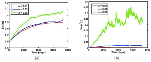Therefore the mean reversion speed κ not only drives the weight ${\pi }^{*}(t)$ to equilibrium at a faster rate but also impacts the stability of ${\pi }^{*}(t)$ with increasing stability as κ becomes larger. Figure 2 shows the case for $v(0)=0.06$ which is larger than $\theta =0.04$ while all other parameters are the same as in Figure 1. Here $E[{\pi }^{*}(t)]$ increases with time to equilibrium, and the effect of κ on $E[{\pi }^{*}(t)]$ for the case $v(0)=0.06$ is similar to the previous case of $v(0)=0.02.$ But the effect of κ on $\mathit{Var}({\pi }^{*}(t))$ is different as shown by comparing Figures 1(b) and 2(b) though $\mathit{Var}({\pi }^{*}(t))$ falls as κ increases in both cases.

Figure 1. Time-dependent paths of (a) mean, and (b) variance of the optimal weight ${\pi }^{*}(t)$ for the risky asset under three different mean reversion speed κ, with model parameters: ${\pi }^{*}(0)=0.6,v(0)=0.02<\theta =0.04,\sigma =0.02.$ Source: The authors.

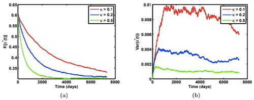
Figure 2. Time-dependent paths of (a) mean, and (b) variance of the optimal weight ${\pi }^{*}(t)$ for the risky asset under three different mean reversion speed κ, with model parameters: ${\pi }^{*}(0)=0.6,v(0)=0.06>\theta =0.04,\sigma =0.02.$ Source: The authors.

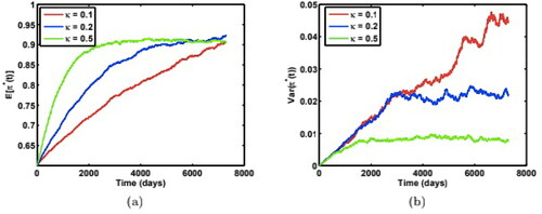
In the case $v(0)=0.06,\mathit{Var}({\pi }^{*}(t))$ increases at higher rate with the peak value of 0.05 than the case $v(0)=0.02$ where the peak value is around 0.01. This shows different investor behavioural patterns for two cases: (a) the asset becomes riskier as $v(0)=0.02$ increases to the larger long-run expected variance $\theta =0.04;$ (b) the asset becomes less risky as $v(0)=0.06$ decreases to the smaller long-run expected variance $\theta =0.04.$ As the asset gets less risky(case b), the investor increases the proportion invested in it in a more chaotic way than the case the investor sells their risky asset when the asset becomes riskier(case a). This shows that the investor has very different attitude towards buying assets when the market becomes less risky. On the other hand, when the market becomes more volatile, the investor will make similar strategy to sell assets from fear of market risk increasing.

Now we study the effect of the long-run variance θ on $E[{\pi }^{*}(t)]$ and $\mathit{Var}({\pi }^{*}(t)).$ Figure 3 shows the paths of the mean and variances of the optimal weight for three different $\theta (=0.01,0.04,0.09)$ with $v(0)=0.02,{\pi }^{*}(0)=0.6,\kappa =0.2,\sigma =0.02.$ Figure 4 shows the result for the case $v(0)=0.06$ in which all other parameters are the same as the case $v(0)=0.02.$ Here both cases of $v(0)=0.02,0.06$ display similar results. $E[{\pi }^{*}(t)]$ increases with decreasing long-run variance θ while $\mathit{Var}({\pi }^{*}(t))$ for small $\theta (=0.01)$ is much larger than at larger $\theta (=0.04,0.09).$ This shows that larger long-run variance has a stabilising effect on the weight path. This can be explained intuitively as follows. As an asset becomes riskier (larger θ), the investor will sell the risky asset in a homogeneous way (small variance) compared to the case when asset becomes less risky (smaller θ), in which the investor becomes greedy by over investing in the risky asset in a chaotic heterogenous way (large variance).

Figure 3. Time-dependent paths of (a) mean, and (b) variance of the optimal weight ${\pi }^{*}(t)$ for the risky asset under three different long-run variance θ, with model parameters: ${\pi }^{*}(0)=0.6,v(0)=0.02,\kappa =0.2,\sigma =0.02.$ Source: The authors.

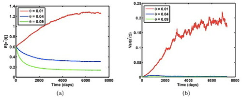
Figure 4. Time-dependent paths of (a) mean, and (b) variance of the optimal weight ${\pi }^{*}(t)$ for the risky asset under three different long-run variance θ, with model parameters: ${\pi }^{*}(0)=0.6,v(0)=0.06,\kappa =0.2,\sigma =0.02.$ Source: The authors.

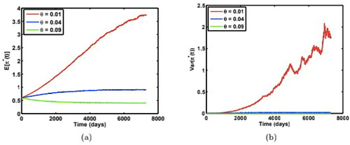
Finally, we study the impact of the volatility of volatility σ on the optimal weight paths. Figure 5 shows the case $v(0)=0.02$ and Figure 6 shows the case $v(0)=0.06.$ The simulations are carried out for three different $\sigma (=0.01,0.02,0.05)$ holding other parameters constant as: $({\pi }^{*}(0)=0.6,\kappa =0.2,\theta =0.04).$ The two cases $v(0)=0.02$ and $v(0)=0.06$ show similar qualitative characteristics for weight paths. $E[{\pi }^{*}(t)]$ decreases to equilibrium for $v(0)=0.02,$ but it increases to equilibrium for $v(0)=0.06.$ Here we find both $E[{\pi }^{*}(t)]$ and $\mathit{Var}({\pi }^{*}(t))$ increase with the volatility of volatility σ, and $\mathit{Var}({\pi }^{*}(t))$ becomes less stable with large σ. This result can be proved using (11) where both $E[\frac{d{\pi }^{*}}{{\pi }^{*}}/dt]$ and $\mathit{Var}\left(\frac{d{\pi }^{*}}{{\pi }^{*}}/dt\right)$ are monotone increasing functions of σ. Therefore, the investor tends to be optimistic when the volatility of risk is high by overinvesting in risky assets.

Figure 5. Time-dependent paths of (a) mean, and (b) variance of the optimal weight ${\pi }^{*}(t)$ for the risky asset under three different volatility of volatility σ, with model parameters: ${\pi }^{*}(0)=0.6,v(0)=0.02<\theta =0.04,\kappa =0.2.$ Source: The authors.

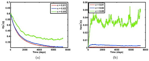
Figure 6. Time-dependent paths of (a) mean, and (b) variance of the optimal weight ${\pi }^{*}(t)$ for the risky asset under three different volatility of volatility σ, with model parameters: ${\pi }^{*}(0)=0.6,v(0)=0.06>\theta =0.04,\kappa =0.2.$ Source: The authors.

Further observations can be made about the difference of variance paths for two cases: (i) $v(0)<\theta ,$ and (ii) $v(0)>\theta$ as shown in Figures 1(b) and 2(b), Figures 3(b) and 4(b), and Figures 5(b) and 6(b). We find larger variances in case (ii) than case (i), which shows that the investor adjusts their weight in a more chaotic way when initial return risk is higher than the long run expected risk (case (ii)) than case (i). On the other hand, the variance paths in case (i) reach their maximal equilibrium at a much faster rate than in case (ii). This can be explained as follows. In case (i) $v(0)<\theta ,$ the investor will sell asset when the risk reverts upward to higher level θ while the investor will buy asset when risk reverts downward to lower level θ. The investor seems to react to risk increasing quicker than risk decreasing and sells asset in a more uniform way than they buy asset. This is in consistence with the behaviour of the stock market in the real world. The fall of the market is often faster than the rise.

4.3. Robustness and convergence tests

Here we introduce another way to compute $E[{\pi }^{*}(t)]$ and $\mathit{Var}[{\pi }^{*}(t)]$ to test robustness of our results obtained above. We refer the method described in Section 4.1 to as method 1, and the method described below as method 2.

From (6), we can obtain (20) $${\pi }^{*}(t)={\pi }^{*}(0)\frac{e(t)}{e(0)}v(0)\frac{1}{v(t)}.$$(20)

Taking expectation and variance, we get (21) $$\begin{array}{c}E[{\pi }^{*}(t_n)]={\pi }^{*}(0)\frac{e(t)}{e(0)}v(0)E\left[\frac{1}{v(t_n)}\right]\hfill \\ \approx {\pi }^{*}(0)\frac{e(t)}{e(0)}v(0)\frac{1}{M}\sum _{j=1}^M\frac{1}{v^{(j)}(t_n)}\hfill \end{array}$$(21) and (22) $$\begin{array}{c}\mathit{Var}[{\pi }^{*}(t_n)]=E\left[{({\pi }^{*}(t_n))}^2\right]-{\left\{E\right[{\pi }^{*}(t_n)\left]\right\}}^2,\hfill \\ E\left[{({\pi }^{*}(t_n))}^2\right]={({\pi }^{*}(0))}^2{\left(\frac{e(t)}{e(0)}\right)}^2{v}^2(0)E\left[\frac{1}{v^2(t_n)}\right]\hfill \\ \approx {({\pi }^{*}(0))}^2{\left(\frac{e(t)}{e(0)}\right)}^2{v}^2(0)\frac{1}{M}\sum _{j=1}^M\frac{1}{{(v^{(j)}(t_n))}^2}\hfill \end{array}$$(22) where $v^{(j)}(t_n)$ is obtained by (16) and M is the number of Monte Carlo paths.

For the illustration purpose, we only show the cases when the initial variance v(0) is below its long-run variance θ. Figures 7, 8, 9 show the comparison of the two methods for both mean and variance of the optimal weight paths ${\pi }^{*}(t)$ for the parameters: ${\pi }^{*}(0)=0.6,v(0)=0.02,\theta =0.04,\sigma =0.02$ and $\kappa =0.1,0.2,0.5$ respectively. We find the two methods yield almost the same results. Figure 10 shows the agreement of results for two different time steps $\Delta t=\frac{1}{12}$ (monthly) and $\Delta t=\frac{1}{365}$ (daily) with the same set of model parameters as in Figure 8. Figure 11 shows the agreement of results for two different numbers of Monte Carlo paths: $(M=500$ and $M=1000)$ for method 1 and Figure 12 shows the agreement of results for method 2.

Figure 7. Comparison of (a) mean weight paths, and (b) variance of weight paths from two numerical simulation methods to test for robustness, with model parameters: ${\pi }^{*}(0)=0.6,v(0)=0.02<\theta =0.04,\kappa =0.1,\sigma =0.02.$ Source: The authors.

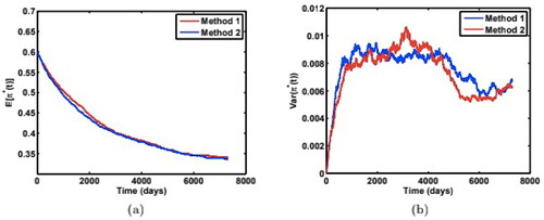
Figure 8. Comparison of (a) mean weight paths, and (b) variance of weight paths from two numerical simulation methods to test for robustness, with model parameters: ${\pi }^{*}(0)=0.6,v(0)=0.02<\theta =0.04,\kappa =0.2,\sigma =0.02.$ Source: The authors.

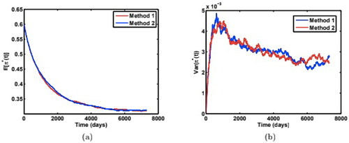
Figure 9. Comparison of (a) mean weight paths, and (b) variance of weight paths from two numerical simulation methods to test for robustness, with model parameters: ${\pi }^{*}(0)=0.6,v(0)=0.02<\theta =0.04,\kappa =0.5,\sigma =0.02.$ Source: The authors.

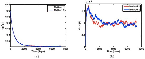
Figure 10. Comparison of (a) mean paths of weights, and (b) variance of weight paths from simulations using two different time steps (daily v.s. monthly) with model parameters: ${\pi }^{*}(0)=0.6,v(0)=0.02<\theta =0.04,\kappa =0.2,\sigma =0.02.$ Source: The authors.

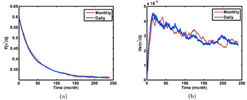
Figure 11. Comparison of (a) mean paths of weights, and (b) variance of weight paths from numerical simulations (method 1) for two different numbers of Monte Carlo simulation paths (M = 500 v.s. 1000) with model parameters: ${\pi }^{*}(0)=0.6,v(0)=0.02<\theta =0.04,\kappa =0.2,\sigma =0.02.$ Source: The authors.

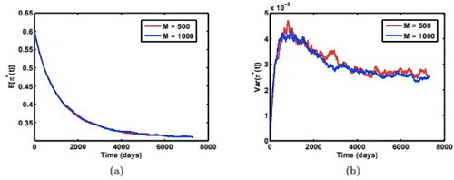
Figure 12. Comparison of (a) mean paths of weights, and (b) variance of weight paths from numerical simulations (method 2) for two different numbers of Monte Carlo simulation paths (M = 500 v.s. 1000) with model parameters: ${\pi }^{*}(0)=0.6,v(0)=0.02<\theta =0.04,\kappa =0.2,\sigma =0.02.$ Source: The authors.

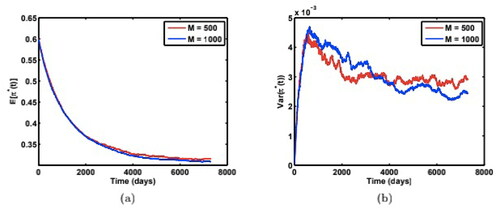
Therefore we can conclude that our results are both robust and convergent in terms of both the time steps and the number of Monte Carlo simulation paths.

5. Conclusion

We discuss the constraint maximisation problem of maximizing expected utility of terminal wealth in an incomplete market, where the incompleteness arises from the additional source of uncertainty of the volatility in Heston’s model. We first derive analytical formulas for the mean and the variance of the portfolio process and its adjustment speed, as well as sensitivities to the market parameters. We further conduct numerical simulations for the time-dependent paths for the mean and the variance of the optimal portfolio process. We also conduct a series of sensitivity analyses for the mean reversion speed, long-run expected variance and the volatility of volatility and show that these market parameters can have a significant impact on the investor’s behavioural patterns towards asset price and volatility shocks. Our results are robust and convergent by obtaining the agreement from two simulation methods for different time step increments and the numbers of Monte Carlo simulation paths.

Disclosure statement

No potential conflict of interest was reported by the author(s).

Additional information

Funding

The work is sponsored by K. C. Wong Magna Fund in Ningbo University, Ningbo-CASS collaborative grant NTZKT201701, Research Academy of Belt & Road of Ningbo University and Foundation of Zhejiang Educational Committee under grant Y201737633.

Notes

1 Here short-selling is allowed. That is, we do not impose that $\pi (t)\in [0,1].$

2 For the formal definition of a self-financing portfolio process please see, for example, Korn and Korn (2001) page 63.

3 An increasing utility implies that the investor prefers more to less, while a concave utility is associated with a risk-averse investor. The symbols ($\prime$) and ($″$) denote first and second derivative, respectively.

4 It is known that, when γ converges to 1 (or $\gamma \to 1$), the power utility function (5) simplifies to the log utility ln(x).

5 When the stock variance v(t) is constant, (6) becomes the well-know Merton’s portfolio rule.

6 Note (10) is a special case of (11) when $v\to \theta .$

7 For time-dependent excess returns, similar results can be obtained.

References

- Bergen, V., Escobar, M., Rubtsov, A., & Zagst, R. (2018). Robust Multivariate Portfolio Choice with Stochastic Covariance in the Presence of Ambiguity. Quantitative Finance, 18(8), 1265–1294. https://doi.org/https://doi.org/10.1080/14697688.2018.1429647
- Black, F., & Scholes, M. (1973). The pricing of options and corporate liabilities. Journal of Political Economy, 81(3), 637–654. https://doi.org/https://doi.org/10.1086/260062
- Borrell, C. (2007). Monotonicity properties of optimal investment strategies for log-Brownian asset prices. Mathematical Finance, 17(1), 143–153.
- Detemple, J., Garcia, R., & Rindisbacher, M. (2003). A Monte Carlo method for optimal portfolios. The Journal of Finance, 58(1), 401–446. https://doi.org/https://doi.org/10.1111/1540-6261.00529
- Escobar, M., Ferrando, S., & Rubtsov, A. (2017). Optimal investment under multi-factor stochastic volatility. Quantitative Finance, 17(2), 241–260. https://doi.org/https://doi.org/10.1080/14697688.2016.1202440
- Fouque, J. P., Sircar, R., & Zariphopoulou, T. (2017). Portfolio optimization and stochastic volatility asymptotic. Mathematical Finance, 27(3), 704–745. https://doi.org/https://doi.org/10.1111/mafi.12109
- Gulzar, S., Mujtaba Kayani, G., Xiaofeng, H., Ayub, U., & Rafique, A. (2019). Financial cointegration and spillover effect of global financial crisis: A study of emerging Asian financial markets. Economic Research-Ekonomska Istraživanja, 32(1), 187–218. https://doi.org/https://doi.org/10.1080/1331677X.2018.1550001
- Heston, S. L. (1993). A closed-form solution for options with stochastic volatility with applications to bond and currency options. Review of Financial Studies, 6(2), 327–343. https://doi.org/https://doi.org/10.1093/rfs/6.2.327
- Isiksal, A. Z., Backhaus, A., & Jung, D. (2019). Value investing across asset classes. Economic Research-Ekonomska Istraživanja, 32(1), 1407–1429. https://doi.org/https://doi.org/10.1080/1331677X.2019.1636696
- Kim, T. S., & Omberg, E. (1996). Dynamic nonmyopic portfolio behavior. Review of Financial Studies, 9(1), 141–161. https://doi.org/https://doi.org/10.1093/rfs/9.1.141
- Kimball, M. S. (1990). Precautionary saving in the small and in the large. Econometrica, 58(1), 53–73. https://doi.org/https://doi.org/10.2307/2938334
- Kołodziejczyk, B., Mielcarz, P., & Osiichuk, D. (2019). The concept of the real estate portfolio matrix and its application for structural analysis of the Polish commercial real estate market. Economic Research-Ekonomska Istraživanja, 32(1), 301–320. https://doi.org/https://doi.org/10.1080/1331677X.2018.1556110
- Korn, R., & Korn, E. (2001). Option pricing and portfolio optimization. American Mathematical Society.
- Kraft, H. (2005). Optimal portfolios and Heston’s stochastic volatility model: an explicit solution for power utility. Quantitative Finance, 5(3), 303–313.
- Landsberger, M., & Meilijson, I. (1990). Demand for risky assets: A portfolio analysis. Journal of Economic Theory, 50(1), 204–213. https://doi.org/https://doi.org/10.1016/0022-0531(90)90092-X
- Liu, J. (2007). Portfolio selection in stochastic environments. Review of Financial Studies, 20(1), 1–39. https://doi.org/https://doi.org/10.1093/rfs/hhl001
- Nicolae, B., & Maria-Daciana, R. (2019). Technical analysis in estimating currency risk portfolios: Case study: Commercial banks in Romania. Economic Research-Ekonomska Istraživanja, 32(1), 622–634. https://doi.org/https://doi.org/10.1080/1331677X.2018.1561318
- Stein, E. M., & Stein, J. C. (1991). Stock price distributions with stochastic volatility: an analytic approach. Review of Financial Studies, 4(4), 727–752. https://doi.org/https://doi.org/10.1093/rfs/4.4.727
- Wachter, J. (2002). Portfolio and consumption decisions under mean-reverting returns: An exact solution for complete markets. The Journal of Financial and Quantitative Analysis, 37(1), 63–91. https://doi.org/https://doi.org/10.2307/3594995
- Zaremba, A., & Nikorowski, J. (2019). Trading costs, short sale constraints, and the performance of stock market anomalies in emerging Europe. Economic Research-Ekonomska Istraživanja, 32(1), 403–422. https://doi.org/https://doi.org/10.1080/1331677X.2018.1545593
- Zariphopoulou, T. (2009). Optimal asset allocation in a stochastic factor model - an overview and open problems. Advanced Financial Modelling, Radon Series in Computational and Applied Mathematics, 8, 427–453.