Study on tax burden calculation and risk allocation for industries in free trade zones

Abstract

The existence of tax burden outlier of industries will hinder the sustainable development of the regional economy. By calculating the tax burden of 3,585 enterprises in 11 industries in China (Zhejiang) Pilot Free Trade Zone, we find that there are six industries with abnormal tax burden, namely, the construction industry, transportation, the warehousing and postal industry, information transmission, software and the information technology service industry, the financial industry, the real estate industry, and the leasing and business service industry. Based on the semi-parametric time-varying model, we changed the time variable into the industry variable, and studied the mutual influence of the tax burden of each industry under the control variables of actual tax burden and employment number respectively and jointly driven. Considering the control variable as the formulation of tax policy, we can calculate the interaction and fluctuation range of each industry tax burden under different tax policies. According to this result, the tax burden risk of six industries with tax burden outlier is allocated.

Keywords:

• Tax burden
• risk allocation
• free trade zone
• industry
• semi-parametric autoregressive model

JEL CLASSIFCATIONS:

• C14
• D78
• L88

1. Introduction

China (Zhejiang) Pilot Free Trade Zone, is China’s only Free Trade Zone composed of terrestrial and marine anchorage. The Pilot Free Trade Zone in Zhejiang, with institutional innovation at its core, plans to become an international oil trade center, an international oil storage and transportation base, and an international maritime service base. It is also a demonstration zone for the internationalization of RMB in cross-border trade of commodities. The establishment of Zhejiang Free Trade Zone will promote the development of the entire oil and gas industry chain, cultivate modern industrial clusters.

The Free Trade Zones is designed for the sustainable and orderly development of the industries acting within it. Most of the enterprises in Zhejiang Pilot Free Trade Zone are engaged in import and export trade and international cargo transportation, involving ‘going out’ and ‘bringing in’ businesses, such as internal and external investment; they often face various tax-related risks in their practical operations. Up to now, domestic and foreign scholars have accumulated a rich body of research on industry tax burden. For example, Chek and Hao (2003) selected Malaysian enterprises as samples for analysis and studied the impact of company size and industrial policies on the actual tax burden rate. They found that the size of the company cannot accurately reflect the average real tax burden rate.

However, the actual tax burden rate of industries supported by national industrial policies is relatively low. Haverals (2007) studied the impact of tax burden on industry development. Through the analysis and comparison of various industry data, it was concluded that the level of tax burden has a great impact on the development of some industries, especially the automobile and the construction industries. Jiang (2011) used the input-output table and the mature method of estimating the tax base of VAT in the world to simulate and calculate the impact of ‘enlargement’ reform of VAT on the theoretical tax burden of industries and services under different tax rates. Ren and Qian (2017) studied the asymmetric effect of fiscal policy on the optimisation of industrial structure by using the Markov Zonal Transfer Vector Autoregressive Model, and further studied the asymmetric effect of internal structure change of fiscal expenditure and internal structure change of tax revenue on the optimisation of industrial structure according to the division of time of the zonal system. Yu et al. (2017) found that with the expansion of enterprises in the industry, the growth effect of structural tax reduction is more obvious. Wang and Liu (2017) found that the correlation between tax burden and economic development level of various industries is different, and its difference depends on the characteristics of the industries.

Dileo and García Pereiro (2019) believed that the key to entrepreneurship for both more and less developed countries seems to be their fiscal systems: a fair tax system which actively fights tax evasion seems to be essential to reduce the economic pressure associated with the creation and survival of ventures. It would also be beneficial for government to consider reducing taxes and legislative barriers for start-ups, enabling space to establish themselves, gain legitimacy and eventually contribute more significantly to the formal economy (Fang et al., 2019). The Italian Law (221/2012) also introduced fiscal deduction that reduces the tax burden for the subjects that invest directly or indirectly in the share capital of spinoffs in order to foster companies’ ability to attract private financial capital that nurtures their growth (Civera et al., 2019).

However, few scholars have studied the tax burden of various industries in the Free Trade Zone. As the pilot area of the free trade area, the excessive tax burden will have a profound impact on the development of regional trade liberalisation. To calculate and allocate the excessive tax burden of the industries in the Free Trade Zone is an important guarantee to promote the sustainable development of the Free Trade Zone economy.

The paper calculates the tax burden of 3,585 enterprises in 11 industries in China (Zhejiang) Pilot Free Trade Zone and allocates the industry tax burden risk under different paths through the semi-parameter time-varying model and path model, and finally puts forward the optimisation strategy of the industry tax burden risk allocation.

2. Model construction and industrial classification

2.1. Model construction

Parametric regression models provide a lot of additional information to regression functions (usually provided by empirical and historical data). When the hypothesis of the model is true, its inference has a higher accuracy. When the assumptions of the model deviate from the reality, the errors of the assumptions based on the model may be very large. The characteristic of the non-parametric regression model is that the form of regression function can be arbitrary, and the distribution of dependent and independent variables is rarely limited, so it has great adaptability. However, the non-parametric model has its limitations in practical application. In the non-parametric regression model, the differences in the effects of various explanatory variables on dependent variables are often neglected, which is inevitable when no information is provided by practical problems. If some explanatory variables are considered to have significant effects on dependent variables, the use of non-parametric regression will significantly reduce the explanatory ability of the model.

For example, factors affecting dependent variables can be divided into two parts, namely, $x_1,x_2,\dots ,x_p,$ $z_1,z_2,\dots ,z_q,$ and $p+q=k.$ According to historical data or data preprocessing, factor $x_1,x_2,\dots ,x_p$ are considered to be major, and the relationship between $Y$ and $x_1,x_2,\dots ,x_p$ is linear. Also, $z_1,z_2,\dots ,z_q$ is a kind of interference factor, or covariate, which can be called a control variable. And the relationship between $Y$ and $z_1,z_2,\dots ,z_q$ is completely unknown (nonlinear). There is no reason to put it in the error term; too much information will be lost if the non-parametric method is adopted in this case, and the general fitting situation is poor if the parametric method is adopted. Therefore, we generally adopt semi-parametric model (1): (1) $$Y_k={\alpha }_1{x}_{1k}+\cdots +{\alpha }_p{x}_{pk}+g\left(z_{1k},z_{2k},\dots ,z_{qk}\right)+{\epsilon }_k,k=1,2,\dots ,n$$(1)

Among them, ${\alpha }_1,{\alpha }_2,\dots ,{\alpha }_p$ is an unknown parameter, $g(\cdot )$ is an unknown function, and $k=1,2,\dots ,n$ is a random error sequence with a mean value of zero.

The unknown parameters ${\alpha }_1,{\alpha }_2,\dots ,{\alpha }_p$ and functions $g(\cdot )$ in the model (1) are completely determined by the data in the sample, so the results of estimation are actually the average value in the sample period. But in fact, they vary with industry, which is the industry function. Therefore, the semi-parametric coefficient model of industry change is further considered, as shown in Equation (2)(2) $$Y_k={\alpha }_{01}(k)x_{1k}+\cdots +{\alpha }_{0p}(k)x_{pk}+g_0\left(k\right)+{\epsilon }_{0k}$$(2) . (2) $$Y_k={\alpha }_{01}(k)x_{1k}+\cdots +{\alpha }_{0p}(k)x_{pk}+g_0\left(k\right)+{\epsilon }_{0k}$$(2)

The $k$ denotes industry. It can be seen from the model equation (2)(2) $$Y_k={\alpha }_{01}(k)x_{1k}+\cdots +{\alpha }_{0p}(k)x_{pk}+g_0\left(k\right)+{\epsilon }_{0k}$$(2) that this part, namely, ${\alpha }_{01}(i)x_{1k}+\cdots +{\alpha }_{0p}(i)x_{pk},$ is completely affected by industry factors, which can explain the influence of industry factors on the dependent variable Y.

Because there can be many control variables (interference factors), model (2) can be deformed to get model (3). (3) $$Y_k={\alpha }_{11}(k)x_{1k}+\cdots +{\alpha }_{1p}(k)x_{pk}+g_1\left(z_{1k},z_{2k},\dots ,z_{qk}\right)+{\epsilon }_{1k}$$(3)

Controlled variable Z is added in (3), and the common influence of industry factors and other control variables on dependent variable Y can be analysed.¹

2.2. Industrial classification

In this paper, the sample of 3,585 enterprises from 11 industries in China (Zhejiang) Pilot Free Trade Zone is from the annual report of Zhoushan Market Supervision Administration in 2017, as shown in Table 1 (abnormal data have been excluded).

Table 1. Industry classification and number of enterprise samples.

Order number	Industry	Code	Number of enterprise samples	Industry ownership
1	Agriculture, forestry, animal husbandry and fishery	A	100	Primary industries
2	The mining industry	B	100	Secondary industries
3	Manufacturing	C	400
4	Construction industry	E	300
5	Wholesale and retail	F	500	Tertiary industries
6	Transportation, warehousing and postal industry	G	300
7	Information transmission, software and information technology services	I	285
8	Financial industry	J	400
9	The real estate industry	K	300
10	Leasing and business services	L	600
11	Scientific research and technological services	M	300

Denote: industry classification standards are implemented in accordance with GB/T 4754-2017.

Source: author's calculations.

The sales revenue of each industry reflects the economic benefits of the Free Trade Zone, while the tax reflects its social responsibility. This paper plans to use the drive of industry sales revenue to understand the formation mechanism of tax burden outliers along different industry paths. The variable non-parametric elimination method proposed by Hall et al. (2007) provides a good theoretical basis for the identification of the variables determining the company’s gross revenue. Finally, we determined the gross revenue (Y) as the dependent variable and fixed assets (Z₁), current liabilities (Z₂), owner’s equity (Z₃), net profits (Z₄), main business income (Z₅) as the linear variables. In addition, actual tax payment (Z₆) and employment number (Z₇) are control (nonlinear) variables,² as seen in Table 2.

Table 2. Description of related variables.

Dependent variable		Y	Gross revenue
Independent variable	Linear variable	Z1	Fixed assets
		Z2	Current liabilities
		Z3	Owner’s equity
		Z4	Net profit
		Z5	Main business income
	Nonlinear variable	Z6	Actual tax payment
		Z7	Employment number

Source: author's calculations.

2.3. Model testing

According to the above analysis, this paper uses five variables: fixed assets (Z₁), current liabilities (Z₂), owner’s equity (Z₃), net profits (Z₄), main business income (Z₅), as the linear part of the controlled variable, while the actual tax payment (Z₆), employment number (Z₇) are the nonlinear part of the controlled variable, and we established the benchmark model of gross revenue as follows (4): (4) $$Y_i=a_0(i)x_{1i}+b_0(i)x_{2i}+c_0(i)x_{3i}+d_0(i)x_{4i}+e_o(i)x_{5i}+g_{0i}+{\epsilon }_{0i}$$(4)

On this basis, the actual tax payment (Z6) is taken as the variable of the nonlinear part, and the path model A is obtained (5): (5) $$Y_i=a_1(i)x_{1i}+b_2(i)x_{2i}+c_3(i)x_{3i}+d_4(i)x_{4i}+e_5(i)+g_{\mathrm{i}}(z_6)+{\epsilon }_{1i}$$(5)

Taking the number of employed persons (Z₇) as a variable of another nonlinear part, the path model B is obtained (6): (6) $$Y_i=a_2(i)x_{1i}+b_2(i)x_{2i}+c_2(i)x_{3i}+d_2(i)x_{4i}+e_2(i)+g_{\mathrm{i}}(z_7)+{\epsilon }_{2i}$$(6)

Taking the gross revenue (Z₆) and employment number (Z₇) as the variables of the nonlinear part, the path model C is obtained. (7): (7) $$Y_i=a_3(i)x_{1i}+b_3(i)x_{2i}+c_3(i)x_{3i}+d_3(i)x_{4i}+e_3(i)+g_{\mathrm{i}}(z_6,z_7)+{\epsilon }_{3i}$$(7)

The equation of g(.) in the above model represents the part driven by nonlinear variables, and Ɛ represents the random error term.

In order to establish the relationship between the above variables, it is necessary to test the fitting effect of the model. According to the actual sample data, the relative errors of the four models can be obtained by regression analysis of the four models, as shown in the Figures 1–4.

Figure 1. Relative error of benchmark model. Source: author's calculations.

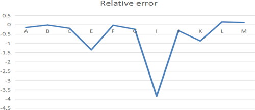
Figure 2. Relative error of A path model. Source: author's calculations.

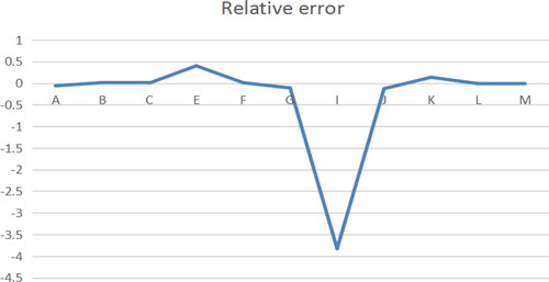
Figure 3. Relative error of B path model. Source: author's calculations.

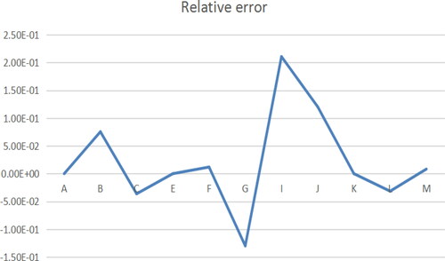
Figure 4. Relative error of C path model. Source: author's calculations.

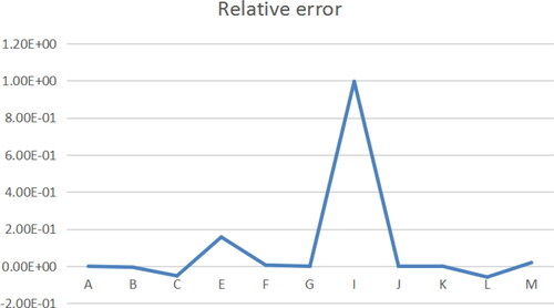
The regression estimation results of the four models show that, except for a few points, the relative error of the sample points fluctuates around zero, and the average relative errors of the three models are 0.61, 0.33, 0.021 and 0.097, respectively. The three points, namely E, L, K, are removed from the benchmark model, and the point I is removed from the A path model, which can recalculate and obtain the average relative error, namely, 0.085, 0.024, 0.021 and 0.097, respectively. The results show that the above four models have good fitting effect.

3. Analysis of industries in free trade zone

3.1. The effect of industry nature itself on tax burden

This section analyses the three causes of the difference of gross revenue between industries using the driving form of tax burden to understand the formation mechanism of the tax burden outliers, along linear and non-linear paths. It can be seen from the model (4) that the gross revenue of the industry is determined by the factors of the industry itself and control variables under national policy formulation. From the definition of the tax burden of the industry, $\theta =\raisebox{1ex}{$z_6$}\!\left/ \!\raisebox{-1ex}{$Y$}\right.,$ it can be seen that the actual tax payment (Z₆) of industry can be controlled under national policy formulation; when the tax burden of the industry is abnormal, it may be caused by the industry itself; under the adjustment of the industry itself, the tax burden of the industry will tend to be normal. It also may be caused by national policy formulation; if it is caused by the factors of the control variable, policymakers need to change their decisions to control corporate tax anomalies.

3.2. The decomposition of the tax difference in industries

The semi-parametric model of the gross revenue of the ith industry is as follows: (8) $$Y_i=a(i)x_{1i}+b(i)x_{2i}+c(i)x_{3i}+d(i)x_{4i}+e(i)x_{5i}+g_i(\mathrm{z})+{\epsilon }_i$$(8)

The semi-parametric model of the gross revenue of the jth industry is as follows: (9) $$Y_j=a(j)x_{1i}+b(j)x_{2i}+c(j)x_{3i}+d(j)x_{4i}+e(j)x_{5i}+g_j(z)+{\epsilon }_j$$(9)

The interaction between different industries under common influence (8) and (9) can obtain (10): (10) $$\begin{array}{c}{Y}_i-Y_j=(a(i)-a(j))x_{1i}+(b(i)-b(j))x_{2i}+(c(i)-c(j))x_{3i}\\ +(d(i)-d(j))x_{4i}+(e(i)-e(j))x_{5i}+g_i(\mathrm{z})-g_j(z)+{\epsilon }_i-{\epsilon }_j\end{array}$$(10)

Transform equation (10)(10) $$\begin{array}{c}{Y}_i-Y_j=(a(i)-a(j))x_{1i}+(b(i)-b(j))x_{2i}+(c(i)-c(j))x_{3i}\\ +(d(i)-d(j))x_{4i}+(e(i)-e(j))x_{5i}+g_i(\mathrm{z})-g_j(z)+{\epsilon }_i-{\epsilon }_j\end{array}$$(10) and obtain (11), $Y_i=Y_j+\sigma (ij)+{\epsilon }_{ij}$ (11) (12) $$\sigma (ij)=Y_{(i)}-Y_{(j)}-{\epsilon }_{ij}=Q_1+Q_2$$(12) (13) $$\begin{array}{c}{Q}_1=(a(i)-a(j))x_{1i}+(b(i)-b(j))x_{2i}+(c(i)-c(j))x_{3i}\\ +(d(i)-d(j))x_{4i}+(e(i)-e(j))x_{5i}\end{array}$$(13) (14) $$Q_2=g_{\mathrm{i}}(z)-g_{\mathrm{j}}(z)$$(14) (15) $${\epsilon }_{ij}={\epsilon }_i-{\epsilon }_j$$(15)

In the above equation, Q₁ is the trend of linear fluctuation, Q₂ is the trend of nonlinear fluctuation, ${\epsilon }_{ij}$ is the trend of the unobservable part, and Z is the driving variable.

According to the above equation analysis, the model can be used to calculate three parts: linear fluctuation (the influence of the nature of the industry itself), nonlinear fluctuation (the effect of driving variables) and the unobservable part.

Figure 5. Various parts of the Volatility (Benchmark model). Source: author's calculations.

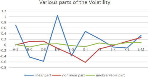
It can be seen from Figures 5–8 that the unobservable volatility is almost oscillating up and down around 0, the relative volatility is small, and the influence on dependent variables is relatively small, so it can be ignored. The volatility caused by the industry variables show a mutual alternating trend. The positive and negative values of the volatility represent the direction of the influence, and the magnitude of the volatility determines the intensity of the influence.

Figure 6. Various parts of the Volatility (A path model). Source: author's calculations.

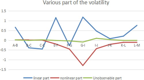
Figure 7. Various parts of the Volatility (B path model). Source: author's calculations.

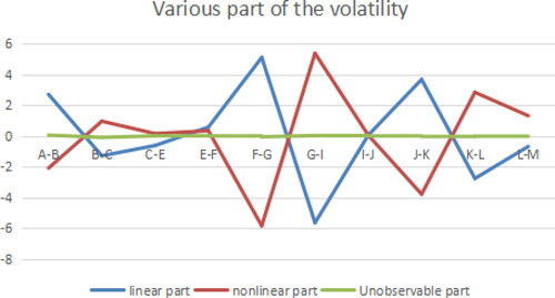
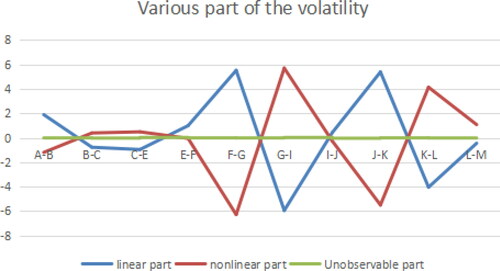
Figure 8. Various parts of the Volatility (C path model). Source: author's calculations.

Figures 9–12 describes the ratio of the volatility of each part received by each point in the four models, and specifically explains the degree of influence between industries under the influence of different factors.

Figure 9. Volatility ratio of each part (Benchmark model). Source: author's calculations.

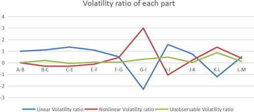
Figure 10. Volatility ratio of each part (A path model). Source: author's calculations.

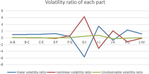
Figure 11. Volatility ratio of each part (B path model). Source: author's calculations.

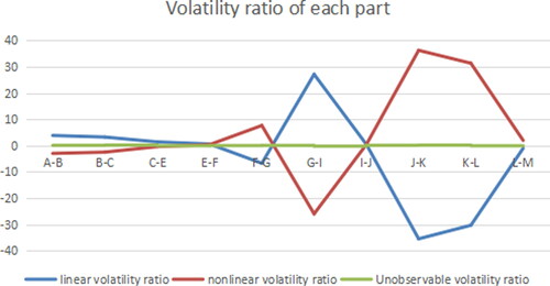
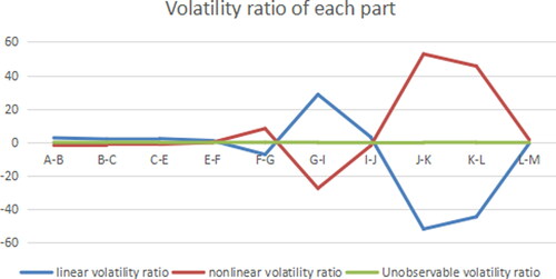
Figure 12. Volatility ratio of each part (C path model). Source: author's calculations.

According to the above analysis, the influence of error can be ignored, so the interaction between different industries is mainly reflected by linear and nonlinear parts. The linear part is that different properties, different demand and supply by different industries create the cooperation and competition among industries. The nonlinear part mainly takes into account the change of driving variables, and the sales revenue of different industries will also be affected to varying degrees.

In the previous section, different industries are ranked, and the result obtained through calculation is the influence between two adjacent industries in the model. The result changes with changes in the ranking of industries in the model. In other words, any industry can be compared with any other just by changing the position of the industry in the model. In practice, the impact between specific industries can be considered in terms of demand.

Further analysis is carried out below by determining the driving mode of mutual influence between industries.

3.3. Determination of driving mode under different paths

When judging the driving mode, the ratio of P = Q₂/Q₁ should be used to judge. If P < 1, the linear fluctuation at this time is more affected, which is trend-driven, that is to say, the influence of industry factors is greater than that of driving variables. If the tax burden of an industry fluctuates to the outlier, and it is caused simply by industry factors, it may return to a reasonable level through the interaction between the industry and the industry. On the other hand, if the ratio is greater than 1, that is, P > 1, it indicates that nonlinear fluctuation has a greater influence and is driven by oscillation. That is, the influence of driving variables is greater than that of industry factors. Through the influence between industries, the industry tax burden cannot return to a reasonable level, which needs to be driven by further increasing variables. In practice, it is controlled by policy adjustment.

Figure 13. Linear ratio of nonlinearity (Industry path). Source: Author’s computation.

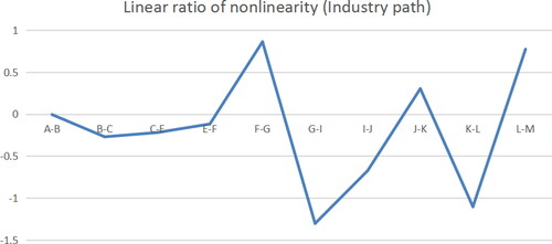
3.3.1. Industry Path

According to the abnormal tax burden industry E, G, I, K, L and Figure 13 shown above, P_(C-E), P_(F-G), and P_(J-K) are all less than 1, which indicates that the impact of industry C on industry K, industry F on industry G, industry I on industry J and industry J on industry K is linear. The industry sales of the latter can be improved by the influence of industry adjustment. P_(G-J), P_(K-L) are greater than 1, which indicates that the nonlinear fluctuation of the two industries at this time has a great influence and should wait for the decision after regression.

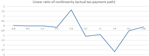
3.3.2. Actual tax payment path

By analysing the actual tax payment path, we can see in Figure 14 from the points of P > 1, including F-G, G-I, J-K, at this time, that the nonlinear fluctuations of the two industries have a greater impact and can wait for the decision after regression. From the points of P < 1 including C-E, I-J, K-L, we can see that driving form is trend driven, which can increase the industry sales of the latter through the influence between industries.

Figure 14. Linear ratio of nonlinearity (Actual tax payment path). Source: author's calculations.

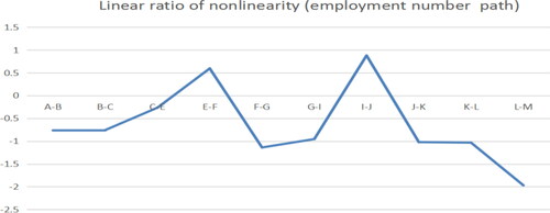
3.3.3. Employment number path

By analysing the path of employment, we can see from the point of P > 1 in Figure 15, including F-G, J-K, K-L, at this time, that the nonlinear fluctuation of the two industries has a great influence, and we can wait for decision after regression. From the the points of P < 1 including C-E, G-I, I-J, driving form is trend driven, and the industry sales of the latter can be improved through the influence between industries.

Figure 15. Linear ratio of nonlinearity (Employment number path). Source: author's calculations.

From the above analysis, it can be seen from Table 3 that the driving form of the interaction between industries under different paths will change, which means that policies of different industries need to be adjusted in order to reduce the tax burden risk more effectively.

Table 3. Driving forms of interaction between industries under different paths.

Path	C-E	F-G	G-I	I-J	J-K	K-L
Industry	P < 1	P < 1	P > 1	P < 1	P < 1	P > 1
Actual tax payment	P < 1	P > 1	P > 1	P < 1	P > 1	P < 1
Employment number	P < 1	P > 1	P < 1	P < 1	P > 1	P > 1

Source: Author’s computation.

4. Tax risk allocation of free trade zone industries

4.1. Definition of tax burden risk of free trade zone industries

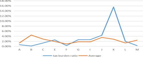
Set the industry as the horizontal axis and observe the gross revenue and actual tax payment of the selected 11 industries, as shown in Figure 16.

Figure 16. Gross revenue and actual tax payment trend. Source: author's calculations.

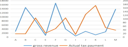
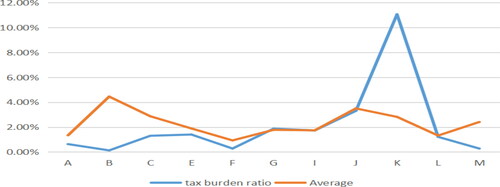
Referring to the research ideas of Xu (Xu 2010; Xu et al. 2019), this paper assumes that the enterprise’s tax burden (θ) is measured by dividing the actual tax payment amount by the total sales revenue. In this paper, the tax burden outlier of various industries in the Free Trade Zone is defined as the tax burden of this industry exceeds the average tax burden of the same industry in Zhejiang Province in the same period. The data of the average tax burden of the industry in Zhejiang Province comes from local tax authorities. The reason for the above definition is that a series of tax reduction and subsidy policies will greatly reduce the tax burden of the industry in the Free Trade Zone. Therefore, theoretically, the tax burden of the industry in the Free Trade Zone should be lower than that of the industry in Zhejiang Province in the same period.

As can be seen from Figure 17, the tax burden of six industries, namely, E, G, I, J, K, L is abnormal. Figure 16 also shows that the gross revenue of these industries is also lower than that of other industries, but the actual tax revenue has not been reduced, resulting in an excessive tax burden. The following is mainly for the above six abnormal industries to carry on the tax risk allocation.

Figure 17. Tax burden ratio and average. Source: author's calculations.

4.2. Measuring the level of tax risk

The final purpose of this paper is to reduce the tax burden risk of the industry, improve the gross revenue of the industry, and provide optional decisions for industry tax risk managers. Therefore, it is necessary to refer to certain standards to measure the quality of tax risk allocation.

According to the model (12), the following analysis can be done:

Because the error is relatively small, the impact of the unobservable part can be ignored. Therefore, we can approximate the difference of gross revenue between the ith industry and the jth industry according to the size of ${\sigma }_p(ij,z).$ The larger the ${\sigma }_p(ij,z),$ the larger the effect of the driving variable on gross revenue. Between industries, ${\sigma }_p(ij,z)-{\sigma }_0(ij)$ represents the impact of path driven variable on the gross revenue of the industry, ${\sigma }_p(ij,z_6)-{\sigma }_0(ij)$ indicates the impact of government tax payment policy on the gross revenue of the industry, ${\sigma }_p(ij,z_7)-{\sigma }_0(ij)$ represents the influence of employment policy on the gross sale revenue of industry, ${\sigma }_p(ij,z_6,z_7)-{\sigma }_0(ij)$ represents the impact of the government’s tax reduction and control of the industry scale on the industry’s gross sales revenue. The ultimate purpose of these three methods is to help various industries in the Free Trade Zone develop and grow faster, and give full play to social responsibility to maximise the economic benefits of enterprises. Since ${\sigma }_p(ij,z)-{\sigma }_0(ij)$ is an objectively calculated value, we can judge the positive or negative effects of the policy according to its value, and then choose the corresponding policy, which is most conducive to improving economic efficiency. If ${\sigma }_p(ij,z_6)-{\sigma }_0(ij),$${\sigma }_p(ij,z_7)-{\sigma }_0(ij)$ or${\sigma }_p(ij,z_6,z_7)-{\sigma }_0(ij)$ more than 0, it shows that government adjustment will not have a negative impact on the economic benefits of enterprises. If the fitting value is significantly less than 0, it indicates that there is a negative impact that cannot be ignored. So it is vital to change and adjust the policy and its intensity to further integrate and optimise social responsibility and economic benefits.

The evaluation standard for the effectiveness of risk allocation of tax burden in industry, lies in whether the actual tax revenue of enterprises can be reduced through a series of policy adjustments and ultimately promote the increase of total sales revenue of the industry, which is an important means for the sustainable development of the industry.

4.3. Tax burden allocation in industries under different paths

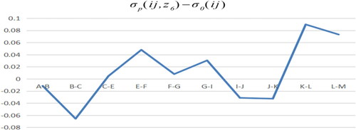
4.3.1. Actual tax payment path

In the actual tax payment path model minus the benchmark model from Figure 18, it can be seen that the negative effects of the three sample points of I-J and J-K are −0.066, −0.031 and −0.033, respectively. This shows that the influence of industry I on industry J and industry J on industry K are negative under the drive of actual tax payment. The effect of G-I, K-L, L-M is better, which is 0.030, 0.089. 0.073, respectively. It indicates that the tax policy of L, M is more reasonable for I, L, M, the tax policy of M is more reasonable for I, L, M, and the tax policy of M is more reasonable for I, L, M.

Figure 18. A path model minus benchmark model. Source: author's calculations.

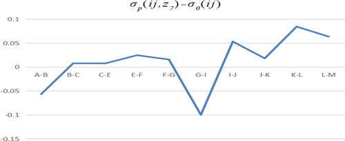
4.3.2. Employment number path

With B path model minus benchmark model, it can be seen from Figure 19 that the negative effect of G-I sample is large. Under the action of employment policy, the influence of industry G on industry I is negative. The positive effect of sample points of I-J, K-L is relatively large, which indicates that the adjustment effect of government employment policy is ideal for industry J, L.

Figure 19. B path model minus benchmark model. Source: author's calculations.

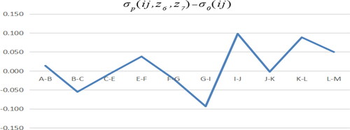
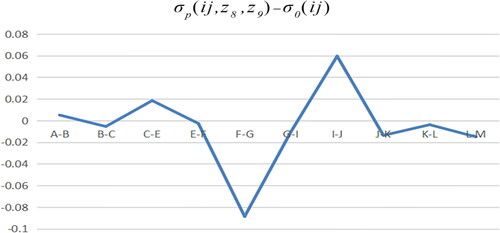
4.3.3. The path of the interaction between the actual tax payment and the employment number

From the results of C path model minus the benchmark model shown in Figure 20, it can be seen that under the action of the two policies, the influence of industry I on industry J and industry K on industry L is positive, industry G has great negative effect on industry I, and the role of tax burden to other industries is not obvious.

Figure 20. C path model minus benchmark model. Source: author's calculations.

According to the results of the above three path models, the five abnormal industries are summarised and compared, and Table 4 is obtained.

Table 4. Comparison between different path models and benchmark models.

	C-E	F-G	G-I	I-J	J-K	K-L
${\sigma }_p(ij,z_6)-{\sigma }_0(ij)$	0.005	0.008	0.030	−0.031	−0.033	0.090
${\sigma }_p(ij,z_7)-{\sigma }_0(ij)$	0.007	0.016	−0.100	0.053	0.018	0.084
${\sigma }_p(ij,z_6,z_7)-{\sigma }_0(ij)$	0.008	−0.021	−0.093	0.098	−0.02	0.088

Source: author's calculations.

As can be seen from Table 4, in order to reduce the impact of negative effects, different path models are required for analysis, that is, different policies are required in practice. After adopting the tax reduction policy, industry G is the most helpful to industry I and industry K is most helpful to industry L in increasing turnover. After adopting active industry employment policies, industry C is most helpful to industry E, industry F to industry G, industry J to industry K to increase turnover. At the same time, after adopting tax reduction policy and active industry employment policy, I industry is the most helpful to J industry.

4.4. Optimisation of tax burden risk allocation in different industries

From the above analysis, it can be seen that the effect of industry tax risk allocation under different policies is different. Now we adjusted different policies for industries with high tax burden in the Free Trade Zone. In industry E, the average tax cut was 100,000 yuan and employment increased by 5. In industry G, the average tax cut was 300,000 yuan and employment increased by 10. The average tax cut in industry I is 50,000 yuan, with 5 people gaining employment. The average tax cut in industry J is 300,000 yuan, with 5 people gaining employment. The average tax cut in industry K is 500,000 yuan, with 10 people gaining employment. The average tax cut in industry L is 200,000 yuan, with 5 people gaining employment. As shown in Table 5.

Table 5. Adjustment of actual tax amount and employment scale.

Industry	Code	Reduce taxes	Expand the scale of employment
Agriculture, forestry, animal husbandry and fishery	A
The mining industry	B
Manufacturing	C
Construction industry	E	10	5
Wholesale and retail	F
Transportation, warehousing and postal industry	G	30	10
Information transmission, software and information technology services	I	5	5
Financial industry	J	30	5
The real estate industry	K	50	10
Leasing and business services	L	20	5
Scientific research and technological services	M

Source: author's calculations.

Under the effect of policy adjustment, the tax burden of each industry has been greatly reduced, as shown in Figure 21. In addition to industry K, the tax burden of other industries has been reduced below the average level of the whole province, and the tax burden pressure of K industry has obviously been reduced as well.

Figure 21. Adjusted tax burden ratio and average. Source: author's calculations.

The actual tax payment (Z₈) and employment number (Z₉) of the new nonlinear variables are obtained after the change of tax payment and industry employment number, and Figures 22–24 are obtained by calculation.

Figure 22. Adjusted A path model minus benchmark model. Source: author's calculations.

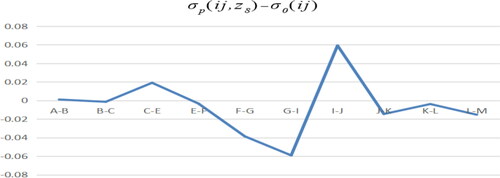
Figure 23. Adjusted B path model minus benchmark model. Source: author's calculations.

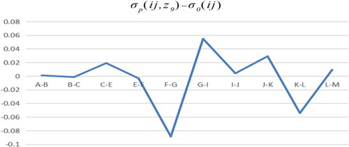
Figure 24. Adjusted C path model minus benchmark model. Source: author's calculations.

We compare Figures 18–20 with Figures 22–24 to observe the effect of the above (Table 5) adjustment.

When industry E reduces tax and expands employment at the same time, industry C makes a positive contribution to industry E’s turnover. For industry G, whether its tax reduction or industry expansion, industry F has a negative effect on the increase of industry G^’s turnover. For industry I, with industry expansion or tax reduction and expansion at the same time, industry G has a positive effect on its turnover increase. For industry J, tax reduction policy is adopted directly, and industry I plays the largest role in increasing its turnover. For industry K, positive employment policies should be adopted, and industry J has the largest effect on the increase of its turnover. For industry L, the adjustment range in Table 4 shows that industry K is unfavourable to the business improvement of industry L, and the policy strength should be further improved.

Generally speaking, in the process of actively promoting tax reduction in various industries in the Free Trade Zone, not all industries will experience improved economic benefits, so it is necessary to adopt other policy means to ensure that the economic benefits of enterprises do not decline. This paper refers to the adoption of appropriate employment policies to achieve the best effect of tax risk allocation in free trade area industries. The key lies in accurately grasping the intensity of tax reduction in different industries and accurately regulating the size of the industry. The ability of each industry to deal with tax risk is different, and different policies should be implemented for different industries (Shen, 2014).

5. Conclusion

The establishment of Free Trade Zones is a new model for China’s development. Free Trade Zones affect the transformation and upgrading of regional industrial structure through investment structure, import trade structure, export trade structure, economic growth and consumer demand. Zhejiang Province promotes technological innovation through the establishment of a pilot Free Trade Zone. The establishment of the tax system of the Free Trade Zone and the exploration of a new tax system with international competitiveness are important guarantees for the rapid and sound development of the pilot Free Trade Zone, which are of great significance to the sustainable development of China’s economy. Our purpose in writing this paper is to provide an alternative strategy for tax policy improvement so that the enterprise tax burden in the pilot Free Trade Zone can be within a range, that is, the enterprise tax burden can just promote the enterprise development.

The paper found six industries with abnormal tax burdens in China (Zhejiang) Pilot Free Trade Zone in 2017. According to the results of the analysis, the tax burden anomaly industry in China (Zhejiang) Pilot Free Trade Zone in 2017 is mainly concentrated in the tertiary industry, and there is a certain gap of tax burden among different industries.

By constructing the semi-parameter time-varying model and adding different driving variables to get the path model, the tax risk allocation of 3,585 enterprises in China (Zhejiang) Pilot Free Trade Zone in 2017 is calculated. It is found that the tax burden pf each industry, due to the different natural attributes, has a different degree of fluctuation. Under the individual and joint driving of the two control variables of actual tax payment and employment number, the tax burden shock of different industries is obviously different. In the improvement of tax policies, the tax burden among different enterprises will also have an impact. Moreover, driven by the two control variables of actual tax payment and the number of employees, respectively and jointly, there are significant differences in the degree of mutual influence among different industries, which means that different policies need to be adopted for different industries to achieve the purpose of not only increasing industry sales but also reducing industry tax burden risk.

Finally, the paper discusses three ways of tax risk allocation in the Free Trade Zone industry and optimises the level of tax risk allocation in the industry with excessive tax burden in the Free Trade Zone through policy adjustment. From the perspective of optimisation effect, the adjustment of tax revenue and industry scale has certain positive effects on the allocation of industry tax burden risk, and the key lies in the intensity and pertinence of relevant policies.

The research results of this paper provide the basis for the government to take correct decisions on the development of various industries in the Free Trade Zone, that is, to adopt different tax policies for different industries, supplemented by appropriate employment policies, in order to improve the risk allocation level of industry tax burden, promote the sustainable development of the economy in the Free Trade Zone and fulfill the necessary social responsibilities.

Acknowledgments

We would like to express great appreciation to China (Zhejiang) Pilot Free Trade Zone research institute for its support of our research.

Disclosure statement

The author declares that there is no conflict of interest.

Notes

1 For the estimation of the parameters of this model, please refer to the monograph ‘non-parametric analysis of taxation and its policy effects’ by Shen (2014).

2 From the perspective of endogenous variables and exogenous variables, we believe that the enterprise tax burden and the proportion of disabled people in employment are exogenous variables controlled by national policies.

References

- Chek, D., & Hao, Z. (2003). Effective tax rates and the ‘industrial policy’ hypothesis: Evidence from Malaysia. Journal of International Accounting, Auditing and Taxation, 12(1), 45–62.
- Civera, A., Donina, D., Meoli, M., & Vismara, S. (2019). Fostering the creation of academic spinoffs: does the international mobility of the academic leader matter? International Entrepreneurship and Management Journal, 16(2), 439–465.
- Dileo, I., & García Pereiro, T. (2019). Assessing the impact of individual and context factors on the entrepreneurial process. A cross-country multilevel approach. International Entrepreneurship and Management Journal, 15(4), 1393–1441. https://doi.org/https://doi.org/10.1007/s11365-018-0528-1
- Fang, H., Yu, L., Hong, Y., & Zhang, J. (2019). Tax burden, regulations and development of service sector in China. Emerging Markets Finance and Trade, 55(3), 477–495. https://doi.org/https://doi.org/10.1080/1540496X.2018.1469001
- Hall, P., Li, Q., & Racine, J. S. (2007). Nonparametric estimation of regression functions in the presence of irrelevant regressors. Review of Economics and Statistics, 89(4), 784–789. https://doi.org/https://doi.org/10.1162/rest.89.4.784
- Haverals, J. (2007). IAS/IFRS in Belgium quantitative analysis of the impact on the tax burden of companies. Journal of International Accounting, Auditing and Taxation, 16(1), 69–89. https://doi.org/https://doi.org/10.1016/j.intaccaudtax.2007.01.005
- Jiang, M. Y. (2011). The effects of the extending VAT tax base reform on sector’s tax burden. Journal of Central University of Finance & Economics, 2, 11–16. (In Chinese)
- Ren, A., & Qian, Y. (2017). Asymmetric effects of fiscal policy on industrial structure optimisation in China. East China Economic Management, 31(4), 111–120. (In Chinese)
- Shen, Z. Y. (2014). Nonparametric analysis of taxation and its policy effects. Economic Science Press.
- Wang, H. C., & Liu, S. H. (2017). Tax competition in industries based on the relative tax burden. Journal of Chinese Academy of Governance, 3, 87–91. (In Chinese)
- Xu, B. (2010). Path converged design application to production efficiency of FDI in regions. Economic Research Journal, 45(02), 44–54. (In Chinese)
- Xu, B., Li, L., Liang, Y., & Rahman, M. U. (2019). Measuring risk allocation of tax burden for small and micro enterprises. Sustainability (Switzerland), 11(3), 741. https://doi.org/https://doi.org/10.3390/su11030741
- Yu, W. T., Zhou, X. L., & You, W. H. (2017). Taxation reduction, firm size heterogeneity and productivity growth: Based on the data from the creative sectors in Jiangsu Province. Journal of Nanjing University of Aeronautics and Astronautics, 19(04), 18–24. (In Chinese)