Investment decision making based on the probabilistic hesitant financial data: model and empirical study

Abstract

This paper proposes a portfolio selection model from the perspective of probabilistic hesitant financial data (PHFD). PHFD can be interpreted as the new form of information presentation that is obtained by transforming real financial data into probabilistic hesitant fuzzy elements. Based on the above data and model, we can derive the optimal investment ratios and give suggestions for investors. Specifically, this paper first develops a transformation algorithm to transform the general share returns into PHFD. The transformed data can directly show all the returns and their occurrence probabilities. Then, the portfolio selection and risk portfolio selection models based on PHFD, namely the probabilistic hesitant portfolio selection (PHPS) model and the risk probabilistic hesitant portfolio selection (RPHPS) model, are proposed. Furthermore, the investment decision-making methods are provided to show their practical application in financial markets. It is pointed out that the PHPS model for general investors is constructed based on the maximum-score or minimum-deviation principles to get the optimal investment ratios, and the RPHPS model provides the optimal investment ratios for three types of risk investors with the aim of obtaining the maximum return or taking the minimum risk. Finally, an empirical study based on the real data of China’s stock markets is shown in detail. The results verify the effectiveness and practicability of the proposed methods.

Keywords:

• Probabilistic hesitant financial data
• portfolio selection
• investment decision making
• optimal investment ratio
• China’s stock market

SUBJECT CLASSIFICATION CODES:

• C10
• G10
• G24

1. Introduction

In this paper, we propose a portfolio selection model from the perspective of probabilistic hesitant financial data (PHFD). It is a new form of information presentation that is obtained by transforming real financial data into probabilistic hesitant fuzzy elements (PHFE). Note that PHFD are presented by returns and their occurrence probabilities based on real financial data. As we know, the traditional model (Markowitz, 1952) is calculated based on the mean and variance of returns. Obviously, these two portfolio selection models and their optimal results are different. How to choose the better one from these two models? This depends on the investors’ subjective evaluation. If an investor prefers to the return and risk of share represented by the mean and variance values, then the traditional Markowitz model is better. If an investor focuses on the returns and their occurrence probability, then the new model is better. Therefore, PHFD, the new portfolio selection model and their empirical study are the main contributions of this paper.

In this paper, the empirical study focuses on China’s stock markets because of the price restriction policy. Thus, the share returns can clearly show the desired characters of PHFD. For example, according to the price restriction policy, the share returns in China’s stock markets are restricted to the interval $[-10\%,\mathrm{ }10\%].$ Thus, investors focus on the return results with two decimal places, namely $\{-0.10,\mathrm{ }-0.09,\mathrm{ }\cdots ,\mathrm{ }0.09,\mathrm{ }0.10\}$ because many data shown by the financial marks remain two decimal places. Based on this, for a time series of share returns, we can transform them into PHFD with corresponding occurrence probabilities. Obviously, the transformed data with corresponding occurrence probabilities are consistent with PHFE, and we can name it as PHFD. This provides a feasible theoretical foundation to express the real share returns of financial products in the form of probabilistic hesitant fuzzy set (PHFS). Then, this paper further researches the portfolio selection models under the PHFD environment to obtain the optimal investment ratios and make an investment decision. Based on the obtained optimal results, which are different from those calculated by the traditional methods, we can provide some investment suggestions for investors. It is pointed out that the original data used to construct models are the same in the traditional methods and the proposed ones. To achieve these aims, we review the related methods as follows:

The portfolio model was proposed by Markowitz (1952) which is well-known in the investment decision-making field. This model has been extended and applied in many ways, especially on the following three aspects. First, to develop the portfolio selection approach, some new models have been proposed such as the insurance and investment portfolio model (Li, 1995), the quadratic portfolio model (Castellacci & Siclari, 2003), the robust multi-period portfolio model (Liu et al., 2015), the scenario-based portfolio model (Vilkkumaa et al., 2018), and the sparse chance constrained portfolio selection model (Chen et al., 2020). The extended forms and models can deal with different types of portfolio selection issues according to the different aims. Second, to optimize the existing portfolio selection methods, some improved models have been presented, such as the mean absolute deviation portfolio model (Simaan, 1997), the Bayesian framework portfolio model (Pástor, 2000), the mean-VaR portfolio model (Alexander & Baptista, 2002), the chance constrained portfolio model (Abdelaziz et al., 2007), the constrained fuzzy analytic hierarchy portfolio model (Nguyen & Gordon-Brown, 2012), the risk-return portfolio model (Brandtner et al., 2018), and the mean-risk portfolio model (Mehralizade et al., 2020). Third, to deal with different real problems, some new models have been designed. These problems include the institutional procedures for short selling (Kwan, 1997), the independent possibilistic information (Inuiguchi & Tanino, 2000), the robust estimation (Demiguel & Nogales, 2009), the concave price impact (Ma et al., 2013), the uncertain environment impact (Li et al., 2018), and the limited market liquidity (Ha & Zhang, 2020). Obviously, the traditional portfolio models have been further developed in the above literature. In this paper, we further develop the traditional models from the environmental perspective, namely, the PHFD environment. Considering this special environment, the proposed models are innovative and can be used to deal with different investment-decision issues.

We can find that the above portfolio selection models tend to use accurate numbers but overlook the uncertainty of data. Therefore, many uncertain portfolio selection models based on fuzzy environments have been proposed, such as the fuzzy dynamic portfolio selection model (Östermark, 1996), the fuzzy chance-constrained portfolio selection model (Huang, 2006), the cardinality constrained fuzzy portfolio selection model (Bermúdez et al., 2012), the new bi-objective fuzzy portfolio selection model (Kar et al., 2019), and the fuzzy multi-objective portfolio selection model (Chen et al., 2020). In these models, the uncertainty of data is addressed by different fuzzy sets (Zadeh, 1965). Moreover, by applying them to practical portfolio selection issues, a series of fuzzy portfolio models have been successfully used in various fields such as strategic management (Pap et al., 2000), the stock market analysis (Teresa et al., 2004), the security risk calculation (Huang, 2011), the large-scale rooftop PV project investment (Wu et al., 2018), and the efficiency evaluation (Gupta et al., 2020). Compared with the portfolio selection models constructed based on accurate data, these fuzzy portfolio selection models are mainly used in uncertain and fuzzy environments. Therefore, they are introduced as the theoretical foundation of this paper due to their significant contributions to the portfolio selection theory.

Also, we can find that the above fuzzy portfolio models are mainly constructed based on fuzzy sets. Then, a direct method to further develop these methods is to introduce new and different fuzzy sets such as the intuitionistic fuzzy set (Atanassov, 1986), the convex fuzzy set (Sarkar, 1996), the type-2 fuzzy set (Karnik & Mendel, 2001), the interval type-2 fuzzy set (Mendel & Wu, 2007), the interval-valued fuzzy set (Yang et al., 2009), the hesitant fuzzy set (HFS) (Torra & Narukawa, 2009), the probabilistic rough fuzzy set (Sun et al., 2014), the interval-valued intuitionistic fuzzy set (Li, 2018), and the probabilistic linguistic q-rung orthopair fuzzy set (Liu & Huang, 2020). Then, many developed fuzzy portfolio selecition models have been proposed, such as the fuzzy portfolio model (Watada, 2001), the trapezoidal LR-fuzzy portfolio selection (Vercher et al., 2007), the intuitionistic fuzzy optimal portfolio selection (Chen et al., 2011), the interactive fuzzy efficient portfolio selection (Rebiasz, 2013), the interval type-2 fuzzy portfolio optimization (Pai, 2017), the hesitant fuzzy portfolio selection (Zhou & Xu, 2018), and the dual hesitant fuzzy portfolio selection (Li & Deng, 2020). Thus, the traditional portfolio selection model has been extensively studied in diverse fuzzy environments. Similar to the above fuzzy portfolio selection models, we develop a new model by introducing the PHFD environment. Unlike the above fuzzy portfolio selection models, PHFD come from the real financial data which is also its prominent advantage.

As aforementioned, we mainly focus on two types of portfolio selection models under the PHFD environment to help investors make investment decisions from different perspectives. As a result, this paper has three main contributions to the literature in economics and finance as well as practical implications: (1) This paper designs a transformation algorithm to obtain PHFD based on real financial data. The desired advantage of PHFD is to show the returns and their occurrence probabilities simultaneously. (2) This paper proposes the probabilistic hesitant portfolio selection (PHPS) model and the risk probabilistic hesitant portfolio (RPHP) model for general investors and risk investors under the PHFD environment, respectively. (3) This paper gives an empirical study in detail and applies the proposed models to four stocks in the biological vaccine concept sector of China’s stock markets. It illustrates an investment decision-making process that is different from which using traditional methods and they can be practically used by investors.

To achieve the above aims, the rest of this paper is constructed as follows: we introduce the basic definitions and operations of HFS and PHFS, then develop the transformation algorithm and give the definition of PHFD in Section 2. In Section 3, we propose the PHPS models to get the optimal investment ratios for general investors. Based on which, Section 4 further develops the RPHPS models to obtain the optimal investment ratios for three types of risk investors. Furthermore, an empirical study is given to fully show the proposed methods in Section 5. Finally, the conclusion can be seen in Section 6.

2. Probabilistic hesitant financial data and its acquisition

In this section, we introduce the basic definitions of HFS (Torra & Narukawa, 2009) and PHFS (Xu & Zhou, 2017), which are the theoretical foundations for further methods. Then, we demonstrate the transformation algorithm and definition of PHFD to change the share returns of financial products into PHFD. After that, the real acquisition of PHFD is realized.

2.1. HFS and PHFS

It can be found that PHFS is an extended form of HFS. Both of them use a set of possible values to express the subjective evaluation information given by decision makers. However, they are obviously unlike in the description of occurrence probabilities using different possible values. For more details, we present them as follows:

Definition 1.

(Torra & Narukawa, 2009). Let $X$ be an invariant set, we define HFS on $X$ according to the function $h,$ so that when it is applied to $X,$ it returns a subset of [0,1].

Xia and Xu (2011) described HFS with a mathematical symbol $E=\{<x,h_E(x)>|x\in X\},$ where $h_E(x)$ is a set of values in [0,1], representing the possible membership degrees of element $x\in X$ to the set $E,$ and they called $h=h_E(x)$ a hesitant fuzzy element (HFE).

We can find that the occurrence probabilities of all possible values in HFE are equal. Then, Xu and Zhou (2017) developed PHFS and PHFE, in which the occurrence probabilities of all possible values are unequal. The basic definitions and operations are presented below:

Definition 2.

(Xu & Zhou, 2017). Let $R$ be an invariant set, then a PHFS on $R$ is described with a mathematical symbol:

(1) $$H_P=\{\overline{h}({\gamma }_t{}^{<p_t>})|{\gamma }_t,p_t\}$$(1)

where $\overline{h}({\gamma }_t{}^{<p_t>})$ is a set of some elements ${\gamma }_t{}^{<p_t>}$ and denotes the probabilistic hesitant fuzzy information of $H_P,$ ${\gamma }_t\in R,$ $0\le {\gamma }_t\le 1,$ $t=1,2,\dots ,\#\overline{h},$ where $\#\overline{h}$ is the number of possible elements in $\overline{h}({\gamma }_t{}^{<p_t>}),$ $p_t\in [0,1]$ is the occurrence probability of ${\gamma }_t,$ and ${\sum }_{t=1}^{\#\overline{h}}{p}_t=1.$

Further, the score function $\mathrm{S}(\overline{h})$ and the deviation function $\mathrm{D}(\overline{h})$ are given to compare the different PHFEs. We have $\mathrm{S}(\overline{h})={\sum }_{t=1}^{\#\overline{h}}{\gamma }_t{p}_t$ and $\mathrm{D}(\overline{h})=\sqrt{{\sum }_{t=1}^{\#\overline{h}}{({\gamma }_t-\mathrm{S}(\overline{h}))}^2{p}_t}.$

Let two PHFEs be $\overline{h}({\gamma }_t{}^{<p_t>})$ and ${\overline{h}}^{\prime }({\gamma }_{t^{\prime }}{}^{<p_{t^{\prime }}>}),$ the basic operations can be presented as

$\overline{h}\oplus {\overline{h}}^{\prime }=\underset{t=1,2,\dots ,\#\overline{h},t^{\prime }=1,2,\dots ,\#{\overline{h}}^{\prime }}{\cup }\left\{{({\gamma }_t+{\gamma }_{t^{\prime }}-{\gamma }_t{\gamma }_{t^{\prime }})}^{<p_t{p}_{t^{\prime }}>}\right\},$ and $$\lambda \overline{h}=\underset{t=1,2,\dots ,\#\overline{h}}{\cup }\left\{{(1-{(1-{\gamma }_t)}^{\lambda })}^{<p_t>}\right\}.$$ where $t=1,2,\dots ,\#\overline{h},$ $t^{\prime }=1,2,\dots ,\#{\overline{h}}^{\prime },$ ${\sum }_{t=1}^{\#\overline{h}}{p}_t=1,$ ${\sum }_{t^{\prime }=1}^{\#\overline{h}}{p}_{t^{\prime }}=1,$ and $\lambda >0.$

It can be found that PHFS is more comprehensive than HFS. Therefore, we mainly study the share return under the probabilistic hesitant fuzzy environment then propose the transformation algorithm and the definition of PHFD in the next section.

2.2. Transformation algorithm and definition of PHFD

It is pointed out that the following algorithm is given based on the real situations in China’s stock markets and the price restriction policy. For different financial markets and price policies, we can similarly derive the models and conclusions.

Algorithm 1 is given to transform real financial data, namely share returns, into PHFD.

Algorithm 1. Transform the share returns into PHFD.

• Step 1: Obtain the share prices $\mathrm{ }{S}_k\mathrm{ }(k=1,2,\dots ,n)$ and calculate their returns, which can be presented as $H_k=\frac{S_k-S_{k-1}}{S_{k-1}}.$ Here, we have $H_k\in [-0.1,0.1]$ according to the price restriction policy in China’s stock market.

• Step 2: Calculate ${\dot{H}}_k$ according to ${\dot{H}}_k=0.5(H_k+0.1)$ where $H_k\in [-0.1,0.1].$ Thus, we can change the negative values in $\mathrm{ }{H}_k$ into the positive values and make sure that ${\dot{H}}_k\in [0,0.1].$

• Step 3: Transform ${\dot{H}}_k$ into ${\ddot{H}}_k$ based on ${\ddot{H}}_k=[100{\dot{H}}_k]\mathrm{ }\times {10}^{-2}\mathrm{ }(k=1,2,\dots ,n),$ where $[\cdot ]$ is the integer operation. Thus, the ${\ddot{H}}_k$ only keep two decimal places.

• Step 4: Collect the same values in $\ddot{H}=\underset{k=1,2,\dots ,n}{\cup }\left\{{\ddot{H}}_k\right\}$ and present as $\widehat{h}=\underset{t=1,2,\dots ,\#h}{\cup }\left\{{\gamma }_t\right\}.$

• Step 5: Compute the occurrence probability ${\vartheta }_t$ of ${\gamma }_t^{}$ in $\widehat{h}=\underset{t=1,2,\dots ,\#h}{\cup }\left\{{\gamma }_t\right\}$ based on $\ddot{H}=\underset{k=1,2,\dots ,n}{\cup }\left\{{\ddot{H}}_k\right\},$ and then we can get the corresponding PHFD $h=\underset{t=1,2,\dots ,\#h}{\cup }\left\{{\gamma }_t^{<{\vartheta }_t>}\right\},$ where ${\gamma }_t$ $\mathrm{ }\mathrm{(}t=1,2,\dots ,\#h\mathrm{)}$ are the different elements in $h,$ ${\vartheta }_t$ is the occurrence probability of ${\gamma }_t,$ and ${\sum }_{t=1}^{\#h}{\vartheta }_t=1.$

End

To show the specific transformation process by using the above transformation algorithm, a simple example is illustrated as follows:

Example 1.

For a stock $S,$ we obtain its share prices for 11 consecutive trading days shown in Step 1. To transform these share prices to PHFD, Algorithm 1 is used below:

• Step 1: Obtain 11 share prices $\mathrm{ }{S}_0=26.07,$ $\mathrm{ }{S}_1=26.32,$ $S_2=28.25,$ $S_3=28.58,\mathrm{ }\cdots ,$ $S_8=31.00,$ $S_9=30.32,$ and $S_{10}=29.30,$ then get their share returns $H_1=0.0096,$ $H_2=0.0733,$ $H_3=0.0117,$ $\cdots ,$ $H_8=0.0794,$ $H_9=-0.0219,$ and $H_{10}=-0.0336.$

• Step 2: Calculate ${\dot{H}}_k$ according to ${\dot{H}}_k=0.5(H_k+0.1).$ Then, we have ${\dot{H}}_1=0.0548,\mathrm{ }$ ${\dot{H}}_2=0.0867,$ ${\dot{H}}_3=0.0558,$ $\cdots ,$ ${\dot{H}}_8=0.0897,$ ${\dot{H}}_9=0.0390,$ and ${\dot{H}}_{10}=0.0332.$

• Step 3: Transform ${\dot{H}}_k$ into ${\ddot{H}}_k$ based on ${\ddot{H}}_k=[100{\dot{H}}_k]\mathrm{ }\times {10}^{-2}\mathrm{ }(k=1,2,\dots ,n),$ then we can get ${\ddot{H}}_1=0.05,\mathrm{ }{\ddot{H}}_2=0.08,\mathrm{ }{\ddot{H}}_3=0.05,\mathrm{ }\cdots ,\mathrm{ }{\ddot{H}}_8=0.08,\mathrm{ }{\ddot{H}}_9=0.03,\mathrm{ }{\ddot{H}}_{10}=0.03.$

• Step 4: Collect the same values in $\ddot{H}=\{0.05,\mathrm{ }0.08,\mathrm{ }0.05,\mathrm{ }\cdots ,\mathrm{ }0.08,\mathrm{ }0.03,\mathrm{ }0.03\}$ and show them in a HFE $\widehat{h}=\{0.03,\mathrm{ }0.05,\mathrm{ }0.08\}.$

• Step 5: Derive the occurrence probability ${\vartheta }_t$ of ${\gamma }_t^{}$ in $\widehat{h}=\{0.03,\mathrm{ }0.05,\mathrm{ }0.08\},$ then we can obtain the corresponding PHFD $h=\{{0.03}^{<0.3>},{0.05}^{<0.5>},{0.08}^{<0.2>}\}.$

After the above steps, we can change the share prices into PHFD.

This calculation process also reflects the feasibility of the proposed transformation algorithm. Based on the above calculations and analysis, we define PHFD as follows:

Definition 3.

Let $\mathrm{ }{S}_k$ $(k=1,2,\dots ,n)$ be the share prices of a financial product in $n$ consecutive trading days, then the corresponding PHFD are defined as $h=\underset{t=1,2,\dots ,\#h}{\cup }\left\{{\gamma }_t^{<{\vartheta }_t>}\right\},$ where ${\gamma }_t^{<{\vartheta }_t>}$ is the $t$^th share return with the occurrence probability ${\vartheta }_t,$ $h=\underset{t=1,2,\dots ,\#h}{\cup }\left\{{\gamma }_t^{<{\vartheta }_t>}\right\}$ is obtained based on Algorithm 1, ${\gamma }_t\in [0,0.1],$ ${\vartheta }_t\in [0,1],$ ${\sum }_{t=1}^{\#h}{\vartheta }_t=1\mathrm{ },$ $\#h$ is the number of possible elements in $h,$ $\mathrm{ }{S}_k>0,$ and $i=1,2,\dots ,m.$

From Definition 3, we can find that PHFD are similar to PHFE; however, they are different in the obtaining process. PHFD are got based on the real finance data and PHFE is given by the decision makers based on the subjective evaluation.

In this section, we first introduce HFS and PHFS. Then, the transformation algorithm, namely Algorithm 1, is proposed to change the real financial data into PHFD. After that, we formally provide Definition 3 to describe PHFD in detail. Therefore, we can derive the two following conclusions:

1. PHFD can show the share returns and their occurrence probabilities. Meanwhile, it also owns certain and uncertain characters as it is similar to PHFE which is an emerging fuzzy number.

2. The given Algorithm 1 can transform share returns into PHFD directly. In the next section, we further develop the portfolio selection models and their investment decision-making process based on the proposed PHFD.

3. Probability hesitant portfolio selection models in the PHFD environmnet

In this section, we focus on the portfolio selection models in the PHFD environment to obtain the optimal results. Thus, investment suggestions can be given to investors accordingly. Similar to the hesitant fuzzy portfolio selection models proposed by Zhou and Xu (2018), we first develop two basic PHPS models based on the maximum-score objective and the minimum-deviation objective. Then, they are further developed by introducing the investors’ risk appetite.

To construct the PHPS models, the general application scenario is set up as follows: An investor plans to invest a sum of money in $m$ financial products $\{x_1,x_2,\dots ,x_m\}.$ To do this, he/she gets their share prices in $n+1$ consecutive trading days which are presented as $S_{i0},\mathrm{ }{S}_{i1},\mathrm{ }{S}_{i2},\mathrm{ }\cdots ,\mathrm{ }{S}_{in}$ $\mathrm{(}i=1,2,\dots ,m).$ To derive the optimal investment ratios of $m$ financial products based on the objective of the maximize return or the minimize risk, two basic PHPS models are proposed as follows:

Model 1: (2) $$\begin{array}{c}U1(W)=\max \mathrm{S}\left\{\underset{\begin{array}{c}{t}_1=1,2,\dots ,\#h_1,\mathrm{ }{t}_2=1,2,\dots ,\#h_2,\\ \cdots ,\mathrm{ }{t}_m=1,2,\dots ,\#h_m\end{array}}{\cup }\left\{1-{\prod }_{i=1}^m{(0.1-{\gamma }_{i{t}_i}^{<{\vartheta }_{i{t}_i}>})}^{w_i}\right\}\right\}\\ \mathit{\text{s}}.t.\{\begin{array}{c}{\oplus }_{i=1}^m{w}_i{h}_i({\gamma }_{i{t}_i}^{<{\vartheta }_{i{t}_i}>})=\underset{\begin{array}{c}{t}_1=1,2,\dots ,\#h_1,\mathrm{ }{t}_2=1,2,\dots ,\#h_2,\\ \cdots ,\mathrm{ }{t}_m=1,2,\dots ,\#h_m\end{array}}{\cup }\left\{1-{\prod }_{i=1}^m{(0.1-{\gamma }_{i{t}_i}^{<{\vartheta }_{i{t}_i}>})}^{w_i}\right\}\hfill \\ {\vartheta }_{i{t}_i}=\frac{\#{\gamma }_{i{t}_i}}{{\sum }_{t_i=1}^{\#h_i}\#{\gamma }_{i{t}_i}}\\ {\sum }_{i=1}^m{w}_i=1,w_i\ge 0,i=1,2,\dots ,m.\end{array}\end{array},$$(2) where $\mathrm{S}\{\cdot \}$ is the score function of PHFD, $h_i=\underset{t_i=1,2,\dots ,\#h_i}{\cup }\left\{{\gamma }_{i{t}_i}^{<{\vartheta }_{i{t}_i}>}\right\}$ is PHFD of $i$^th financial product $x_i,$ ${\gamma }_{i{t}_i}^{<{\vartheta }_{i{t}_i}>}$ is the $t_i$^th return of $x_i$ with an occurrence probability of ${\vartheta }_{i{t}_i},$ ${\gamma }_{i{t}_i}\in [0,0.1],$ ${\vartheta }_{i{t}_i}\in [0,1],$ ${\sum }_{t_i=1}^{\#h_i}{\vartheta }_{i{t}_i}=1\mathrm{ },$ $\#h_i$ is the number of the same value of $h_i,$ $w_i$ is the investment ratio for the $i$^th financial product, and $i=1,2,\dots ,m.$

Model 2: (3) $$\begin{array}{c}U2(W)=\min \mathrm{D}\left\{\underset{\begin{array}{c}{t}_1=1,2,\dots ,\#h_1,\mathrm{ }{t}_2=1,2,\dots ,\#h_2,\\ \cdots ,\mathrm{ }{t}_m=1,2,\dots ,\#h_m\end{array}}{\cup }\left\{1-{\prod }_{i=1}^m{(0.1-{\gamma }_{i{t}_i}^{<{\vartheta }_{i{t}_i}>})}^{w_i}\right\}\right\}\end{array}\mathit{\text{s}}.t.\{\begin{array}{c}{\oplus }_{i=1}^m{w}_i{h}_i({\gamma }_{i{t}_i}^{<{\vartheta }_{i{t}_i}>})=\underset{\begin{array}{c}{t}_1=1,2,\dots ,\#h_1,\mathrm{ }{t}_2=1,2,\dots ,\#h_2,\\ \cdots ,\mathrm{ }{t}_m=1,2,\dots ,\#h_m\end{array}}{\cup }\{1-{\prod }_{i=1}^m{(0.1-{\gamma }_{i{t}_i}^{<{\vartheta }_{i{t}_i}>})}^{w_i}\}\hfill \\ {\vartheta }_{i{t}_i}=\frac{\#{\gamma }_{i{t}_i}}{{\sum }_{t_i=1}^{\#h_i}\#{\gamma }_{i{t}_i}}\\ {\sum }_{i=1}^m{w}_i=1,w_i\ge 0,i=1,2,\dots ,m.\end{array},$$(3) where $\mathrm{D}\{\cdot \}$ is the deviation function of PHFD, $h_i=\underset{t_i=1,2,\dots ,\#h_i}{\cup }\left\{{\gamma }_{i{t}_i}^{<{\vartheta }_{i{t}_i}>}\right\}$ is PHFD of $i$^th financial product $x_i$ and calculated based on Algorithm 1, ${\gamma }_{i{t}_i}^{<{\vartheta }_{i{t}_i}>}$ is the $t_i$^th return of $x_i$ with an occurrence probability of ${\vartheta }_{i{t}_i},$ ${\gamma }_{i{t}_i}\in [0,0.1],$ ${\vartheta }_{i{t}_i}\in [0,1],$ ${\sum }_{t_i=1}^{\#h_i}{\vartheta }_{i{t}_i}=1\mathrm{ },$ $\#h_i$ is the number of the same value of $h_i,$ $w_i$ is the investment ratio for the $i$^th financial product, and $i=1,2,\dots ,m.$

Then, we can obtain the optimal investment ratios of a set of financial products according to the above Models 1 and 2. Investors can select either of them according to different needs and risk appetites. Model 1 presents the maximum returns while Model 2 shows the minimum risks. In the following content, we give an example to illustrate the feasibility of the above models.

Example 2. An

investor plans to invest a sum of money in three stocks $\{x_1,x_2,x_3\},$ and he/she obtain their share prices in the past 23 trading days. The specific share prices of three stocks $\{x_1,x_2,x_3\}$ are shown in Table 1.

Table 1. The share prices of three stocks in Example 2.

Stocks	$S_0$	$S_1$	$S_2$	$S_3$	$S_4$	$S_5$	$S_6$	$S_7$	$S_8$	$S_9$	$S_{10}$	$S_{11}$
$x_1$	28.75	27.19	29.33	27.72	29.54	28.08	29.94	31.80	29.90	31.76	30.04	32.43
$x_2$	5.38	5.41	5.43	5.47	5.50	5.58	5.63	5.72	5.61	5.63	5.66	5.65
$x_3$	181.50	186.70	190.56	194.98	199.09	193.90	190.01	194.20	198.98	193.80	197.87	193.68
Stocks	$S_{12}$	$S_{13}$	$S_{14}$	$S_{15}$	$S_{16}$	$S_{17}$	$S_{18}$	$S_{19}$	$S_{20}$	$S_{21}$	$S_{22}$
$x_1$	30.99	29.59	28.21	29.93	28.28	29.99	28.23	29.98	32.19	34.30	36.90
$x_2$	5.75	5.83	5.79	5.83	5.92	5.86	5.93	6.02	5.99	6.09	6.05
$x_3$	197.99	193.87	197.90	193.16	198.97	194.04	198.68	194.50	198.80	193.00	197.17

Source: public data of China’s stock markets (www.wind.com.cn).

Based on the above data, we can apply Models 1 and 2 to calculate the optimal investment ratios below:

By using Algorithm 1, we can transform all the financial data in Table 1 into three corresponding PHFD, namely $h_1,$ $h_2,$ and $h_3.$

$h_1=\{{0.02}^{<0.4545>},{0.08}^{<0.5455>}\},$ $h_2=\{{0.04}^{<0.2727>},{0.05}^{<0.7273>}\},$ and $h_3=\{{0.03}^{<0.4091>},{0.06}^{<0.5909>}\}.$

It is found that there are $2\times 2\times 2=8$ possible elements in the operation results of ${\oplus }_{i=1}^3{w}_i{h}_i({\gamma }_{i{t}_i}^{<{\vartheta }_{i{t}_i}>}).$ Then, we can get further calculation as: (4) $$\begin{array}{c}{\oplus }_{i=1}^3{w}_i{h}_i({\gamma }_{i{t}_i}^{<{\vartheta }_{i{t}_i}>})=\underset{t_1=1,2,\mathrm{ }{t}_2=1,2,\mathrm{ }{t}_3=1,2}{\cup }\left\{1-{\prod }_{i=1}^3{(0.1-{\gamma }_{i{t}_i}^{<{\vartheta }_{i{t}_i}>})}^{w_i}\right\}\\ =\left\{\begin{array}{c}1-{(0.1-{0.02}^{<0.4545>})}^{w_1}\cdot {(0.1-{0.04}^{<0.2727>})}^{w_2}\cdot {(0.1-{0.03}^{<0.4091>})}^{w_3},\\ 1-{(0.1-{0.02}^{<0.4545>})}^{w_1}\cdot {(0.1-{0.04}^{<0.2727>})}^{w_2}\cdot {(0.1-{0.06}^{<0.5909>})}^{w_3},\\ 1-{(0.1-{0.02}^{<0.4545>})}^{w_1}\cdot {(0.1-{0.05}^{<0.7273>})}^{w_2}\cdot {(0.1-{0.03}^{<0.4091>})}^{w_3},\\ 1-{(0.1-{0.02}^{<0.4545>})}^{w_1}\cdot {(0.1-{0.05}^{<0.7273>})}^{w_2}\cdot {(0.1-{0.06}^{<0.5909>})}^{w_3},\\ 1-{(0.1-{0.08}^{<0.5455>})}^{w_1}\cdot {(0.1-{0.04}^{<0.2727>})}^{w_2}\cdot {(0.1-{0.03}^{<0.4091>})}^{w_3},\\ 1-{(0.1-{0.08}^{<0.5455>})}^{w_1}\cdot {(0.1-{0.04}^{<0.2727>})}^{w_2}\cdot {(0.1-{0.06}^{<0.5909>})}^{w_3},\\ 1-{(0.1-{0.08}^{<0.5455>})}^{w_1}\cdot {(0.1-{0.05}^{<0.7273>})}^{w_2}\cdot {(0.1-{0.03}^{<0.4091>})}^{w_3},\\ 1-{(0.1-{0.08}^{<0.5455>})}^{w_1}\cdot {(0.1-{0.05}^{<0.7273>})}^{w_2}\cdot {(0.1-{0.06}^{<0.5909>})}^{w_3}\end{array}\right\}\\ =\left\{\begin{array}{c}{(1-{0.08}^{w_1}\cdot {0.06}^{w_2}\cdot {0.07}^{w_3})}^{<0.0507>},{(1-{0.08}^{w_1}\cdot {0.06}^{w_2}\cdot {0.04}^{w_3})}^{<0.0732>},\\ {(1-{0.08}^{w_1}\cdot {0.05}^{w_2}\cdot {0.07}^{w_3})}^{<0.1352>},{(1-{0.08}^{w_1}\cdot {0.05}^{w_2}\cdot {0.04}^{w_3})}^{<0.1953>},\\ {(1-{0.02}^{w_1}\cdot {0.06}^{w_2}\cdot {0.07}^{w_3})}^{<0.0609>},{(1-{0.02}^{w_1}\cdot {0.06}^{w_2}\cdot {0.04}^{w_3})}^{<0.0879>},\\ {(1-{0.02}^{w_1}\cdot {0.05}^{w_2}\cdot {0.07}^{w_3})}^{<0.1623>},{(1-{0.02}^{w_1}\cdot {0.05}^{w_2}\cdot {0.04}^{w_3})}^{<0.2344>}\end{array}\right\}\end{array},$$(4)

In consideration of the results and the objective function in Model 1, we have (5) $$\begin{array}{c}\mathrm{S}\left\{\underset{\begin{array}{c}{t}_1=1,2,\dots ,\#h_1,\mathrm{ }{t}_2=1,2,\dots ,\#h_2,\\ \cdots ,\mathrm{ }{t}_m=1,2,\dots ,\#h_m\end{array}}{\cup }\left\{1-{\prod }_{i=1}^m{(0.1-{\gamma }_{i{t}_i}^{<{\vartheta }_{i{t}_i}>})}^{w_i}\right\}\right\}=\\ 1-0.0507\cdot {0.08}^{w_1}\cdot {0.06}^{w_2}\cdot {0.07}^{w_3}-0.0732\cdot {0.08}^{w_1}\cdot \\ {0.06}^{w_2}\cdot {0.04}^{w_3}-0.1352\cdot {0.08}^{w_1}\cdot {0.05}^{w_2}\cdot {0.07}^{w_3}-0.1953\cdot {0.08}^{w_1}\cdot {0.05}^{w_2}\cdot {0.04}^{w_3}\\ -0.0609\cdot {0.02}^{w_1}\cdot {0.06}^{w_2}\cdot \\ {0.07}^{w_3}-0.0879\cdot {0.02}^{w_1}\cdot {0.06}^{w_2}\cdot {0.04}^{w_3}-0.1623\cdot {0.02}^{w_1}\cdot {0.05}^{w_2}\cdot {0.07}^{w_3}\\ -0.2344\cdot {0.02}^{w_1}\cdot {0.05}^{w_2}\cdot {0.04}^{w_3}\end{array}$$(5)

Moreover, to know the optimal investment ratios for the investor who wants to get the maximum return, Model 1 is used to derive the optimal results $w_1=0.6843,$ $w_2=0,$ and $w_3=0.3157.$ Therefore, if an investor is ready to invest $10,000 in these three stocks $\{x_1,x_2,x_3\}$ and get the maximum return, the distribution of his/her investment would be $6843, $0 and $3157 respectively.

Similarly, to get the optimal investment ratios for the investor who wants to take the minimum risk, Model 2 and Eq. (4)(4) $$\begin{array}{c}{\oplus }_{i=1}^3{w}_i{h}_i({\gamma }_{i{t}_i}^{<{\vartheta }_{i{t}_i}>})=\underset{t_1=1,2,\mathrm{ }{t}_2=1,2,\mathrm{ }{t}_3=1,2}{\cup }\left\{1-{\prod }_{i=1}^3{(0.1-{\gamma }_{i{t}_i}^{<{\vartheta }_{i{t}_i}>})}^{w_i}\right\}\\ =\left\{\begin{array}{c}1-{(0.1-{0.02}^{<0.4545>})}^{w_1}\cdot {(0.1-{0.04}^{<0.2727>})}^{w_2}\cdot {(0.1-{0.03}^{<0.4091>})}^{w_3},\\ 1-{(0.1-{0.02}^{<0.4545>})}^{w_1}\cdot {(0.1-{0.04}^{<0.2727>})}^{w_2}\cdot {(0.1-{0.06}^{<0.5909>})}^{w_3},\\ 1-{(0.1-{0.02}^{<0.4545>})}^{w_1}\cdot {(0.1-{0.05}^{<0.7273>})}^{w_2}\cdot {(0.1-{0.03}^{<0.4091>})}^{w_3},\\ 1-{(0.1-{0.02}^{<0.4545>})}^{w_1}\cdot {(0.1-{0.05}^{<0.7273>})}^{w_2}\cdot {(0.1-{0.06}^{<0.5909>})}^{w_3},\\ 1-{(0.1-{0.08}^{<0.5455>})}^{w_1}\cdot {(0.1-{0.04}^{<0.2727>})}^{w_2}\cdot {(0.1-{0.03}^{<0.4091>})}^{w_3},\\ 1-{(0.1-{0.08}^{<0.5455>})}^{w_1}\cdot {(0.1-{0.04}^{<0.2727>})}^{w_2}\cdot {(0.1-{0.06}^{<0.5909>})}^{w_3},\\ 1-{(0.1-{0.08}^{<0.5455>})}^{w_1}\cdot {(0.1-{0.05}^{<0.7273>})}^{w_2}\cdot {(0.1-{0.03}^{<0.4091>})}^{w_3},\\ 1-{(0.1-{0.08}^{<0.5455>})}^{w_1}\cdot {(0.1-{0.05}^{<0.7273>})}^{w_2}\cdot {(0.1-{0.06}^{<0.5909>})}^{w_3}\end{array}\right\}\\ =\left\{\begin{array}{c}{(1-{0.08}^{w_1}\cdot {0.06}^{w_2}\cdot {0.07}^{w_3})}^{<0.0507>},{(1-{0.08}^{w_1}\cdot {0.06}^{w_2}\cdot {0.04}^{w_3})}^{<0.0732>},\\ {(1-{0.08}^{w_1}\cdot {0.05}^{w_2}\cdot {0.07}^{w_3})}^{<0.1352>},{(1-{0.08}^{w_1}\cdot {0.05}^{w_2}\cdot {0.04}^{w_3})}^{<0.1953>},\\ {(1-{0.02}^{w_1}\cdot {0.06}^{w_2}\cdot {0.07}^{w_3})}^{<0.0609>},{(1-{0.02}^{w_1}\cdot {0.06}^{w_2}\cdot {0.04}^{w_3})}^{<0.0879>},\\ {(1-{0.02}^{w_1}\cdot {0.05}^{w_2}\cdot {0.07}^{w_3})}^{<0.1623>},{(1-{0.02}^{w_1}\cdot {0.05}^{w_2}\cdot {0.04}^{w_3})}^{<0.2344>}\end{array}\right\}\end{array},$$(4) are applied in the above example. Therefore, the optimal investment ratios are $w_1=0.0181,$ $w_2=0.8935,$ and $w_3=0.0884.$ In other words, if an investor is ready to invest $10,000 in these three stocks $\{x_1,x_2,x_3\}$ and take the minimum risk, the investment distribution could be $181, $8953 and $884 respectively.

In sum, we propose two portfolio selection models in the PHFD environment, namely Models 1 and 2. It is easily found that PHFD come from the real financial returns. Example 2 illustrates the feasibility and effectiveness of the proposed models in the real financial markets. Note that the given two models are different and investors should select them based on their needs and investment principles.

In the real investment field, an obvious issue is that different investors have various appetites for returns and risks. Therefore, we further introduce investors’ risk appetites into the above PHPS models and propose two RPHPS models. Therefore, general investors make investment decisions based on the PHPS models, while the RPHPS models are specifically for risk investors.

4. Risk probability hesitant portfolio models in the PHFD environment

To construct the RPHPS model, an application scenario is first set up as follows: An investor plans to invest a sum of money in $m$ financial products $\{x_1,x_2,\dots ,x_m\}.$ To do this, he/she gets their share prices in $n+1$ consecutive trading days which are presented as $S_{i0},\mathrm{ }{S}_{i1},\mathrm{ }{S}_{i2},\mathrm{ }\cdots ,\mathrm{ }{S}_{in}$ $\mathrm{(}i=1,2,\dots ,m).$

To derive the optimal investment ratios of $m$ financial products with the three investors’ risk appetites, Models 3 and 4 are respectively given:

Model 3: (6) $$\begin{array}{c}U3(W)=\max \mathrm{S}\left\{\underset{t_1=1,2,\dots ,\#h_1,\mathrm{ }{t}_2=1,2,\dots ,\#h_2,\dots ,\mathrm{ }{t}_m=1,2,\dots ,\#h_m}{\cup }\left\{1-{\prod }_{i=1}^m{(0.1-{\gamma }_{i{t}_i}^{<{\vartheta }_{i{t}_i}>})}^{w_i}\right\}\right\}\\ \mathit{\text{s}}.t.\{\begin{array}{c}\begin{array}{c}\mathrm{D}\left\{\underset{t_1=1,2,\dots ,\#h_1,\mathrm{ }{t}_2=1,2,\dots ,\#h_2,\dots ,\mathrm{ }{t}_m=1,2,\dots ,\#h_m}{\cup }\left\{1-{\prod }_{i=1}^m{(0.1-{\gamma }_{i{t}_i}^{<{\vartheta }_{i{t}_i}>})}^{w_i}\right\}\right\}\le D\\ {\oplus }_{i=1}^m{w}_i{h}_i({\gamma }_{i{t}_i}^{<{\vartheta }_{i{t}_i}>})=\underset{\begin{array}{c}{t}_1=1,2,\dots ,\#h_1,\mathrm{ }{t}_2=1,2,\dots ,\#h_2,\\ \cdots ,\mathrm{ }{t}_m=1,2,\dots ,\#h_m\end{array}}{\cup }\left\{1-{\prod }_{i=1}^m{(0.1-{\gamma }_{i{t}_i}^{<{\vartheta }_{i{t}_i}>})}^{w_i}\right\}\end{array}\hfill \\ \begin{array}{c}{\vartheta }_{i{t}_i}=\frac{\#{\gamma }_{i{t}_i}}{{\sum }_{t_i=1}^{\#h_i}\#{\gamma }_{i{t}_i}}\\ {\sum }_{i=1}^m{w}_i=1,w_i\ge 0,i=1,2,\dots ,m.\end{array}\hfill \end{array}\end{array},$$(6) where $\mathrm{S}\{\cdot \}$ and $\mathrm{D}\{\cdot \}$ are the score and deviation functions of PHFD respectively, $D$ is the acceptable max-deviation degree and $D\in \left[\min \mathrm{D}\{\cdot \},\mathrm{ }\max \mathrm{D}\{\cdot \}\right],$ $h_i=\underset{t_i=1,2,\dots ,\#h_i}{\cup }\left\{{\gamma }_{i{t}_i}^{<{\vartheta }_{i{t}_i}>}\right\}$ is PHFD of the $i$^th financial product $x_i$ and calculated based on the above Algorithm 1, ${\gamma }_{i{t}_i}^{<{\vartheta }_{i{t}_i}>}$ is the $t_i$^th return of $x_i$ with an occurrence probability of ${\vartheta }_{i{t}_i},$ ${\gamma }_{i{t}_i}\in [0,0.1],$ ${\vartheta }_{i{t}_i}\in [0,1],$ ${\sum }_{t_i=1}^{\#h_i}{\vartheta }_{i{t}_i}=1\mathrm{ },$ $\#h_i$ is the number of the same value of $h_i,$ $w_i$ is the investment ratio for the $i$^th financial product, and $i=1,2,\dots ,m.$

We can find that $D$ is the acceptable max-deviation degree and $D\in \left[\min \mathrm{D}\{\cdot \},\mathrm{ }\max \mathrm{D}\{\cdot \}\right].$ To calculate the above acceptable max-deviation degree, we introduce the deviation trisection approach which was proposed by Zhou and Xu (2018). Thus, the acceptable max-deviation degrees of investors with different risk appetites can be obtained, then Eq. (7)(7) $$\begin{array}{c}D\left(W\right)=\max \mathrm{ }\mathrm{(}\text{or}\mathrm{ }\text{min}\mathrm{)}\mathrm{D}\left\{\underset{t_1=1,2,\dots ,\#h_1,\mathrm{ }{t}_2=1,2,\dots ,\#h_2,\dots ,\mathrm{ }{t}_m=1,2,\dots ,\#h_m}{\cup }\left\{1-{\prod }_{i=1}^m{(0.1-{\gamma }_{i{t}_i}^{<{\vartheta }_{i{t}_i}>})}^{w_i}\right\}\right\}\\ \mathit{\text{s}}.t.\{\begin{array}{c}{\oplus }_{i=1}^m{w}_i{h}_i\left({\gamma }_{i{t}_i}^{<{\vartheta }_{i{t}_i}>}\right)=\underset{\begin{array}{c}{t}_1=1,2,\dots ,\#h_1,\mathrm{ }{t}_2=1,2,\dots ,\#h_2,\\ \cdots ,\mathrm{ }{t}_m=1,2,\dots ,\#h_m\end{array}}{\cup }\left\{1-{\prod }_{i=1}^m{(0.1-{\gamma }_{i{t}_i}^{<{\vartheta }_{i{t}_i}>})}^{w_i}\right\}\hfill \\ \begin{array}{c}\underset{\begin{array}{c}{t}_1=1,2,\dots ,\#h_1,\mathrm{ }{t}_2=1,2,\dots ,\#h_2,\\ \cdots ,\mathrm{ }{t}_m=1,2,\dots ,\#h_m\end{array}}{\cup }\left\{{\gamma }_{i{t}_i}\right\}=\underset{k=1,2,\dots ,n}{\cup }\left\{\left[\frac{50(S_{ik}-0.9S_{ik-1})}{S_{ik-1}}\right]\times {10}^{-2}\right\}\\ {\vartheta }_{i{t}_i}=\frac{\#{\gamma }_{i{t}_i}}{{\sum }_{t_i=1}^{\#h_i}\#{\gamma }_{i{t}_i}}\\ {\sum }_{i=1}^m{w}_i=1,\mathrm{ }{w}_i\ge 0,i=1,2,\dots ,m,\mathrm{ }k=1,2,\dots ,n\end{array}\hfill \end{array}\end{array},$$(7) is proposed to calculate $\min \mathrm{D}\{\cdot \}$ and $\max \mathrm{D}\{\cdot \}.$ (7) $$\begin{array}{c}D\left(W\right)=\max \mathrm{ }\mathrm{(}\text{or}\mathrm{ }\text{min}\mathrm{)}\mathrm{D}\left\{\underset{t_1=1,2,\dots ,\#h_1,\mathrm{ }{t}_2=1,2,\dots ,\#h_2,\dots ,\mathrm{ }{t}_m=1,2,\dots ,\#h_m}{\cup }\left\{1-{\prod }_{i=1}^m{(0.1-{\gamma }_{i{t}_i}^{<{\vartheta }_{i{t}_i}>})}^{w_i}\right\}\right\}\\ \mathit{\text{s}}.t.\{\begin{array}{c}{\oplus }_{i=1}^m{w}_i{h}_i\left({\gamma }_{i{t}_i}^{<{\vartheta }_{i{t}_i}>}\right)=\underset{\begin{array}{c}{t}_1=1,2,\dots ,\#h_1,\mathrm{ }{t}_2=1,2,\dots ,\#h_2,\\ \cdots ,\mathrm{ }{t}_m=1,2,\dots ,\#h_m\end{array}}{\cup }\left\{1-{\prod }_{i=1}^m{(0.1-{\gamma }_{i{t}_i}^{<{\vartheta }_{i{t}_i}>})}^{w_i}\right\}\hfill \\ \begin{array}{c}\underset{\begin{array}{c}{t}_1=1,2,\dots ,\#h_1,\mathrm{ }{t}_2=1,2,\dots ,\#h_2,\\ \cdots ,\mathrm{ }{t}_m=1,2,\dots ,\#h_m\end{array}}{\cup }\left\{{\gamma }_{i{t}_i}\right\}=\underset{k=1,2,\dots ,n}{\cup }\left\{\left[\frac{50(S_{ik}-0.9S_{ik-1})}{S_{ik-1}}\right]\times {10}^{-2}\right\}\\ {\vartheta }_{i{t}_i}=\frac{\#{\gamma }_{i{t}_i}}{{\sum }_{t_i=1}^{\#h_i}\#{\gamma }_{i{t}_i}}\\ {\sum }_{i=1}^m{w}_i=1,\mathrm{ }{w}_i\ge 0,i=1,2,\dots ,m,\mathrm{ }k=1,2,\dots ,n\end{array}\hfill \end{array}\end{array},$$(7) where $\mathrm{D}\{\cdot \}$ is the deviation function of PHFD, $D$ is the acceptable max-deviation degree and $D\in \left[\min \mathrm{D}\{\cdot \},\mathrm{ }\max \mathrm{D}\{\cdot \}\right],$ $h_i=\underset{t_i=1,2,\dots ,\#h_i}{\cup }\left\{{\gamma }_{i{t}_i}^{<{\vartheta }_{i{t}_i}>}\right\}$ is PHFD of the $i$^th financial product $x_i$ and calculated based on Algorithm 1, ${\gamma }_{i{t}_i}^{<{\vartheta }_{i{t}_i}>}$ is the $t_i$^th return of $x_i$ with an occurrence probability of ${\vartheta }_{i{t}_i},$ ${\gamma }_{i{t}_i}\in [0,0.1],$ ${\vartheta }_{i{t}_i}\in [0,1],$ ${\sum }_{t_i=1}^{\#h_i}{\vartheta }_{i{t}_i}=1\mathrm{ },$ $S_{ik}$ $(k=1,2,\dots ,n)$ are the share prices for $n+1$ consecutive trading days of the $i$^th financial product $x_i,$ $[\cdot ]$ is the integer operation, $\#h_i$ is the number of the same value of $h_i,$ $w_i$ is the investment ratio for the $i$^th financial product, and $i=1,2,\dots ,m.$

Generally, investors can be classified into three types based on their risk appetites, namely the risk seeker, the risk-neutral investor and the risk averter. Based on the above considerations, we can calculate their acceptable max-deviation degrees as follows:

$D_A=\min \mathrm{D}\{\cdot \}+\left\{\left[\max \mathrm{D}\{\cdot \}-\min \mathrm{D}\{\cdot \}\right]/3\right\},$ $D_N=\min \mathrm{D}\{\cdot \}+\left\{2\left[\max \mathrm{D}\{\cdot \}-\min \mathrm{D}\{\cdot \}\right]/3\right\},$ and $D_S=\min \mathrm{D}\{\cdot \}+\left\{3\left[\max \mathrm{D}\{\cdot \}-\min \mathrm{D}\{\cdot \}\right]/3\right\}=\max \mathrm{D}\{\cdot \}.$

We have $D_S\succ D_N\succ D_A.$ This conclusion is obviously reasonable. Thus, we can provide quantitative presentations for the three kinds of investors.

Similar to Model 3, we further develop Model 4 as follows:

Model 4: (8) $$\begin{array}{c}U4(W)=\min \mathrm{D}\left\{\underset{t_1=1,2,\dots ,\#h_1,\mathrm{ }{t}_2=1,2,\dots ,\#h_2,\dots ,\mathrm{ }{t}_m=1,2,\dots ,\#h_m}{\cup }\left\{1-{\prod }_{i=1}^m{(0.1-{\gamma }_{i{t}_i}^{<{\vartheta }_{i{t}_i}>})}^{w_i}\right\}\right\}\\ \mathit{\text{s}}.t.\{\begin{array}{c}\begin{array}{c}\mathrm{S}\left\{\underset{t_1=1,2,\dots ,\#h_1,\mathrm{ }{t}_2=1,2,\dots ,\#h_2,\dots ,\mathrm{ }{t}_m=1,2,\dots ,\#h_m}{\cup }\left\{1-{\prod }_{i=1}^m{(0.1-{\gamma }_{i{t}_i}^{<{\vartheta }_{i{t}_i}>})}^{w_i}\right\}\right\}\ge S\\ {\oplus }_{i=1}^m{w}_i{h}_i({\gamma }_{i{t}_i}^{<{\vartheta }_{i{t}_i}>})=\underset{\begin{array}{c}{t}_1=1,2,\dots ,\#h_1,\mathrm{ }{t}_2=1,2,\dots ,\#h_2,\\ \cdots ,\mathrm{ }{t}_m=1,2,\dots ,\#h_m\end{array}}{\cup }\left\{1-{\prod }_{i=1}^m{(0.1-{\gamma }_{i{t}_i}^{<{\vartheta }_{i{t}_i}>})}^{w_i}\right\}\end{array}\hfill \\ \begin{array}{c}{\vartheta }_{i{t}_i}=\frac{\#{\gamma }_{i{t}_i}}{{\sum }_{t_i=1}^{\#h_i}\#{\gamma }_{i{t}_i}}\\ {\sum }_{i=1}^m{w}_i=1,w_i\ge 0,i=1,2,\dots ,m.\end{array}\hfill \end{array}\end{array},$$(8) where $\mathrm{S}\{\cdot \}$ and $\mathrm{D}\{\cdot \}$ are the score and deviation functions of PHFD respectively, $S$ is the acceptable min-score degree and $S\in \left[\min \mathrm{S}\{\cdot \},\mathrm{ }\max \mathrm{S}\{\cdot \}\right],$ $h_i=\underset{t_i=1,2,\dots ,\#h_i}{\cup }\left\{{\gamma }_{i{t}_i}^{<{\vartheta }_{i{t}_i}>}\right\}$ is PHFD of the $i$^th financial product $x_i$ and calculated based on the above Algorithm 1, ${\gamma }_{i{t}_i}^{<{\vartheta }_{i{t}_i}>}$ is the $t_i$^th return of $x_i$ with an occurrence probability of ${\vartheta }_{i{t}_i},$ ${\gamma }_{i{t}_i}\in [0,0.1],$ ${\vartheta }_{i{t}_i}\in [0,1],$ ${\sum }_{t_i=1}^{\#h_i}{\vartheta }_{i{t}_i}=1\mathrm{ },$ $\#h_i$ is the number of the same value of $h_i,$ $w_i$ is the investment ratio for the $i$^th financial product, and $i=1,2,\dots ,m.$

In Model 4, $S$ is the acceptable min-score value and $S\in \left[\min \mathrm{S}\{\cdot \},\mathrm{ }\max \mathrm{S}\{\cdot \}\right].$ To calculate the acceptable min-score degree, we introduce the score trisection approach that was proposed by Zhou and Xu (2018). Then, Eq. (9)(9) $$\begin{array}{c}S(W)=\max \mathrm{ }\mathrm{(}\text{or}\mathrm{ }\text{min}\mathrm{)}\mathrm{S}\left\{\underset{t_1=1,2,\dots ,\#h_1,\mathrm{ }{t}_2=1,2,\dots ,\#h_2,\dots ,\mathrm{ }{t}_m=1,2,\dots ,\#h_m}{\cup }\left\{1-{\prod }_{i=1}^m{(0.1-{\gamma }_{i{t}_i}^{<{\vartheta }_{i{t}_i}>})}^{w_i}\right\}\right\}\\ \mathit{\text{s}}.t.\{\begin{array}{c}{\oplus }_{i=1}^m{w}_i{h}_i({\gamma }_{i{t}_i}^{<{\vartheta }_{i{t}_i}>})=\underset{\begin{array}{c}{t}_1=1,2,\dots ,\#h_1,\mathrm{ }{t}_2=1,2,\dots ,\#h_2,\\ \cdots ,\mathrm{ }{t}_m=1,2,\dots ,\#h_m\end{array}}{\cup }\left\{1-{\prod }_{i=1}^m{(0.1-{\gamma }_{i{t}_i}^{<{\vartheta }_{i{t}_i}>})}^{w_i}\right\}\hfill \\ \begin{array}{c}\underset{\begin{array}{c}{t}_1=1,2,\dots ,\#h_1,\mathrm{ }{t}_2=1,2,\dots ,\#h_2,\\ \cdots ,\mathrm{ }{t}_m=1,2,\dots ,\#h_m\end{array}}{\cup }\left\{{\gamma }_{i{t}_i}\right\}=\underset{k=1,2,\dots ,n}{\cup }\left\{\left[\frac{50(S_{ik}-0.9S_{ik-1})}{S_{ik-1}}\right]\times {10}^{-2}\right\}\\ {\vartheta }_{i{t}_i}=\frac{\#{\gamma }_{i{t}_i}}{{\sum }_{t_i=1}^{\#h_i}\#{\gamma }_{i{t}_i}}\\ {\sum }_{i=1}^m{w}_i=1,\mathrm{ }{w}_i\ge 0,i=1,2,\dots ,m,\mathrm{ }k=1,2,\dots ,n\end{array}\hfill \end{array}\end{array},$$(9) is given to calculate $\min \mathrm{S}\{\cdot \}$ and $\max \mathrm{S}\{\cdot \}.$ (9) $$\begin{array}{c}S(W)=\max \mathrm{ }\mathrm{(}\text{or}\mathrm{ }\text{min}\mathrm{)}\mathrm{S}\left\{\underset{t_1=1,2,\dots ,\#h_1,\mathrm{ }{t}_2=1,2,\dots ,\#h_2,\dots ,\mathrm{ }{t}_m=1,2,\dots ,\#h_m}{\cup }\left\{1-{\prod }_{i=1}^m{(0.1-{\gamma }_{i{t}_i}^{<{\vartheta }_{i{t}_i}>})}^{w_i}\right\}\right\}\\ \mathit{\text{s}}.t.\{\begin{array}{c}{\oplus }_{i=1}^m{w}_i{h}_i({\gamma }_{i{t}_i}^{<{\vartheta }_{i{t}_i}>})=\underset{\begin{array}{c}{t}_1=1,2,\dots ,\#h_1,\mathrm{ }{t}_2=1,2,\dots ,\#h_2,\\ \cdots ,\mathrm{ }{t}_m=1,2,\dots ,\#h_m\end{array}}{\cup }\left\{1-{\prod }_{i=1}^m{(0.1-{\gamma }_{i{t}_i}^{<{\vartheta }_{i{t}_i}>})}^{w_i}\right\}\hfill \\ \begin{array}{c}\underset{\begin{array}{c}{t}_1=1,2,\dots ,\#h_1,\mathrm{ }{t}_2=1,2,\dots ,\#h_2,\\ \cdots ,\mathrm{ }{t}_m=1,2,\dots ,\#h_m\end{array}}{\cup }\left\{{\gamma }_{i{t}_i}\right\}=\underset{k=1,2,\dots ,n}{\cup }\left\{\left[\frac{50(S_{ik}-0.9S_{ik-1})}{S_{ik-1}}\right]\times {10}^{-2}\right\}\\ {\vartheta }_{i{t}_i}=\frac{\#{\gamma }_{i{t}_i}}{{\sum }_{t_i=1}^{\#h_i}\#{\gamma }_{i{t}_i}}\\ {\sum }_{i=1}^m{w}_i=1,\mathrm{ }{w}_i\ge 0,i=1,2,\dots ,m,\mathrm{ }k=1,2,\dots ,n\end{array}\hfill \end{array}\end{array},$$(9) where $\mathrm{S}\{\cdot \}$ is the score function of PHFD, $S$ is the acceptable min-score degree and $S\in \left[\min \mathrm{S}\{\cdot \},\mathrm{ }\max \mathrm{S}\{\cdot \}\right],$ $h_i=\underset{t_i=1,2,\dots ,\#h_i}{\cup }\left\{{\gamma }_{i{t}_i}^{<{\vartheta }_{i{t}_i}>}\right\}$ is PHFD of the $i$^th financial product $x_i$ and calculated based on the above Algorithm 1, ${\gamma }_{i{t}_i}^{<{\vartheta }_{i{t}_i}>}$ is the $t_i$^th return of $x_i$ with an occurrence probability of ${\vartheta }_{i{t}_i},$ ${\gamma }_{i{t}_i}\in [0,0.1],$ ${\vartheta }_{i{t}_i}\in [0,1],$ ${\sum }_{t_i=1}^{\#h_i}{\vartheta }_{i{t}_i}=1\mathrm{ },$ $S_{ik}$ $(k=1,2,\dots ,n)$ are the share prices for $n+1$ consecutive trading days of the $i$^th financial product $x_i,$ $[\cdot ]$ is the integer operation,$\#h_i$ is the number of the same value of $h_i,$ $w_i$ is the investment ratio for the $i$^th financial product, and $i=1,2,\dots ,m.$

Based on this method, the min-score values of investors with different risk appetites can be obtained. According to the investors’ risk appetites, we can further calculate the acceptable min-score degrees of the three types of risk investors as follows: $$S_A=\min \mathrm{S}\{\cdot \}+\left\{0\left[\max \mathrm{S}\{\cdot \}-\min \mathrm{S}\{\cdot \}\right]/3\right\}=\min \mathrm{S}\{\cdot \},$$ $$S_N=\min \mathrm{S}\{\cdot \}+\left\{1\left[\max \mathrm{S}\{\cdot \}-\min \mathrm{S}\{\cdot \}\right]/3\right\},$$ and $$S_S=\min \mathrm{S}\{\cdot \}+\left\{2\left[\max \mathrm{S}\{\cdot \}-\min \mathrm{S}\{\cdot \}\right]/3\right\}.$$

Then, we have $S_S\succ S_N\succ S_A.$ This is obviously reasonable. Therefore, we can also provide quantitative presentations for the three types of risk investors based on the above calculations.

It can be found that Model 3 is proposed to obtain the maximum returns under the condition of taking acceptable risks; however, Model 4 is further developed to take the minimum risks under the condition of obtaining acceptable returns. Thus, we propose two different RPHPS models to calculate the optimal investment ratios for risk investors. In the next section, we provide an empirical study based on the real financial background that demonstrates the applicability and feasibility of the proposed portfolio selection models.

5. Empirical study

5.1. Example and calculations

Example 3. An

investor wants to invest $1,000,000 in some stocks of the Shenzhen Stock Exchange and Shanghai Stock Exchange in China. Four stocks $\{x_1,x_2,x_3,x_4\}$ are taken into consideration, namely Guangji Pharm. $x_1$ (GJP, code: 000952), Zhongheng Group $x_2$ (ZHG, code: 600252), Jiaoda Onlly Co. $x_3$ (JOC, code: 600530), and Qianjiang Biological $x_4$ (QJB, code: 600796). To make a reasonable and effective investment decision, the investor collects the share prices of the four stocks GJP $x_1,$ ZHG $x_2,$ JOC $x_3,$ and QJB $x_4$ from June 15^th to June 30^th, which are shown in Table 2. The investor thinks both the share returns and their occurrence probabilities are important and should be considered in his/her investment selection process. Therefore, the proposed models in this paper could be more suitable than the traditional portfolio selection models and the corresponding calculation methods are as follows:

Table 2. The share prices of four stocks in Example 3.

	$S_0$	$S_1$	$S_2$	$S_3$	$S_4$	$S_5$	$S_6$	$S_7$	$S_8$	$S_9$	$S_{10}$
GJP $x_1$	8.47	8.45	8.83	9.46	9.12	8.91	8.84	8.83	8.70	8.53	8.50
ZHG $x_2$	3.19	3.25	3.26	3.34	3.30	3.26	3.24	3.25	3.22	3.18	3.22
JOC $x_3$	2.79	2.76	2.80	2.83	2.86	2.84	2.80	2.80	2.79	2.78	2.81
QJB $x_4$	5.31	5.30	5.35	5.43	5.36	5.37	5.37	5.35	5.23	5.21	5.24

Source: public data of China’s stock markets (www.wind.com.cn).

First, we use Algorithm 1 to transform the share prices in Table 2 into PHFD. Then, we can get four PHFD below: $$h_1=\{{0.03}^{<0.2>},{0.04}^{<0.6>},{0.07}^{<0.1>},{0.08}^{<0.1>}\},h_2=\{{0.04}^{<0.5>},{0.05}^{<0.4>},{0.06}^{<0.1>}\},$$ $h_3=\{{0.04}^{<0.5>},{0.05}^{<0.5>}\},$ and $h_4=\{{0.03}^{<0.1>},{0.04}^{<0.4>},{0.05}^{<0.5>}\}.$

We can find that there are $4\times 3\times 2\times 3=72$ possible elements in the operation results ${\oplus }_{i=1}^4{w}_i{h}_i({\gamma }_{i{t}_i}^{<{\vartheta }_{i{t}_i}>}).$ Furthermore, we can calculate and obtain its presentation as (10) $$\begin{array}{c}{\oplus }_{i=1}^4{w}_i{h}_i({\gamma }_{i{t}_i}^{<{\vartheta }_{i{t}_i}>})=\underset{t_1=1,2,3,4,\mathrm{ }{t}_2=1,2,3,\mathrm{ }{t}_3=1,2,\mathrm{ }{t}_4=1,2,3}{\cup }\left\{1-{\prod }_{i=1}^4{(0.1-{\gamma }_{i{t}_i}^{<{\vartheta }_{i{t}_i}>})}^{w_i}\right\}\\ =\left\{\begin{array}{c}1-{(0.1-{0.03}^{<0.2>})}^{w_1}\cdot {(0.1-{0.04}^{<0.5>})}^{w_2}\cdot {(0.1-{0.04}^{<0.5>})}^{w_3}\cdot {(0.1-{0.03}^{<0.1>})}^{w_4},\\ 1-{(0.1-{0.03}^{<0.2>})}^{w_1}\cdot {(0.1-{0.04}^{<0.5>})}^{w_2}\cdot {(0.1-{0.04}^{<0.5>})}^{w_3}\cdot {(0.1-{0.04}^{<0.4>})}^{w_4},\\ 1-{(0.1-{0.03}^{<0.2>})}^{w_1}\cdot {(0.1-{0.04}^{<0.5>})}^{w_2}\cdot {(0.1-{0.04}^{<0.5>})}^{w_3}\cdot {(0.1-{0.05}^{<0.5>})}^{w_4},\\ \cdots \cdots \\ 1-{(0.1-{0.08}^{<0.1>})}^{w_1}\cdot {(0.1-{0.06}^{<0.1>})}^{w_2}\cdot {(0.1-{0.05}^{<0.5>})}^{w_3}\cdot {(0.1-{0.03}^{<0.1>})}^{w_4},\\ 1-{(0.1-{0.08}^{<0.1>})}^{w_1}\cdot {(0.1-{0.06}^{<0.1>})}^{w_2}\cdot {(0.1-{0.05}^{<0.5>})}^{w_3}\cdot {(0.1-{0.04}^{<0.4>})}^{w_4},\\ 1-{(0.1-{0.08}^{<0.1>})}^{w_1}\cdot {(0.1-{0.06}^{<0.1>})}^{w_2}\cdot {(0.1-{0.05}^{<0.5>})}^{w_3}\cdot {(0.1-{0.05}^{<0.5>})}^{w_4}\end{array}\right\}\end{array}$$(10)

Based on the above results and the objective function in Model 1, we have (11) $$\begin{array}{c}\mathrm{S}\left\{\underset{\begin{array}{c}{t}_1=1,2,\dots ,\#h_1,\mathrm{ }{t}_2=1,2,\dots ,\#h_2,\\ \cdots ,\mathrm{ }{t}_m=1,2,\dots ,\#h_m\end{array}}{\cup }\left\{1-{\prod }_{i=1}^m{(0.1-{\gamma }_{i{t}_i}^{<{\vartheta }_{i{t}_i}>})}^{w_i}\right\}\right\}=1-0.0050\cdot {0.07}^{w_1}\cdot {0.06}^{w_2}\cdot {0.06}^{w_3}\cdot {0.07}^{w_4}-\\ 0.0200\cdot {0.07}^{w_1}\cdot {0.06}^{w_2}\cdot {0.06}^{w_3}\cdot {0.06}^{w_4}-0.0250\cdot {0.07}^{w_1}\cdot {0.06}^{w_2}\cdot {0.06}^{w_3}\cdot {0.05}^{w_4}-\\ \cdots \mathrm{ }\cdots -0.0005\cdot {0.02}^{w_1}\cdot {0.04}^{w_2}\cdot {0.05}^{w_3}\cdot {0.07}^{w_4}-\\ 0.0020\cdot {0.02}^{w_1}\cdot {0.04}^{w_2}\cdot {0.05}^{w_3}\cdot {0.06}^{w_4}-0.0025\cdot {0.02}^{w_1}\cdot {0.04}^{w_2}\cdot {0.05}^{w_3}\cdot {0.05}^{w_4}\end{array}$$(11)

To derive the optimal investment ratios for the investor who wants to get the maximum return, Model 1 can be selected to calculate the optimal investment ratios as $w_1=0.3353,$ $w_2=0.6647,$ $w_3=0,$ and $w_4=0.$ Therefore, if an investor wants to invest $1,000,000 in these four stocks $\{x_1,x_2,x_3,x_4\},$ the corresponding investment distributions are $335,300 $664,700 $0, and $0 respectively. Thus, this investor can get the maximum return under the PHFD environment. The results also prove the feasibility of the proposed model.

Similarly, to obtain the optimal investment ratios for the investor who wants to take the minimum risk, Model 2 can be selected to calculate the optimal investment ratios as $w_1=0.0289,$ $w_2=0.2480,$ $w_3=0.4478,$ and $w_4=0.2753.$ Thus, if an investor wants to invest $1,000,000 in these four stocks $\{x_1,x_2,x_3,x_4\},$ the corresponding investment distributions are $28,900 $248,000 $447,800 and $275,300 respectively. Thus, this investor can take the minimum risk under the PHFD environment.

The above calculations are suitable for general investors. Considering risk appetites, the RPHPS models are further used to make investment decisions for the three types of risk investors. The calculation processes are given as follows:

First, the RPHPS model, namely Model 3, is used.

Based on Example 3 and Eq. (7)(7) $$\begin{array}{c}D\left(W\right)=\max \mathrm{ }\mathrm{(}\text{or}\mathrm{ }\text{min}\mathrm{)}\mathrm{D}\left\{\underset{t_1=1,2,\dots ,\#h_1,\mathrm{ }{t}_2=1,2,\dots ,\#h_2,\dots ,\mathrm{ }{t}_m=1,2,\dots ,\#h_m}{\cup }\left\{1-{\prod }_{i=1}^m{(0.1-{\gamma }_{i{t}_i}^{<{\vartheta }_{i{t}_i}>})}^{w_i}\right\}\right\}\\ \mathit{\text{s}}.t.\{\begin{array}{c}{\oplus }_{i=1}^m{w}_i{h}_i\left({\gamma }_{i{t}_i}^{<{\vartheta }_{i{t}_i}>}\right)=\underset{\begin{array}{c}{t}_1=1,2,\dots ,\#h_1,\mathrm{ }{t}_2=1,2,\dots ,\#h_2,\\ \cdots ,\mathrm{ }{t}_m=1,2,\dots ,\#h_m\end{array}}{\cup }\left\{1-{\prod }_{i=1}^m{(0.1-{\gamma }_{i{t}_i}^{<{\vartheta }_{i{t}_i}>})}^{w_i}\right\}\hfill \\ \begin{array}{c}\underset{\begin{array}{c}{t}_1=1,2,\dots ,\#h_1,\mathrm{ }{t}_2=1,2,\dots ,\#h_2,\\ \cdots ,\mathrm{ }{t}_m=1,2,\dots ,\#h_m\end{array}}{\cup }\left\{{\gamma }_{i{t}_i}\right\}=\underset{k=1,2,\dots ,n}{\cup }\left\{\left[\frac{50(S_{ik}-0.9S_{ik-1})}{S_{ik-1}}\right]\times {10}^{-2}\right\}\\ {\vartheta }_{i{t}_i}=\frac{\#{\gamma }_{i{t}_i}}{{\sum }_{t_i=1}^{\#h_i}\#{\gamma }_{i{t}_i}}\\ {\sum }_{i=1}^m{w}_i=1,\mathrm{ }{w}_i\ge 0,i=1,2,\dots ,m,\mathrm{ }k=1,2,\dots ,n\end{array}\hfill \end{array}\end{array},$$(7) , we can get $\min \mathrm{D}\{\cdot \}=0.0043$ when $w_1=0.0289,$ $w_2=0.2480,$ $w_3=0.4478,$ and $w_4=0.2753,$ and $\max \mathrm{D}\{\cdot \}=0.0073$ when $w_1=0,$ $w_2=0,$ $w_3=0$ and $w_4=1.$

According to the deviation trisection approach (Zhou & Xu, 2018), we can obtain the acceptable max-deviation degrees of the three risk investors: $D_S=0.0072,$ $D_N=0.0063$ and $D_A=0.0053.$

1. For a risk seeker, we have $D_S=0.0073.$ Then, $U3(W)=\max \mathrm{S}\{\cdot \}=0.9497$ when $w_1=0.2974,$ $w_2=0.7026,$ $w_3=0,$ and $w_4=0.$ These weight values are also the optimal investment ratios for the risk seeker. Therefore, this investor should invest $949,700 $297,400 $0, and $0 in the four stocks $\{x_1,x_2,x_3,x_4\}$ respectively.

2. For a risk-neutral investor, we have $D_N=0.0063.$ Then, $U3(W)=\max \mathrm{S}\{\cdot \}=0.9496$ when $w_1=0.1820,$ $w_2=0.8069,$ $w_3=0.0111,$ and $w_4=0.$ Obviously, these weight values are also the optimal investment ratios for the risk-neutral investor. Therefore, this investor should invest $182,000 $806,900 $11,100 and $0 in the four stocks $\{x_1,x_2,x_3,x_4\}$ respectively.

3. For a risk averter, we have $D_A=0.0053.$ Then, $U3(W)=\max \mathrm{S}\{\cdot \}=0.9493$ when $w_1=0.1425,$ $w_2=0.6731,$ $w_3=0.1423,$ and $w_4=0.0421.$ These weight values are also the optimal investment ratios for the risk averter. Therefore, this investor should invest $142,500 $673,100 $142,300 and $42,100 in the four stocks $\{x_1,x_2,x_3,x_4\}$ respectively.

The above calculation process illustrates the effectiveness and feasibility of Model 3 and Eq. (7)(7) $$\begin{array}{c}D\left(W\right)=\max \mathrm{ }\mathrm{(}\text{or}\mathrm{ }\text{min}\mathrm{)}\mathrm{D}\left\{\underset{t_1=1,2,\dots ,\#h_1,\mathrm{ }{t}_2=1,2,\dots ,\#h_2,\dots ,\mathrm{ }{t}_m=1,2,\dots ,\#h_m}{\cup }\left\{1-{\prod }_{i=1}^m{(0.1-{\gamma }_{i{t}_i}^{<{\vartheta }_{i{t}_i}>})}^{w_i}\right\}\right\}\\ \mathit{\text{s}}.t.\{\begin{array}{c}{\oplus }_{i=1}^m{w}_i{h}_i\left({\gamma }_{i{t}_i}^{<{\vartheta }_{i{t}_i}>}\right)=\underset{\begin{array}{c}{t}_1=1,2,\dots ,\#h_1,\mathrm{ }{t}_2=1,2,\dots ,\#h_2,\\ \cdots ,\mathrm{ }{t}_m=1,2,\dots ,\#h_m\end{array}}{\cup }\left\{1-{\prod }_{i=1}^m{(0.1-{\gamma }_{i{t}_i}^{<{\vartheta }_{i{t}_i}>})}^{w_i}\right\}\hfill \\ \begin{array}{c}\underset{\begin{array}{c}{t}_1=1,2,\dots ,\#h_1,\mathrm{ }{t}_2=1,2,\dots ,\#h_2,\\ \cdots ,\mathrm{ }{t}_m=1,2,\dots ,\#h_m\end{array}}{\cup }\left\{{\gamma }_{i{t}_i}\right\}=\underset{k=1,2,\dots ,n}{\cup }\left\{\left[\frac{50(S_{ik}-0.9S_{ik-1})}{S_{ik-1}}\right]\times {10}^{-2}\right\}\\ {\vartheta }_{i{t}_i}=\frac{\#{\gamma }_{i{t}_i}}{{\sum }_{t_i=1}^{\#h_i}\#{\gamma }_{i{t}_i}}\\ {\sum }_{i=1}^m{w}_i=1,\mathrm{ }{w}_i\ge 0,i=1,2,\dots ,m,\mathrm{ }k=1,2,\dots ,n\end{array}\hfill \end{array}\end{array},$$(7) . It is found that the optimal investment ratios for general investors and the three types of risk investors are different. Then, it is necessary to introduce investors’ risk appetites to the investment decision-making process.

Second, we further use another RPHPS model, namely Model 4, as follows:

Based on Example 3 and Eq. (9)(9) $$\begin{array}{c}S(W)=\max \mathrm{ }\mathrm{(}\text{or}\mathrm{ }\text{min}\mathrm{)}\mathrm{S}\left\{\underset{t_1=1,2,\dots ,\#h_1,\mathrm{ }{t}_2=1,2,\dots ,\#h_2,\dots ,\mathrm{ }{t}_m=1,2,\dots ,\#h_m}{\cup }\left\{1-{\prod }_{i=1}^m{(0.1-{\gamma }_{i{t}_i}^{<{\vartheta }_{i{t}_i}>})}^{w_i}\right\}\right\}\\ \mathit{\text{s}}.t.\{\begin{array}{c}{\oplus }_{i=1}^m{w}_i{h}_i({\gamma }_{i{t}_i}^{<{\vartheta }_{i{t}_i}>})=\underset{\begin{array}{c}{t}_1=1,2,\dots ,\#h_1,\mathrm{ }{t}_2=1,2,\dots ,\#h_2,\\ \cdots ,\mathrm{ }{t}_m=1,2,\dots ,\#h_m\end{array}}{\cup }\left\{1-{\prod }_{i=1}^m{(0.1-{\gamma }_{i{t}_i}^{<{\vartheta }_{i{t}_i}>})}^{w_i}\right\}\hfill \\ \begin{array}{c}\underset{\begin{array}{c}{t}_1=1,2,\dots ,\#h_1,\mathrm{ }{t}_2=1,2,\dots ,\#h_2,\\ \cdots ,\mathrm{ }{t}_m=1,2,\dots ,\#h_m\end{array}}{\cup }\left\{{\gamma }_{i{t}_i}\right\}=\underset{k=1,2,\dots ,n}{\cup }\left\{\left[\frac{50(S_{ik}-0.9S_{ik-1})}{S_{ik-1}}\right]\times {10}^{-2}\right\}\\ {\vartheta }_{i{t}_i}=\frac{\#{\gamma }_{i{t}_i}}{{\sum }_{t_i=1}^{\#h_i}\#{\gamma }_{i{t}_i}}\\ {\sum }_{i=1}^m{w}_i=1,\mathrm{ }{w}_i\ge 0,i=1,2,\dots ,m,\mathrm{ }k=1,2,\dots ,n\end{array}\hfill \end{array}\end{array},$$(9) , we can get $\min \mathrm{S}\{\cdot \}=0.9472$ and $\max \mathrm{S}\{\cdot \}=0.9496.$ Thus, we can conclude that the acceptable min-score degrees for the three types of risk investors are $S_S=0.9488,$ $S_N=0.9472,$ and $S_A=0.9472.$

1. For a risk seeker, we have $S_S=0.9488.$ Then, $U4(W)=\min \mathrm{D}\{\cdot \}=0.0050$ when $w_1=0.0918,$ $w_2=0.4876,$ $w_3=0.2757,$ and $w_4=0.1449.$ Therefore, this investor should invest $91,800 $487,600 $275,700 and $144,900 in the four stocks $\{x_1,x_2,x_3,x_4\}$ respectively.

2. For a risk-neutral investor, we have $S_N=0.9480.$ Then, $U4(W)=\min \mathrm{D}\{\cdot \}=0.0044$ when $w_1=0.0289,$ $w_2=0.2480,$ $w_3=0.4478,$ and $w_4=0.2753.$ As a result, this investor should invest $28,900 $248,000 $447,800 and $275,300 in the four stocks $\{x_1,x_2,x_3,x_4\}$ respectively.

3. For a risk averter, we have $S_A=0.9472.$ Then, $U4(W)=\min \mathrm{D}\{\cdot \}=0.0044$ when $w_1=0.0918,$ $w_2=0.4876,$ $w_3=0.2757,$ and $w_4=0.1449.$ Then, this investor should invest $91,800 $487,600 $275,700 and $144,900 in the four stocks $\{x_1,x_2,x_3,x_4\}$ respectively.

As a result, different investment suggestions are provided for general investors and the three types of risk investors based on their risk appetites. This conclusion also shows the necessity of developing the RPHPS models based on the PHPS models.

5.2. Further analysis and comparison

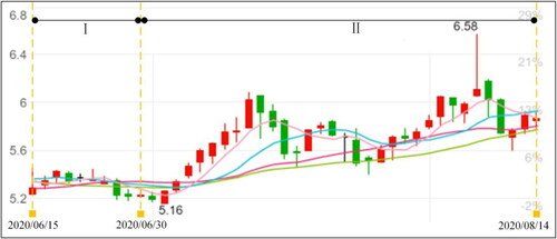
Figure 1 shows the calculation results of Models 1 and 3. Figures 2–5 fully present the share prices of the four stocks including the studied data. From Figures 2–5, we can find that each Part I provides the share price trend of the four stocks from June 15^th to June 30^th and each Part II illustrates the share price trend of the four stocks from July 1^st to August 14^th. Based on these figures, further comparisons are derived as below:

Figure 1. The comparison of optimal investment ratios of investors in Example 3. Source: public data of China’s stock markets (www.wind.com.cn)

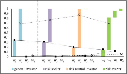
Figure 2. The share prices of GJP. Source: public data of China’s stock markets (www.wind.com.cn)

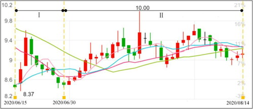
Figure 3. The share prices of ZHG. source: public data of China’s stock markets (www.wind.com.cn)

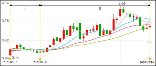
Figure 4. The share prices of JOC. Source: public data of China’s stock markets (www.wind.com.cn)

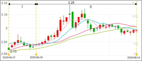
Figure 5. The share prices of QJB. Source: public data of China’s stock markets (www.wind.com.cn)

1. Figure 1 clarifies that the optimal investment ratios for general investors and the three types of risk investors based on the Model 1 are different.

2. According to Figure 1, it is reasonable for general investors to invest more money in ZHG $x_2$ and put the remaining investment in GJP $x_1.$ In this way, general investors can obtain the maximum returns. Meanwhile, the share prices of ZHG $x_2$ and GJP $x_1$ from June 15^th to June 30^th further prove this conclusion. Therefore, it is suitable for general investors to select these two stocks to obtain the maximum return.

3. Compared with the three types of risk investors in Figure 1, a risk seeker invests all of the money on GJP $x_1$ and ZHG $x_2.$ A risk-neutral investor puts the most funds in ZHG $x_2$ and diversifies other funds into GJP $x_1$ and JOC $x_3.$ A risk averter gives more than half of the money to ZHG $x_2$ and puts the rest to the GJP $x_1,$ JOC $x_3,$ and QJB $x_4.$ From Part I of Figures 2–5, we can find that the returns of GJP $x_1$ and ZHG $x_2$ are larger than those of JOC $x_3$ and QJB $x_4,$ indicating that they have greater risks and higher returns. Therefore, GJP $x_1$ and ZHG $x_2$ would be preferred by risk seekers. For a risk averter, Part I of Figure 3 shows an upward trend in the early and later stages. Therefore, the risk of ZHG $x_2$ is small and it could be the priority for risk averters. Additionally, a risk averter invests remaining funds in GJP $x_1,$ JOC $x_3,$ and QJB $x_4$ at different investment ratios. Obviously, these conclusions are consistent with investors’ risk appetites.

4. Each Part II of Figures 2–5 demonstrates the feasibility of the models proposed so that investors’ decisions can be made based on the optimal investment ratios. The explanations are given as follows: for a general investor, the share prices of GJP $x_1$ and ZHG $x_2$ are on the rise, which can bring greater returns. It is wise to invest all the money in stock GJP $x_1$ and ZHG $x_2$ in the early stage. For a risk seeker, although the share prices of GJP $x_1$ and ZHG $x_2$ fluctuate, the overall trends are still rising. They have greater risks and higher returns which is consistent with the investor’s risk appetite. For a risk averter, the share prices of GJP $x_1,$ ZHG $x_2,$ JOC $x_3,$ and QJB $x_4$ have different upward trends. Therefore, it is reasonable to invest different ratios of money in the four stocks. Therefore, the investor can diversify risks, which is also in line with their investment appetites.

The calculation results of the PHPS and RPHPS models in Models 1 and 3 are further analyzed and presented by Figures 1–5, which proves that the conclusions and models are reasonable.

6. Conclusions

In practical investment decision makings, investors generally pay attention to three aspects of financial products, namely mean, variance and return. However, the return frequency is significant but they are not taken into account. To address this issue, this paper has developed the transformation algorithm and defined PHFD. PHFD can consider returns and their occurrence probabilities simultaneously. Besides, to model PHFD and calculate the optimal investment ratios, we have proposed the PHPS and RPHPS models. Based on the maximum-score function or the minimum-deviation function, two PHPS models have been developed to help general investors get the optimal investment ratios. Furthermore, we have proposed the RPHPS models to obtain the optimal investment ratios for the three types of risk investors. Finally, we have provided an empirical study that focuses on four real stocks in China’s stock markets. Under this real background, the feasibility of the proposed models in investment decision makings has been verified.

There are three main contributions in this paper in terms of economics and finance theoretical development as well as practical implications: (1) This paper has developed the transformation algorithm and defined the PHFD, which can simultaneously present the returns of financial products and their occurrence probabilities. (2) This paper has further proposed the PHPS and RPHPS models based on PHFD to obtain the optimal investment ratios for general investors and investors with different risk appetites respectively. (3) This paper has applied the proposed models to an empirical study and proved the models’ feasibility and effectiveness in practical applications.

However, it should be pointed out that there are still some limitations in the proposed portfolio selection models and their application process. For example, although the proposed models can make investment decisions more effectively in the PHFD environment, they are possibly ineffective in the big data environment. Therefore, how to improve these new models to deal with the financial big data is our future research direction.

Disclosure statement

No potential conflict of interest was reported by the authors.

Additional information

Funding

This work was supported by the Natural Science Foundation of China under Grants [72071176 and 71561026] and Applied Basic Research Programs of Science and Technology Commission of Yunnan Province under Grant [2018FD064].

References

- Abdelaziz, F. B., Aouni, B., & Fayedh, R. E. (2007). Multi-objective stochastic programming for portfolio selection. European Journal of Operational Research, 177(3), 1811–1823.
- Alexander, G. J., & Baptista, A. M. (2002). Economic implications of using a mean-VaR model for portfolio selection: A comparison with mean-variance analysis. Journal of Economic Dynamics & Control, 26(7–8), 1159–1193.
- Atanassov, K. T. (1986). Intuitionistic fuzzy sets. Fuzzy Sets & Systems, 20(1), 87–96.
- Bermúdez, J. D., Segura, J. V., & Vercher, E. (2012). A multi-objective genetic algorithm for cardinality constrained fuzzy portfolio selection. Fuzzy Sets & Systems, 188(1), 16–26.
- Brandtner, M., Kürsten, W., & Rischau, R. (2018). Entropic risk measures and their comparative statics in portfolio selection: Coherence vs. convexity. European Journal of Operational Research, 264(2), 707–716. https://doi.org/https://doi.org/10.1016/j.ejor.2017.07.007
- Castellacci, G., & Siclari, M. J. (2003). The practice of delta-gamma VaR: Implementing the quadratic portfolio model. European Journal of Operational Research, 150(3), 529–545. https://doi.org/https://doi.org/10.1016/S0377-2217(02)00782-8
- Chen, W., Li, S. S., Zhang, J., & Mehlawat, M. K. (2020). A comprehensive model for fuzzy multi-objective portfolio selection based on DEA cross-efficiency model. Soft Computing, 24(4), 2515–2526. https://doi.org/https://doi.org/10.1007/s00500-018-3595-x
- Chen, G. H., Luo, Z. J., Liao, X. L., Yu, X., & Yang, L. (2011). Mean–variance–skewness fuzzy portfolio selection model based on intuitionistic fuzzy optimization. Procedia Engineering, 15, 2062–2066. https://doi.org/https://doi.org/10.1016/j.proeng.2011.08.385
- Chen, Z. P., Peng, S., & Lisser, A. (2020). A sparse chance constrained portfolio selection model with multiple constraints. Journal of Global Optimization, 77(4), 825–852. https://doi.org/https://doi.org/10.1007/s10898-020-00901-3
- Demiguel, V., & Nogales, F. J. (2009). Portfolio selection with robust estimation. Operations Research, 57(3), 560–577. https://doi.org/https://doi.org/10.1287/opre.1080.0566
- Gupta, P., Mehlawat, M. K., Kumar, A., Yadav, S., & Aggarwal, A. (2020). A credibilistic fuzzy DEA approach for portfolio efficiency evaluation and rebalancing toward benchmark portfolios using positive and negative returns. International Journal of Fuzzy Systems, 22(3), 824–843. https://doi.org/https://doi.org/10.1007/s40815-020-00801-4
- Ha, Y. M., & Zhang, H. (2020). Algorithmic trading for online portfolio selection under limited market liquidity. European Journal of Operational Research, 286(3), 1033–1051. https://doi.org/https://doi.org/10.1016/j.ejor.2020.03.050
- Huang, X. X. (2006). Fuzzy chance-constrained portfolio selection. Applied Mathematics & Computation, 177(2), 500–507.
- Huang, X. X. (2011). Minimax mean-variance models for fuzzy portfolio selection. Soft Computing, 15(2), 251–260.
- Inuiguchi, M., & Tanino, T. (2000). Portfolio selection under independent possibilistic informaiton. Fuzzy Sets & Systems, 115(1), 83–92.
- Kar, M. B., Kar, S., Guo, S. N., Li, X., & Majumder, S. (2019). A new bi-objective fuzzy portfolio selection model and its solution through evolutionary algorithms. Soft Computing, 23(12), 4367–4381. https://doi.org/https://doi.org/10.1007/s00500-018-3094-0
- Karnik, N. N., & Mendel, J. M. (2001). Centroid of a type-2 fuzzy set. Information Sciences, 132(1-4), 195–220. https://doi.org/https://doi.org/10.1016/S0020-0255(01)00069-X
- Kwan, C. C. Y. (1997). Portfolio selection under institutional procedures for short selling: Normative and market-equilibrium considerations. Journal of Banking & Finance, 21(3), 369–391.
- Li, D. F. (2018). TOPSIS-based nonlinear-programming methodology for multiattribute decision making with interval-valued intuitionistic fuzzy sets. IEEE Transactions on Fuzzy Systems, 18(2), 299–311.
- Li, S. X. (1995). An insurance and investment portfolio model using chance constrained programming. Omega, 23(5), 577–585.
- Li, W. M., & Deng, X. (2020). Multi-parameter portfolio selection model with some novel score-deviation under dual hesitant fuzzy environment. International Journal of Fuzzy Systems, 22(4), 1123–1119. https://doi.org/https://doi.org/10.1007/s40815-020-00835-8
- Liu, D. H., & Huang, A. (2020). Consensus reaching process for fuzzy behavioral TOPSIS method with probabilistic linguistic q-rung orthopair fuzzy set based on correlation measure. International Journal of Intelligent Systems, 35(3), 494–528. https://doi.org/https://doi.org/10.1002/int.22215
- Liu, J. H., Jin, X., Wang, T. Y., & Yuan, Y. (2015). Robust multi-period portfolio model based on prospect theory and ALMV-PSO algorithm. Expert Systems with Applications, 42(20), 7252–7262. https://doi.org/https://doi.org/10.1016/j.eswa.2015.04.063
- Li, B., Zhu, Y. G., Sun, Y. F., Aw, G., & Teo, K. L. (2018). Multi-period portfolio selection problem under uncertain environment with bankruptcy constraint. Applied Mathematical Modelling, 56, 539–550. https://doi.org/https://doi.org/10.1016/j.apm.2017.12.016
- Ma, J., Song, Q. S., Xu, J., & Zhang, J. F. (2013). Optimal portfolio selection under concave price impact. Applied Mathematics & Optimization, 67(3), 353–390.
- Markowitz, H. M. (1952). Portfolio selection. The Journal of Finance, 7(1), 77–91.
- Mehralizade, R., Amini, M., Gildeh, B. S., & Ahmadzade, H. (2020). Uncertain random portfolio selection based on risk curve. Soft Computing, 24(17), 13331–13345. https://doi.org/https://doi.org/10.1007/s00500-020-04751-9
- Mendel, J. M., & Wu, H. W. (2007). New results about the centroid of an interval type-2 fuzzy set, including the centroid of a fuzzy granule. Information Sciences, 177(2), 360–377. https://doi.org/https://doi.org/10.1016/j.ins.2006.03.003
- Nguyen, T. T., & Gordon-Brown, L. (2012). Constrained fuzzy hierarchical analysis for portfolio selection under higher moments. IEEE Transactions on Fuzzy Systems, 20(4), 666–682. https://doi.org/https://doi.org/10.1109/TFUZZ.2011.2181520
- Östermark, R. (1996). A fuzzy control model (FCM) for dynamic portfolio management. Fuzzy Sets & Systems, 78(3), 243–254.
- Pai, G. A. V. (2017). Fuzzy decision theory based metaheuristic portfolio optimization and active rebalancing using interval type-2 fuzzy sets. IEEE Transactions on Fuzzy Systems, 25(2), 377–391.
- Pap, E., Bošnjak, Z., & Bošnjak, S. (2000). Application of fuzzy sets with different t-norms in the interpretation of portfolio matrices in strategic management. Fuzzy Sets & Systems, 114(1), 123–131.
- Pástor, Ľ. (2000). Portfolio selection and asset pricing models. The Journal of Finance, 55(1), 179–223.
- Rebiasz, B. (2013). Selection of efficient portfolios-probabilistic and fuzzy approach, comparative study. Computers & Industrial Engineering, 64(4), 1019–1032.
- Sarkar, D. (1996). Concavoconvex fuzzy set. Fuzzy Sets & Systems, 79(2), 267–269.
- Simaan, Y. (1997). Estimation risk in portfolio selection: The mean variance model versus the mean absolute deviation model. Management Science, 43(10), 1437–1446.
- Sun, B. Z., Ma, W. M., & Zhao, H. Y. (2014). Decision-theoretic rough fuzzy set model and application. Information Sciences, 283, 180–196. https://doi.org/https://doi.org/10.1016/j.ins.2014.06.045
- Teresa, L., Vicente, L. C., Paulina, M., José, V. S., & Enriqueta, V. (2004). A downside risk approach for the portfolio selection problem with fuzzy returns. Fuzzy Economic Review, 9 (1), 61–77.
- Torra, V., & Narukawa, Y. (2009). On hesitant fuzzy sets and decision [Paper presentation]. IEEE International Conference on Fuzzy Systems (pp. 1378–1382). Jeju Island, Korea.
- Vercher, E., Bermúdeza, J. D., & Segura, J. V. (2007). Fuzzy portfolio optimization under downside risk measures. Fuzzy Sets & Systems, 158(7), 769–782.
- Vilkkumaa, E., Liesiö, J., Salo, A., & Ilmola-Sheppard, L. (2018). Scenario-based portfolio model for building robust and proactive strategies. European Journal of Operational Research, 266(1), 205–220. https://doi.org/https://doi.org/10.1016/j.ejor.2017.09.012
- Watada, J. (2001). Fuzzy portfolio model for decision making in investment. Studies in Fuzziness & Soft Computing, 73, 141–162.
- Wu, Y. N., Xu, C. B., Ke, Y. M., Chen, K. F., & Sun, X. K. (2018). An intuitionistic fuzzy multi-criteria framework for large-scale rooftop PV project portfolio selection: Case study in Zhejiang. China. Energy, 143, 295–309.
- Xia, M. M., & Xu, Z. S. (2011). Hesitant fuzzy information aggregation in decision making. International Journal of Approximate Reasoning, 52(3), 395–407. https://doi.org/https://doi.org/10.1016/j.ijar.2010.09.002
- Xu, Z. S., & Zhou, W. (2017). Consensus building with a group of decision makers under the hesitant probabilistic fuzzy environment. Fuzzy Optimization and Decision Making, 16(4), 481–616. https://doi.org/https://doi.org/10.1007/s10700-016-9257-5
- Yang, X. B., Lin, T. Y., Yang, J. Y., Li, Y., & Yu, D. J. (2009). Combination of interval-valued fuzzy set and soft set. Computers & Mathematics with Applications, 58(3), 521–527.
- Zadeh, L. A. (1965). Fuzzy sets. Information & Control, 8(3), 338–353.
- Zhou, W., & Xu, Z. S. (2018). Portfolio selection and risk investment under the hesitant fuzzy environment. Knowledge-Based Systems, 144, 21–31. https://doi.org/https://doi.org/10.1016/j.knosys.2017.12.020