Banks’ maturity mismatch, financial stability, and macroeconomic dynamics

Abstract

The average maturity of total bank assets has been rising sharply following the 4-trillion-yuan stimulus package proposed by the Chinese government in 2009. This paper investigates the macroeconomic implications of maturity mismatch problem using the Chinese data over the period 2007Q1–2019Q4. We extend the New-Keynesian DSGE framework from several dimensions: (i) financial frictions between banks and households; (ii) multi-period loan contracts; (iii) dynamic differential reserve requirement as a macroprudential regulation tool. After estimating the model with Chinese data, the simulation results indicate that the sluggish adjustment of financing cost caused by maturity mismatch will attenuate the real sector fluctuation, however, the feedback effects will amplify the responses of the banking sector. Meanwhile, a severe maturity mismatch will dampen the effect of the required reserve rate as a tool to keep financial stability when confronted with productivity shock.

Keywords:

• Banks’ Maturity mismatch
• financial stability
• New-Keynesian model

JEL CLASSIFICATION:

• E43
• E51
• G21

1. Introduction

Maturity conversion is one of the key functions of traditional banks. Transferring funds from agents who are in surplus with short-term demand deposits to agents who are in deficit with long-term financing demands, is still the major responsibility of the banking system, despite the financial innovations through the years. One of the most important implications of the Global Financial Crisis is that the excessive maturity mismatch exposes banks to risks that have the potential to threaten not only their stability but also that of the whole financial system. Consequently, excessive maturity mismatch is undesirable from a financial stability perspective (Hellwig, 2008). Though conceptually of great value, existing literature does not study the inefficiency related to excessive maturity mismatch. However, quantify the economic effects of banks’ maturity mismatch is of great importance to design new policies to enhance financial stability.

The China case makes a notable example since the aggregate level of maturity mismatch in commercial banks’ balance sheet have increased significantly in the last decade. As a representative of the emerging market, the external financing of the real economy in China relies heavily on the banking system, since the direct financing market is underdevelopment. Bank loans accounted for over 81.4% of the total amount of social financing (the total amount of fund that the real sector obtains from the financial system) in 2018. However, the long-term loans exploded drastically in the last decade, at the same time, the shares of current deposit in banks’ liability are increasing, which greatly affects the maturity structure of the banking sector (Tian & Zhu, 2014). The maturity mismatch degree of the banking sector increases sharply,¹ which poses a serious threat to financial stability and sustainable economic security. To safeguard financial stability, the central bank of China has been utilizing the restrictions on banks’ reserves as an active macroprudential policy tool called dynamic management of differentiated reserve requirements since 2010.

Against this background, this paper focuses on the implications of maturity mismatch problem in the banking system in China. We try to answer the following questions: what role does the maturity mismatch act in the propagation of macroeconomic dynamics? What is the impact of the maturity mismatch on the effectiveness of reserve requirement as a macroprudential management tool?

To be specific, we empirically investigate the maturity structure characteristics of the banks’ balance sheet in China, by calculating the liquidity mismatch index (LMI) from 2007Q1–2019Q4. Then we incorporate a banking sector with maturity mismatch in a New-Keynesian framework characterized with financial frictions. To assess the quantitative importance of the instability coming from maturity mismatch and the potential gains from macroprudential regulation, we estimated the model with China data from 2007Q1–2019Q4. The model is buffeted by exogenous stochastic disturbances to total factor productivity, the monetary policy, and bank’s net worth. Then we introduce a feedback reserve requirement rule targeting the fluctuations of the credit market to examine the attenuator effect of the differentiated reserve requirements as a macroprudential policy tool in the presence of a banking sector with imbalanced maturity structure.

The incorporation of maturity mismatch in the banking system changes the dynamic relationship between the macroeconomy and financial sector. On the one hand, faced with the infrequent capital adjustment, these firms may not adjust capital to its optimal level in the future, they will choose to sign a long-term contract with banks. Since part of the loans is fixed, the adjustment of the loan rates become sluggish and the real sector is less vulnerable to the loan rates. On the other hand, with the coordination of agency problem and maturity mismatch, the feedback effect on banks’ net worth accumulation will magnify the fluctuation of the banking system. The agency problem generates an incentive constraint for bank managers, thus resulting in a financial accelerator effect. At the same time, maturity mismatch directly influences the current loan supply ability. When bank net worth accumulates, the agency problem and maturity mismatch problem work together, leading to the excessive volatility of the financial system.

Our simulations suggest that although the reserve requirement might help to attenuate the fluctuations of the macroeconomy and the financial system, when the economy is exposed to monetary policy shocks and financial shocks. However, it will cause excess volatility in interest spread when the economy is exposed to supply shocks, especially there existing severe maturity mismatch in the banking system.

The rest of the paper is proceeded as follows. Section 2 reviews the related literature. Section 3 investigates the empirical facts about the characteristics of the maturity structure of the banking system. Section 4 describes the baseline model while Sect. 5 calibrates and estimates the model with China’s data. Section 6 investigates the dynamics of the simulated model and also examines the effectiveness of the differential reserve requirements as a macroprudential policy tool. Conclusions are made in Sect. 7. The Appendix contains additional details.

2. Literature review

The benefits of maturity mismatch and the vulnerability associated with it have long been recognized by the literature (Diamond & Dybvig, 1983; Allen & Gale, 2009). The Global Financial Crisis in 2007 has been a non-linear case that can emerge from excessive maturity mismatch, with structural funding weaknesses being a key driver of banks’ failures (Federico, 2012; Bologna, 2018). Since then, there has been a vastly growing number of empirical literature investigates the connections between maturity mismatch and the realistic topics, such as financial crisis (Rajan & Bird, 2003), interest rate risk (English et al., 2018), and the macroeconomic fluctuations (Gambacorta & Mistrulli, 2004). Apart from the empirical researches, several literatures have built real business cycle theoretical models with long-term loans and loan defaults. Creel et al. (2015) show that the liquidity shortage of the long-term loans may leads to potential bank-runs. Ferrante (2019) builds a DSGE model with a financial sector that includes long-term loans and nominal rigidity. Even though existing literature has emphasized the social costs and potential bank-run associated with excessive maturity mismatch, researches have ignored the role of maturity mismatch in the propagation of exogenous disturbance.

Since the presence of severe maturity mismatch in the Chinese financial sector is officially recognized, there is a strand of the literature that focuses on the measurement the degree of maturity mismatch in banking system of China, including Net Stable Financing Ratio (Pan, Wang, & Tao, 2017), Core Financing Ratio (Lian & Zhang, 2015), Loan-Deposit Ratio (LDR), Liquidity Coverage Ratio (Zeng & He, 2016), and Liquidity Mismatch Index (Liu et al., 2019). A common conclusion has been made that the maturity mismatch in the Chinese banking system has been more and more significant. Another strand of the literature concentrates on the empirical evidences of its macroeconomic implications. Xiang and Zeng (2019) show that the bank’s capability to provide liquidity is reduced resulting from the maturity mismatch in their balance sheets. Liu and Li (2020) find that more short-term loans amplify the negative effect of tight monetary policy on firm loan-financing and investment. Most of the related work is limited to the scope of the individual bank or the banking system level. The implications of maturity mismatch on the economic dynamics in China remains to be investigated.

This paper explores the important task of quantifying the impact of maturity mismatch on the propagation of macroeconomic fluctuations and the involved instability by incorporating banks’ maturity mismatch into a macro model of financial frictions. Conceptually, the closest paper to ours is Andreasen et al. (2013), who study the role of maturity transformation in banks in a real business cycle model. The specifications of the model mainly refer to Andreasen et al. (2013), and we extend the model into a standard New-Keynesian framework with financial frictions introduced by Gertler and Kiyotaki (2010). However, the simulation results of our model are in stark contrast to Andreasen et al. (2013). The presence of the maturity mismatch on banks’ balance sheets could fuel the instability of financial sectors. The examination of the effects of macroprudential policy is another important deviation to Andreasen et al. (2013).

3. Empirical research on maturity mismatch in Chinese banking system

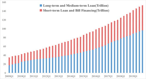
As shown in Figure 1, the proportion of long-term bank loans to the aggregate level was 49.79% in 2009; however, by the end of 2019, it has increased to 62.97%, which may lead to a higher maturity mismatch degree of the banking system. To measure the maturity mismatch problem in the Chinese banking system, we adopt the liquidity mismatch index (LMI) proposed by Brunnermeier et al. (2013).

Figure 1. Maturity structure of Chinese Commercial Banks loan.

Source: Original data is from the People’s Bank of China.

In particular, we take the difference of banks’ weighted assets to weighted liabilities, where assets and liabilities are weighted according to liquidity. The instruments with less liquidity are assigned higher weights. The weights are mainly referred to the prudential regulation practice on maturity transformation adopted by the PBOC adjusted based on the realistic situations of the Chinese banking system. A notable feature of this measure of maturity mismatch is that it is not limited to short-term assets and liabilities, but covers all information of assets and liabilities of the balance sheet, which can measure the liquidity mismatch degree of commercial banks more comprehensively. In addition, the LMI method fully considers the liquidity differences between different assets and liabilities, it is therefore a more accurate proxy of banks’ maturity mismatch than the simpler ratios often used in the literature as we have mentioned before.

Take a representative bank for instance. For asset item $a_t^i$ at time t, it has a weight ${\lambda }_{ai}$ given according to their liquidity. Similarly, liability item $l_t^j$ has a weight ${\lambda }_{bj}.$ Here, ${\lambda }_{ai},{\lambda }_{bj}\in \left[0,1\right]$ . Sum the items of the asset side and liability side in the balance sheet, we get the total liabilityT_l, and total asset T_a. Then we can calculate the liquidity index for the asset side and the liability side (1) $$L_a=\left(\sum {\lambda }_{ai}{a}_t^i\right)/T_a$$(1) (2) $$L_l=\left(\sum {\lambda }_{aj}{b}_t^j\right)/T_l$$(2)

And the liquidity mismatch index can be given as (3) $$LM{I}_t=L_l-L_a$$(3)

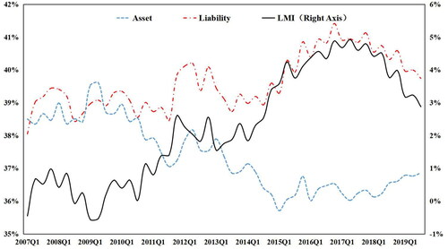
Figure 2 shows the changes of LMI in the banking system of China 2007Q1–2019Q4. Since 2011 the liquidity index of the asset side keeps going down and the liability liquidity index slowly rises, which results in a positive and rising LMI. It is easy to relate these empirical evidences with the credit boom fueled by the 4-trillion stimulus package from late 2008 to 2012. As documented earlier, the credit flows to the entrepreneurs by the long-term contract provided by the banks. This damages the liquidity of the asset side and results in increasing LMI. We take [−2%, 2%] as a security range for LMI following Wang et al. (2013). As shown in Figure 2, since 2012 LMI has always been above the upper bound of the range, and it has an up-going tendency. Though LMI declines due to financial deleveraging after 2017, it maintains a relatively high level. It indicates that the maturity mismatch of China’s banking system is persistent and prominent, which should arouse more attention.

Figure 2. 2007Q1–2019Q4 The changes of LMI in the banking system of China. Note: The original data is from the People’s Bank of China.

4. The model

4.1. Households

We suppose a representative household consumes c_t, provides labor h_t to goods-producing firms and saves d_t for future consumption. The household maximizes the lifetime utility: (4) $$\underset{c_t,M_t,h_t}{\max }{E}_t\sum _{j=0}^{\infty }{\beta }^j\left[\frac{{\left(c_{t+j}-b{c}_{t+j-1}\right)}^{1-{\varphi }_c}}{1-{\varphi }_c}-{\varphi }_2\frac{h_{t+j}^{1+{\varphi }_1}}{1+{\varphi }_1}\right]$$(4) β represents the utility discount factor. ϕ_c represents the coefficient of relative risk aversion and ϕ₁ is the inverse of the elasticity of labor. b denotes the habit intensity for consumption.

Under the following budget constraint, household maintains to maximize their utility: (5) $$c_t+d_t=h_t{w}_t+\frac{R_t^{\mathit{nom}}}{{\pi }_t}{d}_{t-1}+{\Pi }_t$$(5) w_t represents the real wage rates and $R_t^{\mathit{nom}}$ represents the nominal gross interest rate. p_t is the aggregate price level of the final-goods. Here, we define ${\pi }_t=p_t/p_{t-1}$ as inflation. ${\Pi }_t$ is the net transferred wealth from banks to households.

4.2. Firms

4.2.1. Intermediate-goods producing firms

Take a representative intermediate-goods producing firm i for example, the firm produce with a Cobb-Douglas form production function with labor and capital: (6) $$y_{i,t}=a_t{k}_t^{\theta }{h}_{t,t}^{1-\theta }$$(6)

The total productive factor a_t follows AR(1) process: (7) $$\text{ln}\hspace{0.17em}\left({\alpha }_t\right)={\rho }_a\hspace{0.17em}\text{ln}\hspace{0.17em}\left({\alpha }_{t-1}\right)+{\epsilon }_t^{\alpha },{\epsilon }_t^{\alpha }\sim N\left(0,{\sigma }_{\alpha }^2\right)$$(7)

Producing firms hire labor from households and acquire capital with bank loans. The labor can be adjusted in each period but the capital level is not allowed to be adjusted freely. There is a probability ${\alpha }_k$ for firms that are not able to adjust capital to the optimal level ${\tilde{k}}_t$ . The parameter${\alpha }_k$ determines the degree of capital adjustment stickiness. A greater${\alpha }_k$ implies that fewer firms are allowed to adjust the capital level in each period, and the firms will have a longer expectation about the capital adjustment interval. In this circumstance, the adjustment of capital is sticky and we can give the total capital demand of the firms as follows: (8) $$k_t=\left(1-{\alpha }_k\right){\tilde{k}}_t+{\alpha }_k\left(1-\delta \right)k_{t-1}\left(0<{\alpha }_k<1\right)$$(8)

During the interval from time t to time t + j, firms cannot adjust their capital and they maintain to maximize the profits with the optimal capital choice level ${\tilde{k}}_t$ and longer loans maturity at time t. These results in the demand for long-term loan of firms, and one can easily connect the average maturity of the bank loan contracts to the expected capital adjustment interval. $D=1/(1-{\alpha }_k)$ gives the average maturity of long-term contracts.

With the setting of nominal contracts, firms sign the contracts according to the nominal price of the capital stock. Since capital depreciates over time, the firms need to finance ${(1-\delta )}^j{p}_t^k{\tilde{k}}_t$ units of capital. $p_t^k$ represents the nominal price of capital. During the contracts, banks provide fund to the firms at the fixed nominal rental interest rates $r_t^L+\delta$ . To clarify this setup, we let P_t denotes the nominal price level of aggregate output. Consequently, the expression for aggregate firm profit in period t can be given as: (9) $$\mathit{profi}{t}_{t+j|t}=p_{t+j}^{\mathrm{int}}{\left({\left(1-\delta \right)}^j{\tilde{k}}_t\right)}^{\theta }{h}_{t+j|t}^{1-\theta }-w_t{h}_{t+j|t}-\frac{\left(r_t^k+\delta \right)}{{\Pi }_{i=1}^j{\pi }_{t+i}}{\left(1-\delta \right)}^j{\tilde{k}}_t{p}_t^k$$(9) Here, we let $p_t^{\text{int}}$ denotes the real intermediate-goods price. The goods-producing firms determine their capital and labor by maximizing the discount of future profits to present value: (10) $$\underset{{\tilde{k}}_t,h_t}{\max }{E}_t\sum _{j=0}^{+\infty }{\alpha }_k^j{\beta }^j\left[p_{t+j}^{\mathrm{int}}{\alpha }_{t+j}{\left({\left(1-\delta \right)}^j{\tilde{k}}_t\right)}^{\theta }{h}_{t+j|t}^{1-\theta }-w_t{h}_{t+j|t}-\frac{\left(r_t^k+\delta \right)}{{\Pi }_{i=1}^j{\pi }_{t+i}}{\left(1-\delta \right)}^j{\tilde{k}}_t{p}_t^k\right]$$(10)

4.2.2. Capital-goods-producing firms

Introducing capital goods producers is a modeling device to derive market prices for capital (Iacoviello, 2015). Capital producers are competitive firms that obtain the depreciated capital$v_t(1-\delta )$ from intermediate-goods firms and package it with investment i_t and give them back to the intermediate-goods firms. The investment sent to the goods-producing firms results in revenue$v_t^k$ . Capital-producing firm trades capital at the price $p_t^k$ when the contracts are signed. Then we can write the net present value of profits for the capital-goods producing firms as (11) $$\underset{v_t,i_t}{\max }{E}_t\sum _{j=0}^{+\infty }{\beta }^j\frac{{\lambda }_{t+j}}{{\lambda }_t}\left[v_{t+j}-v_{t+j-1}\left(1-\delta \right)-i_{t+j}\right]$$(11) Here, $v_t^k$ denotes the aggregate value of capital, which can be described as (12) $$v_t^k=\left(1-{\alpha }_k\right)\sum _{j=0}^{+\infty }{\alpha }_k^j{p}_{t-j}^k{\left(1-\delta \right)}^j{\tilde{k}}_{t-j}=\left(1-{\alpha }_k\right)p_t^k{\tilde{k}}_t+{\alpha }_k\left(1-\delta \right)v_{t-1}$$(12)

Capital-producing firm faces the constraints described by Eq. (8)(8) $$k_t=\left(1-{\alpha }_k\right){\tilde{k}}_t+{\alpha }_k\left(1-\delta \right)k_{t-1}\left(0<{\alpha }_k<1\right)$$(8) , the devolution of ${\tilde{k}}_t$ , and the accumulation process for the aggregate capital following the work of Christiano et al. (2005) (13) $$k_{t+1}=\left(1-\delta \right)k_t+i_t\left[1-\frac{k}{2}{\left(\frac{i_t}{i_{t-1}}-1\right)}^2\right]$$(13)

4.2.3. Retail firms

A retail firm is augmented into the framework to introduce price stickiness, following Bernanke et al. (1999), which is also a widely accepted way to produce final goods and pricing (Christiano et al., 2005). The final goods output of the economy is the CES function of the distinctive retail goods: (14) $$y_t={\left[{\int }_0^1{y}_{f,t}^{\frac{\eta -1}{\eta }}df\right]}^{\frac{\eta -1}{\eta }}$$(14) Here, $\eta$ represents the demand for elasticity of different retail goods. $y_{f,t}$ represents the production of firm f. The demand function of firm j can be given as (15) $$y_{f,t}={\left(\frac{P_{f,t}}{P_t}\right)}^{-\eta }{y}_t$$(15) $P_{f,t}$ denotes the price of the final-goods of firm j. Then we can give the aggregate level of price: (16) $$P_t={\left[{\int }_0^1{P}_{f,t}^{\eta -1}df\right]}^{\frac{1}{1-\eta }}$$(16)

Following Calvo (1983), we introduce the nominal rigidity into the model. In each period, only $1-{\alpha }_p$ of final-goods firms may adjust their price optimally to level$P_t^{*}$ . The other firms have to keep their price level unchanged. The retail firms choose the optimal price level to maximize their profits: (17) $$\underset{P_t^{*}}{\max }{E}_t\sum _{i=0}^{\infty }{\left({\alpha }_p\beta \right)}^i\frac{{\lambda }_{t+i}}{{\lambda }_t}\left[\frac{P_t^{*}}{P_{t+i}}-p_{t+i}^{\mathrm{int}}\right]y_{f,t+i}$$(17)

4.3. Banks

To connect the model with China’s experiences, we introduce two novel features to the model grounded on China’s economic reality: first, the bank faces a reserve requirement controlled by the central bank. Second, banks’ net worth is supposed to be under the influence of a negative shock. The setting here is based on the fact that the Chinese banking sector identified the upward trend of non-performing loans since 2012, mainly caused by the economic down-turn and industrial transformation, which will continue for many years.

As a representative bank, it uses internal net worth $n_t$ and external short-term deposits from household $d_t$ to provide credit $le{n}_t$ to intermediate-goods producing firms, the balance sheet of the representative bank can be given as followed (18) $$le{n}_t=n_t+d_t$$(18)

Recalling the previous set up that intermediate-goods producing sector is faced with infrequent capital adjustment in each period, this implies the accumulation process of bank revenue$re{v}_t,$ and the total amount of lending$le{n}_t$ can be given as (19) $$\begin{array}{c}le{n}_t=\left(1-{\alpha }_k\right)p_t^k{\tilde{k}}_t+\left(1-{\alpha }_k\right){\alpha }_k\left(1-\delta \right)p_{t-1}^k{\tilde{k}}_{t-1}+\dots \\ =\left(1-{\alpha }_k\right)p_t^k{\tilde{k}}_t+{\alpha }_k\left(1-\delta \right)le{n}_{t-1}{\pi }_t^{-1}\end{array}$$(19) (20) $$re{v}_t=\left(1-{\alpha }_k\right)R_t^k{p}_t^k{\tilde{k}}_t+\left(1-\delta \right){\alpha }_{k}re{v}_{t-1}{\pi }_t^{-1}$$(20) Here,$R_t^{L,\mathit{nom}}$ denotes the nominal gross loan rate. In period t, $(1-{\alpha }_k)$ of the banks’ lending are allocated to the firms that are not able to adjust capital. Similarly, the fraction of fund provided to the firms that adjust their capital stock in period $t-1$ is $(1-{\alpha }_k){\alpha }_k(1-\delta )$ , and so on. As is shown above,${\alpha }_k$ affects the bank’s lending behaviour and correspondingly the credit revenue.

At the beginning of each period, an individual bank manager continues operating with probability$\sigma$ , and exits with probability $1-\sigma$ . The bank managers maintain to maximize the expectation of the discounted continuation value: (21) $$V_t=E_t{\Lambda }_{t,t+1}\left(1-\sigma \right)\left(re{v}_t-r_t^s{d}_t\right)+\sigma E_t{\Lambda }_{t,t+1}{V}_{t+1}$$(21) where${\Lambda }_{t,t+1}$ denotes the discount factor, $\sigma$ represents the surviving ratio of banks.$R_t^s$ denotes the external funding cost of banks. Assume that banks are subjected to reserve requirement $r{r}_t$ controlled by the central bank. Only $(1-r{r}_t)$ of the deposits can be loaned by banks, which can be given by: (22) $$R_t^{L,\mathit{nom}}{d}_t=r_t^s\left(1-r{r}_t\right)d_t+r{r}_t{d}_t$$(22)

The real external funding cost of banks is $r_t^s=\frac{R_t^{nom}-r{r}_t}{1-r{r}_t}.$

Agency Problem: Following Gertler and Kiyotaki (2010), we assume that a costly enforcement problem restraints funding ability of banks from households. The friction in financial intermediation is that bankers can divert a fraction Λ of available funds from the projects they have invested in and transfer them back to their household. If that happens, depositors can force the bank manager into bankruptcy but are assumed to only be able to recover the remaining 1-Λ of assets. Under the agency problem, households will limit the amount of credit issued to the firms. Whenever the value of diverted fund $\Lambda le{n}_t$ is greater than the expected present value of banks $V_t$ , the banker will not stay in the business. The incentive constraint holds with equality if without the constraint the banker has an incentive to divert funds obtained from depositors and go bankrupt instead of continuing to operate with the additional funds: (23) $$V_t\ge \Lambda le{n}_t$$(23)

Once the inventive constraint is binding, the equity capital will limit the banks’ asset. The accumulation of bank net worth$n_t$ is the aggregation of the existing banks and the new-established banks. The transferred fund for the new-established bankers account for the $\epsilon /(1-\sigma )$ fraction of the retired banks net worth $(1-\sigma )n_t$ . Considering the rising importance of financial stability, we introduce an exogenous shock to the bank net worth. It is assumed that banks expose to a net worth shock following Mimir and Sunel (2019). The accumulation process of the net worth for the banking sector can be given by: (24) $$n_{t+1}={\omega }_{t+1}{\pi }_{t+1}^{-1}\left[\sigma \left(re{v}_t-R_t^{s}le{n}_t+R_t^s{n}_t\right)+\epsilon n_t\right]$$(24) ${\omega }_t$ represents the recovery rate of bank net worth after an exogenous shock. The financial shock characterizes the effect of loan losses on the accumulation of banks that may deteriorate the stability of the banking system. The exogenous net worth shock follows an AR(1) process: (25) $$\text{log}\hspace{0.17em}\left({\omega }_t\right)={\rho }_{\omega }\hspace{0.17em}\text{log}\hspace{0.17em}\left({\omega }_{t-1}\right)+{\epsilon }_t^{\omega },{\epsilon }_t^{\omega }\sim N\left(0,{\sigma }_{\omega }^s\right)$$(25)

Alternative Interpretation of the Agency Problem: The agency problem is motivated as bankers’ ability to divert funds for their own use. It creates an incentive compatibility constraint for banks, as depositors would be unwilling to deposit funds were this constraint not to be satisfied. As Iacoviello (2015), we can alternatively motivate the constraint as arising from standard limited commitment problems or by regulatory concerns. For example, the banks’ capital to asset ratio must not be less than a predetermined level, according to the Basel Committee on Banking Supervision.

4.4. Central bank

The nominal interest rates and the reserve requirements are controlled by the central bank to stabilize the output gap and inflation gap: (26) $$\text{ln}\hspace{0.17em}\left(\frac{r_t^{\mathit{nom}}}{r_{ss}^{\mathit{nom}}}\right)={\rho }_r\hspace{0.17em}\text{ln}\hspace{0.17em}\left(\frac{r_{t-1}^{\mathit{nom}}}{r_{ss}^{\mathit{nom}}}\right)+\left(1-{\rho }_r\right)\left({\phi }_{\pi }\hspace{0.17em}\text{ln}\hspace{0.17em}\left(\frac{{\pi }_t}{{\pi }_{ss}}\right)+{\phi }_y\hspace{0.17em}\text{ln}\hspace{0.17em}\left(\frac{y_t}{y_{ss}}\right)\right)+{\epsilon }_t^r$$(26) where$R_t^{\mathit{nom}}\equiv 1+r_t^{\mathit{nom}}$ is the gross interest rate. $r_{ss},{\pi }_{ss},y_{ss}$ are the steady-state values of the nominal interest rate, inflation and output. ${\phi }_{\pi }$ and ${\phi }_y$ are the responding coefficients of the monetary policy to inflation and output, respectively. ${\epsilon }_t^r\sim (0,{\sigma }_r^2)$ denotes an exogenous shock.

4.5. Resource constraint and market clearing

In the equilibrium of the capital market, the aggregate capital of firms equals: (27) $$k_t={\int }_0^1{k}_{i,t}{d}_i$$(27)

In the labor market clears when: (28) $$h_t={\int }_0^1{h}_{i,t}{d}_i$$(28)

The goods market equilibrium necessitates: (29) $$y_t=c_t+i_t$$(29)

5. Calibration and estimation

Following the literature, we estimate the stochastic process parameters using the Bayesian method. The structure parameters are calibrated to the literature and the Chinese economy. According to Chen et al. (2018), the discount factor β is placed at 0.99. The habit intensity parameter b is set to 0.65, consistent with Christiano et al. (2005). The risk aversionϕ_c and the inverse Frisch elasticity ${\varphi }_1$ are both set to 1 following to Yang et al. (2019). In the production sector $\theta$ represents the capital share, which is set at 0.33 according to Andreasen et al. (2013). The depreciation factor is set at 0.025, indicating a 10% annually depreciating rate. The parameter ${\alpha }_p$ that characterize the price stickiness is set to be 0.75, to reflect the fact that the retail firms adjust price every year. The substitution elasticity between intermediate-goods $\eta$ is set to be 6, implying a markup of 20%. The capital parameter featuring the adjustment cost k is set to be 2.5 following Christiano et al. (2005). We fix the required reserve ratio to its steady-state value in the benchmark model (BM), the countercyclical macroprudential policy is also excluded in the Bayesian estimation. Detailed information about the parameter calibration can be found in Table 1.

The parameters governing the banking sector are mostly calibrated based on the study in Yang and Yi (2020). The diverting fraction Λ of banks funding is calibrated to be 0.2. We also calibrate the survive ratio for banks $\sigma$ to 0.972, the newly transferred fund fraction for new banks $\epsilon$ to 0.002.

The parameters characterizing the stochastic process in the model are estimated with Bayesian method. Our data spans a sample of Chinese quarterly series from 2007Q1–2019Q4. All data are extracted from the Wind Financial Database. To diminish the seasonal component and heteroskedasticity, all data are processed with seasonal adjustment and log-linearisation. Then we obtain the cycle component using HP-filter and apply them to the Bayesian estimation. Since we introduce three exogenous shocks in the baseline model, we introduce three economic series for the estimation process: output, inflation rate, and banks’ credit amount. The inflation variable${\pi }_i$ is substituted by the processed fixed base CPI (2007Q1 = 100). Based on that, we obtain the real output$y_t$ by diving the nominal series (GDP) by the inflation rate. The bank credit amount$(le{n}_t)$ is obtained from the total amount of bank loans in the same manner.

We estimate the posterior distribution of the parameters related to the exogenous shocks with Bayesian Markov Chain Monte Carlo methods.² Table 2 represents the prior distribution and posterior distribution of the Bayesian estimation. The prior distributions are mainly referred to literature in China.³ Here, we pay more attention to the parameter characterizing monetary policy. So as to meet with the Blanchard-Kahn conditions, the value of the monetary policy parameters is borrowed from Andreasen et al. (2013). The smoothing parameter${\rho }_r$ follows a Beta-Distribution, the mean of which is set at 0.84 and standard error is set at 0.1. We set the inflation gap coefficient ${\phi }_{\pi }$ priors to 2.37 and the output gap coefficient ${\phi }_y$ to 0.02. The standard deviations are all set to 0.05. The posterior distribution of the parameters is close but significantly different to the prior, which means the estimation result is reasonable and feasible for simulation.

Table 1. Benchmark calibration.

Parameter	Implication	Value	Source
β	Household discount factor	0.99	Chen et al. (2018)
b	Habit formation parameter	0.65	Christiano et al. (2005)
${\varphi }_c$	Household risk aversion	1	Yang et al. (2019)
${\varphi }_1$	Inverse Frisch Elasticity	1	Yang et al. (2019)
θ	Capital share	0.33	Andreasen et al. (2013)
δ	Depreciation rate	0.025	Chen et al. (2018)
${\alpha }_p$	Calvo price adjustment	0.75	Gertler and Kiyotaki (2010)
η	Substitution elasticity	6	Chen et al. (2018)
k	Capital adjustment parameter	2.5	Christiano et al. (2005)
Λ	Fraction of transferred asset	0.20	Yang and Yi (2020)
σ	Bank survival rate	0.972	Yang and Yi (2020)
ε	Start-up fund for new banks	0.002	Yang and Yi (2020)

Source: the parameter estimation results are obtained using Dynare 4.5.7.

Table 2. Prior and posterior distributions of the parameters.

Parameters	Prior			Posterior
	Distribution	Mean	SD	Mean	90% C.I.
${\phi }_{\pi }$	Normal	2.37	0.5	2.8186	2.0699	3.5083
${\phi }_y$	Normal	0.04	0.01	0.0217	0.0098	0.0329
${\rho }_r$	Beta	0.84	0.1	0.7159	0.6312	0.8057
${\rho }_a$	Beta	0.8	0.2	0.9235	0.8004	0.9891
${\rho }_o$	Beta	0.37	0.1	0.3526	0.1981	0.5105
${\sigma }_a$	Inverse gamma	0.1	Inf	0.0298	0.0244	0.0346
${\sigma }_r$	Inverse gamma	0.1	Inf	0.0249	0.0178	0.0318
${\sigma }_o$	Inverse gamma	0.1	Inf	0.6327	0.4581	0.8076

Source: the parameter estimation results are obtained using Dynare 4.5.7.

In addition, we calculate the Laplace approximation of marginal data density of the models with different degrees of maturity mismatch as shown in Table 3. Theoretical model with higher marginal data density captures the characteristics of the reality better. The result shows that the model with a higher mismatch degree has a higher log data density, which means the model can characterize the Chinese economy better. By the way, the data from reality accords with the model with a higher maturity mismatch.

Table 3. Marginal data density.

1	2	3	4	5	6	7	8	9	10
287.122932	287.267206	287.482702	287.751874	288.067836	288.425303	288.81948	289.245639	289.699231	290.175568
11	12	13	14	15	16	17	18	19	20
290.670561	291.18042	291.700726	292.228631	292.760434	293.293536	293.824948	294.352024	294.872138	295.383377

Note: The log data densities are obtained from the Bayesian estimation of models with different values of D.

6. Analyzing the dynamics

6.1. General evaluation of the model

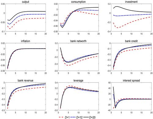
To fully investigate the implications of maturity mismatch in the propagation of macroeconomy and financial system, we assign the average loan maturity D to different values, indicating different levels of maturity mismatch. In the first case, the red dotted lines represent a standard New-Keynesian model with financial frictions but without maturity mismatch, i.e., D = 1. The second cases come close to the average maturity in China and are represented by the bold black lines, i.e., D = 20. The blue-spotted lines indicate the dynamics of a model with a medium degree of maturity mismatch, the average maturity is 3-year, which can be achieved by setting D to 12.

6.1.1. Technological shock

As can be seen, our model, while providing a similar prediction of a “credit attenuator” effect on the fluctuations of real economic activities, suggests that financial fluctuations are magnified. In particular, Figure 3 indicates that, the positive technological shock results in a persistent rise in output and investment, however, the responses of the variables would be more attenuated in the model with maturity mismatch. Under the positive technology shock, households are richer and goods-producing firms are more profitable, both deposits and demands for capital increase. The increasing of capital price boosts the investment of capital-producing firms, which greatly increases their credit demand. In the model without maturity mismatch, the expanding credit demand, which exceeds the expanding credit supply, results in a positive interest spread. These effects work together and generate an increase in banks’ net worth.

Figure 3. Impulse responses to technological shock.

Source: the simulation results are calculated by the authors with Dynare 4.5.7.

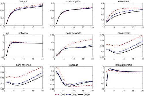
However, with the presence of maturity mismatch, the firm will have a smaller increase in their credit demand compared to the baseline model. At the same time, the long-term loan contracts fix the interest rates, which make the adjustment of interest rate sluggish. The increment of the banks’ net worth is much more weaker in the model with maturity mismatch, which leads to the rise in banks’ leverage ratio. As the result, the interest spread rise and limit the investment increment compared to the model without maturity mismatch.

To discuss the implications of maturity mismatch for the business cycle and financial stability, we report in Table 4 the relative volatility of the model compared to the baseline case without maturity mismatch. The following observations can be made. First of all, the introduction of a severe maturity mismatch problem reinforces the attenuator effects on investments and output resulting from the model without maturity mismatch in the case of the productivity shock. Secondly, It also implicates that banks are subjected to a more fluctuating interest spread, and the volatility of leverage ratio have been amplified slightly from Table 4.

Table 4. Relative volatility of variables in Baseline model.

		Real variables			Financial variables
		Output	Consumption	Investment	Bank revenue	Net worth	Credit	Leverage	Spread
Technological shock	D = 12	0.9952	0.996	0.9896	1.002	1.0003	1.002	1.2664	7.3302
	D = 20	0.9919	0.9932	0.9833	1.0081	1.0059	1.008	1.3335	14.9216
Monetary policy	D = 12	0.2428	0.4387	0.0518	0.5037	0.4701	0.5391	0.644	0.832
	D = 20	0.1185	0.5391	0.1337	0.518	0.5235	0.5603	0.7827	2.2645
Net worth shock	D = 12	0.4624	0.4603	0.4265	0.9978	1.0002	1.0034	0.9793	8.4387
	D = 20	0.1279	0.1267	0.1106	1.0113	1.0134	1.0211	0.9774	18.036

Notes: 1. The results above are the relative rate of the model with maturity mismatch to the Basic Model without maturity mismatch, calculated in a second-order approximation.

2. Relative volatility higher than 1 indicates the variable has greater volatility compared to the basic model.

Source: the simulation results are calculated by the authors with Dynare 4.5.7.

6.1.2. Tight monetary policy experiment

We now check how maturity mismatch impacts on the transmission mechanism of the monetary policy, which are presented in Figure 4. In the baseline model without maturity mismatch, we obtain the standard financial accelerator effect, which has been presented in Gertler and Kiyotaki (2010), amplifies the monetary policy transmission.

Figure 4. Impulse responses to monetary policy.

Source: the simulation results are calculated by the authors with Dynare 4.5.7.

The capital demand decreases as the tight monetary policy increases the funding cost of firms. The downward pressure on banks’ revenue contracts banks’ net worth and leads to a resulting in the incentive constraint. As a consequence, bank credit declines, as well as the output and investment.

In the case of maturity mismatch, the effect of the monetary policy decreases obviously. Faced with fixed multi-period contracts, shocks to the policy rate impact on the funding cost of the newly-issued loans only. As the result, the higher is the maturity mismatch degree, the lower is the proportion of total debt to which new financial terms apply, and the firms are less sensitive to tightening monetary policy. Investments decrease less than in the case without maturity mismatch, which attenuates the fluctuation of the capital price and mitigates the output decline. In addition, the financial accelerator effect is much weaker in the case of maturity mismatch. This is because the lending rate does not rise identically while the policy rate rise. Under this circumstance, the adjustment of total loan is given according to the loan-term loan contracts, the sluggish adjustment of loan rates boost banks’ financial position. The impacts of a tightening monetary on banks’ balance sheets may be weaker compared to the case without maturity mismatch. This result is consistent with the findings drawn in the empirical researches that the transmission of the monetary policy in China is less effective under fixed-rate multi-period contracts (Liu & Li, 2020). At the same time, the weaker responses of the real economy under the monetary policy have also been confirmed in theoretical researches about maturity mismatch like Bianchi and Bigio (2014).

6.1.3. Bank net worth shock

As we already have stressed, the agency problem and maturity mismatch are not only potentially important stand-alone features of the financial system, but they also can generate powerful interactions. This is well illustrated when the economy is buffeted by the financial shock. Figure 5 presents the impulse responses for a fall on banks’ net worth of one standard deviation for different maturity mismatch. In the case without maturity mismatch, a fall in bank net worth will be exacerbated by the financial accelerator generated by the agency problem, which causes total financing by financial intermediaries to shrink. When the incentive constraint binds, the losses in bank net worth raises interest spread due to banks’ inability to extend financing to the firms, which in turn depresses the price of asset and the net worth of banks further, so that investment and output fall dramatically.

Figure 5. Impulse responses to bank net worth shock.

Source: the simulation results are calculated by the authors with Dynare 4.5.7.

In the case of maturity mismatch, the presence of fixed-rate multi-period contracts generates interesting interactions between the transmission of net worth shocks and the proportion of total debt which banks can adjust. Figure 5 makes clear the role played by the maturity mismatch in driving our results: if the degree of maturity mismatch is relatively high, the aggregate effect of the banks’ net worth fall is smaller. Output and investment fall less, interest spread is lower in the long run than the scenario without maturity mismatch. As explained in Mimir & Sunel (2019), the bank capital channel is the main transmission mechanism of financial shocks, to be specific, financial shocks tighten the bank capital constraint and limit the ability of banks to provide credit, thus transmitting the shocks to the real economy. However, with maturity mismatch, the decrease in loan supply resulting from the reduction in banks’ net worth is weakened, thus mitigating the investment and output decline. At the same time, banks cannot adjust loans effectively, which makes the financial system more volatile as is shown in Table 4.

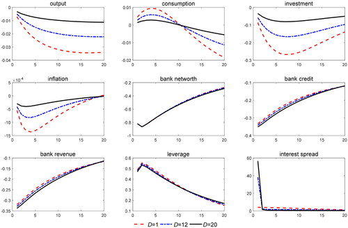
6.2. Macroprudential policy experiment

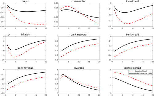
In this part, we undertake a policy experiment to investigate whether a countercyclical policy differentiated reserve requirements can be effective to stabilize the financial sector and the economic activity with maturity mismatch. We compare the different responses to shocks maintaining fixed the reserve requirements with the models in which the differentiated required reserve ratio follows a feedback rule that according to the status of credit supply. Table 5 presents the relative volatility of the policy compared to the baseline model without policy.⁴

Table 5. Relative volatility of variables under macroprudential policy.

		Real variables			Financial variables
		Output	Consumption	Investment	Capital price	Net worth	Credit	Leverage	Spread
Technology shock	D = 1	0.4558	0.5586	0.0906	0.09	0.079	0.0829	0.1644	81.2082
	D = 12	0.455	0.5582	0.0881	0.0893	0.078	0.0823	0.1311	11.42
	D = 20	0.4537	0.5573	0.0858	0.0888	0.0774	0.0818	0.1279	5.8191
Monetary policy	D = 1	0.4668	0.4811	0.3704	0.3955	0.3611	0.3837	0.5839	1.0597
	D = 12	0.7156	0.9671	0.0494	0.5122	0.3226	0.5148	0.5501	0.8954
	D = 20	0.9656	1.0876	1.7466	0.563	0.3308	0.5616	0.5142	0.783
Bank net worth shock	D = 1	0.0938	0.0961	0.1547	0.2883	0.6308	0.2902	0.891	0.3282
	D = 12	0.0077	0.0078	0.013	0.3084	0.6295	0.3105	0.8818	0.5169
	D = 20	0.2456	0.253	0.4106	0.3259	0.6246	0.3279	0.8658	0.5308

Notes: 1. The results above are the relative rate of the model with macroprudential policy to the Baseline Model without policy, calculated in a second-order approximation.

2. A relative volatility higher than 1 indicates the variable has greater volatility compared to the basic model.

Source: the simulation results are calculated by the authors with Dynare 4.5.7.

In the presence of maturity mismatch, given the size and persistence of a shock in monetary policy, it implies smaller volatility for both real and financial variables, than in the counterfactual case without the use of reserve requirement. Moreover, the transmission mechanism of the interest rate is improved. The interest rate increase less than in the counterfactual case and output is controlled better. Under the negative financial shock, the countercyclical policy rule induces a fall in the differentiated required reserve ratio. This makes banks more efficient and less costly to run, which reinforces the internal capital and reduces the potential risks in banks’ net worth. A notable observation is that the macroprudential policy helps to attenuate the amplified impact of the financial shock on bank capital. As the consequence, the rise in credit spreads are lower and bank leverage increases less. To sum up, the macroprudential reserve requirements management that has a first-order impact on the balance sheet of bank with maturity mismatch is the most effective in the event of a financial turmoil.

However, it is not necessarily the case that using a feedback rule for the differentiated required reserve ratio always improves financial stability. Table 5 shows the volatility effects of a productivity shock. A differentiated required reserve ratio on credit moderates macro variables, however, it generates endogenous risk in banking sector. Interest spread becomes more volatile especially with the presence of severe maturity mismatch. It suggests that a countercyclical differentiated required reserve ratio might not be a good stabilizing tool alone in the case of the supply shock. But, it could still be hired as a complementary instrument to monetary policy tools to attenuate the macroeconomic fluctuations.

7. Conclusion

This paper modifies a standard New-Keynesian model with financial friction to consider the typical features of China’s banking sectors– maturity mismatch. Compared to the standard New-Keynesian framework with financial friction, the presence of maturity mismatch alters shocks propagation channel between the macroeconomy and the financial system. On the one hand, diminishing funding costs due to the sluggish adjustment of loan interest rates will mitigate the dynamics of the macroeconomy. On the other hand, the financial accelerator effects will amplify the dynamics of the banking sector with the coordination of agency problem and maturity mismatch. In addition, we also investigate the effectiveness of the differential reserve requirement as a financial stability tool. We find that the countercyclical reserve requirement policy works better than a fixed reserve requirement policy to mitigate the volatility of output when faced with monetary policy and financial shocks.

To fight back the negative effects of the COVID-19 on the economy, the Chinese government has put forward a new set of stimulus plan in 2020. Therefore, the maturity mismatch degree of Chinese banking system may keep on the increasing tendency in the next three to five years. It can be concluded that the policymakers have to focus more on financial stability and take the maturity mismatch problem into consideration. This might be particularly relevant in an economic recovery while the financial sector is still under the stress of government-led deleveraging process.

The imbalance maturity structure of the Chinese banking system might not be a particular case. Actually, under the premise that the economy (especially for the government and the state-owned entrepreneurs) has enormous financing demand, maturity mismatch is the inevitable result of the banking-centered financing system, while bank-centered financing system is the classical characteristic of the developing countries across the world. To some extent, these findings may be useful in developing countries, in which the indirect-financing accounts for the majority of the financing channels of the real economy.

A key hypothesis in this paper is that banks do not hold any other assets other than loans. This leaves no scope for the unconventional monetary policy analysis. However, in China, the traditional monetary policy tool is gradually replaced by unconventional monetary policy, such as lending facilities. To investigate the effects of these unconventional monetary policies, the banking sector in our model needs to be more featured with economic reality, which might be discussed the future research.

Additional information

Funding

This research is supported by the National Natural Science Foundation of China (Grant No.71873055)

Notes

1 After the government’s RBM 4 trillion yuan fiscal stimulus package in 2008, over 60 percents of bank loans are send to infrastructure projects, which require a long horizon and vast funds. Under the New Normal, the Chinese economy is characterized by lower growth speed and the economic structure change. The banks need to provide more long-term loans to satisfy the financing demand, resulting in the rising tendency of maturity mismatch degree of the banking system since 2014.

2 In the Bayesian framework, the prior distributions either reflect subjective opinions or summarize information derived from data sets not included in the estimation sample. And a direct comparison of priors and posterior can provide valuable insights about the extent to which data provide information about the parameters of interest.

3 For parameters between (0,1), the priors are set following the Beta distribution. Parameters higher than zero follow Normal distribution. The exogenous shocks follow an Inverse Gamma distribution.

4 Generally speaking, financial stability is the goal of the prudential authorities. Though some macroprudential policy options being considered may reduce social welfare, one may treat those social losses as the costs of interventions. As the Great Recession in the 1930s reveals, in the absence of any interventions in the pre-crisis period, the social welfare losses are enormous when the crisis materializes.

Appendix 1:

Empirical Research of Maturity Structure of Asset Side in Banking System

After the 4 trillion fiscal stimulus plan, a considerable fraction of bank loans went to the large enterprises and local government financing platform. We investigate the distribution of loans in 16 listed banks, which account for the majority of Chinese banking system. Figure A1 shows loan proportions in total bank loans of the 9 major industries from 2007-2016, these industries occupy over 90% bank loans in total.

Figure 1. Loan Proportions in Total Bank Loans of 9 Major Industries

Note: The original data is collected from Wind Financial Database.

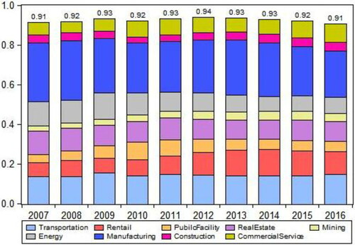
These banks are Bank of Beijing, ICBC Bank (Industrial and Commercial Bank of China), Everbright Bank, Huaxia Bank, CCB Bank (China Construction Bank), BOCOM (Bank of Communication), Minsheng Bank, Bank of Nanjing, Bank of Ningbo, ABC Bank (Agricultural Bank of China), Ping’an Bank, SPD Bank (Shanghai Pudong Development Bank), CIB Bank (Industrial Bank, abbreviated as CIB for historical reasons), CMB Bank (China Merchant Bank), Bank of China, CITIC Bank (Citic Industrial Bank).Then we calculate the loan proportions of 9 major industries in China, including manufacturing, transportation, real estate, energy, mining, construction,public facility, business services, and retail.

The workload in each industry investment project is different, as well as the time needed for complementation. Hence, the average investment horizon differs in industries. The investment horizon is calculated based on the Rate of Construction Projects Completed and Put into Use(RATE). The RATE is the ratio of the number of all complete and put into production projects in a certain period to the number of construction projects in the same period. It is an index reflecting the project construction speed. The investment horizon is taken as the reciprocal of the RATE. The RATE data and the loan data are obtained from National Bureau of Statistics of China. All the results in Table A1 are the average value from 2007-2016. Row 2 and 3 in Table A1 show the average investment horizon of industries and relative horizon of industries to the aggregate level(divide the average horizon of industries by the aggregate horizon). The results show that energy industry, transportation industry, real estate, public facility and commercial services have a longer relative investment horizon larger than 1. And the first three industrial account for over 62.74% of total bank credit. In addition, these industries mostly have monopoly power and implicit government support, they have easier access to bank credit. In conclusion, it can be deduced that asset side of Chinese banking system have a long average maturity.

Table 1. Investment Horizon and Loan Proportions of Industries

Industries	Average Investment Horizon	Relative Investment Horizon	Industrial Loans to Aggregate Domestic Loans
Aggregate	1.57
Mining	1.48	0.9427	2.4757%
Manufacturing	1.53	0.9745	19.9100%
Energy	1.75	1.1146	10.7886%
Construction	1.55	0.9873	0.4014%
Transportation	1.65	1.0510	19.2886%
Retail	1.41	0.8981	1.1143%
Real Estate	1.66	1.0573	32.6643%
Commercial Service	1.72	1.0955	0.9329%
Public Facility	1.72	1.0955	7.9514%

Note: The original data is collected from National Bureau of Statistics of China.

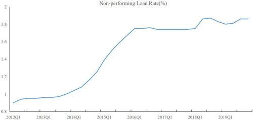
Appendix 2:

Non-performing Loans Rate in China

Due to the increasing downward pressure on the economy and the supply-side structural reform proposed by Chinese Government, the non-performing loan rate in China is increasing rapidly and gradually stabilize since 2012.

Note: The original data is collected from Wind Financial Database.

Appendix 3:

Model Summary

Households: $${\lambda }_t=E_t[{(c_t-b{c}_{t-1})}^{-{\phi }_0}-\beta b{(c_{t+1}-b{c}_t)}^{-{\phi }_0}]$$ $$1=E_t\left[\beta \frac{{\lambda }_{t+1}}{{\lambda }_t}\frac{R_t^{\mathit{nom}}}{{\pi }_{t+1}}\right]$$ $${\phi }_2{h}^{{\phi }_1}={\lambda }_t{w}_t$$

Intermediate-goods producers: $$z_{1,t}=(r_t^{L,\mathit{nom}}+\delta )p_t^k{z}_{2,t}$$ $$z{}_{1,t}=p_t^{\mathrm{int}}\theta a_t{\left(\frac{w_t}{p_t^{\mathrm{int}}{a}_t(1-\theta )}\right)}^{-\frac{1-\theta }{\theta }}+E_t\left[\frac{{\lambda }_{t+1}}{{\lambda }_t}z{}_{1,t+1}(1-\delta ){\alpha }_k\beta \right]$$ $$z_{2,t}=1+E_t[\frac{{\lambda }_{t+1}}{{\lambda }_t}\frac{1}{{\pi }_{t+1}}((1-\delta ){\alpha }_k\beta )z{}_{2,t+1}]$$ $$h_t={\left(\frac{w_t}{p_t^{\mathrm{int}}{a}_t(1-\theta )}\right)}^{-\frac{1}{\theta }}{k}_t$$ $$k_t=(1-{\alpha }_k)\stackrel{\sim }{k_t}+{\alpha }_k(1-\delta )k_{t-1}$$

Retailers: $${\pi }_t={[(1-{\alpha }_p){(\frac{P_t^{*}}{P_t}{\pi }_t)}^{1-\eta }+{\alpha }_p]}^{\frac{1}{1-\eta }}$$ $$nu{m}_t=\frac{\eta }{\eta -1}{p}_t^{\mathrm{int}}{y}_t+E_t\left[{\alpha }_p\beta \frac{{\lambda }_{t+1}}{{\lambda }_t}{\pi }_{t+1}^{\eta -1}nu{m}_{t+1}\right]$$ $$de{n}_t=y_t+E_t\left[{\alpha }_p\beta \frac{{\lambda }_{t+1}}{{\lambda }_t}{\pi }_{t+1}^{\eta -1}de{n}_{t+1}\right]$$ $$\frac{P_t^{*}}{P_t}=\frac{nu{m}_t}{de{n}_t}$$

Banks: $$n{w}_{t+1}=(1-\tau ){\pi }_{t+1}^{-1}(re{v}_t-R_t^{\mathit{nom}}le{n}_t+R_t^{\mathit{nom}}{n}_t)+\epsilon n_t$$ $$n_{t+1}={\omega }_{t}n{w}_{t+1}$$ $$re{v}_t=(1-{\alpha }_k)R_t^{L,\mathit{nom}}{p}_t^k{\stackrel{\sim }{k}}_t+(1-\delta ){\alpha }_{k}re{v}_{t-1}{\pi }_t^{-1}$$ $$le{n}_t=(1-{\alpha }_k)p_t^k{\stackrel{\sim }{k}}_t+(1-\delta ){\alpha }_{k}le{n}_{t-1}{\pi }_t^{-1}$$ $$le{v}_t\equiv \frac{le{n}_t}{n_t}=\frac{x_{2,t}}{\frac{\Lambda }{1-\tau }-x_{1,t}}$$ $$x_{1,t}=E_t(1-{\alpha }_b)\beta \frac{{\lambda }_{t+1}}{{\lambda }_t}{\pi }_{t+1}^{-1}(\frac{re{v}_t}{le{n}_t}-R_t^{\mathit{nom}})+E_t\left({\alpha }_b\beta x_{1,t+1}\frac{le{n}_{t+1}}{le{n}_t}\frac{{\lambda }_{t+1}}{{\lambda }_t}\right)$$ $$x_{2,t}=(1-{\alpha }_b)E_t\left(\beta \frac{{\lambda }_{t+1}}{{\lambda }_t}{\pi }_{t+1}^{-1}\right)R_t^{\mathit{nom}}+E_t\left(x_{2,t+1}{\alpha }_b\beta \frac{n_{t+1}}{n_t}\frac{{\lambda }_{t+1}}{{\lambda }_t}\right)$$

Capital-producers: $$u_{1,t}=\delta +E_t[\beta \frac{{\lambda }_{t+1}}{{\lambda }_t}{\pi }_{t+1}^{-1}{u}_{1,t+1}{\alpha }_k(1-\delta )]$$ $$k_{t+1}=(1-\delta ){\psi }_t{k}_t+i_t[1-\frac{k}{2}{(\frac{i_t}{i_{t-1}}-1)}^2]$$ $$1=q_t(1-\frac{k}{2}{(\frac{i_t}{i_{t-1}}-1)}^2-k(\frac{i_t}{i_{t-1}}-1)\frac{i_t}{i_{t-1}})+E_t\left[\beta \frac{{\lambda }_{t+1}}{{\lambda }_t}{q}_{t+1}k\right(\frac{i_{t+1}}{i_t}-1\left)\frac{i_{t+1}^2}{i_t^2}\right]$$ $$q_t+E_t[{\beta }^2\frac{{\lambda }_{t+2}}{{\lambda }_t}{u}_{1,t+2}{\alpha }_k(1-\delta )p_{t+2}^k]=E_t\left[\beta \frac{{\lambda }_{t+1}}{{\lambda }_t}{u}_{1,t+1}{p}_{t+1}^k\right]+E_t[\beta \frac{{\lambda }_{t+1}}{{\lambda }_t}{q}_{t+1}(1-\delta )]$$

Market clearing: $$y_t=c_t+i_t+m_t$$ $$y_t^{\mathrm{int}}=a_t{k}_t^{\theta }{h}_t^{1-\theta }$$ $$y_t={\Delta }_t^{-1}{y}_t^{\mathrm{int}}$$ $${\Delta }_t=(1-{\alpha }_p){(\frac{P_t^{*}}{P_t})}^{-\eta }+{\alpha }_p{({\pi }_t)}^{\eta }{\Delta }_{t-1}$$

Central bank: $$r{r}_t^{\mathit{nom}}=r{r}_{ss}+{\varphi }_{rr}(\hspace{0.17em}\text{log}\hspace{0.17em}(le{n}_t)-\hspace{0.17em}\text{log}\hspace{0.17em}(le{n}_{t-1}))$$ $$r_t^{\mathit{nom}}=\rho r_{t-1}^{\mathit{nom}}+(1-\rho )(r_{ss}^{\mathit{nom}}+{\phi }_{\pi }\hspace{0.17em}\text{log}\hspace{0.17em}(\frac{{\pi }_t}{{\pi }_{ss}})+{\phi }_y\hspace{0.17em}\text{log}\hspace{0.17em}(\frac{y_t}{y_{ss}}))+{\epsilon }_t^r$$

Shocks: $$ln(a_t)={\rho }_{a}ln(a_{t-1})+{\epsilon }_t^a$$ $$ln({\omega }_t)={\rho }_{\omega }ln({\omega }_{t-1})+{\epsilon }_t^{\omega }$$

Appendix 4:

The stabilizing effects of macroprudential policy

 

Figure 1. Macroprudential Policy experiment with Technological Shock.

Notes: the simulation results are calculated by the authors using Dynare 4.5.7.

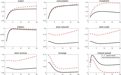
Figure 2. Macroprudential Policy experiment with Monetary Policy Shock.

Notes: the simulation results are calculated by the authors using Dynare 4.5.7.

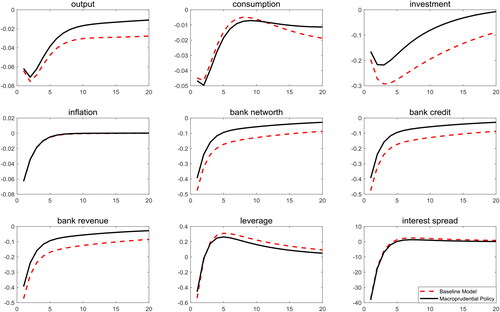
Figure 3. Macroprudential Policy experiment with Bank Net Worth Shock.

Notes: the simulation results are calculated by the authors using Dynare 4.5.7.

References

- Allen, F., & Gale, D. M. (2009). Understanding financial crises. Jahrbücher Für Nationalkonomie Und Statistik, 229(2–3), 343–345.
- Andreasen, M. M., Ferman, M., & Zabczyk, P. (2013). The business cycle implications of banksʼ maturity transformation. Review of Economic Dynamics, 16(4), 581–600. https://doi.org/https://doi.org/10.1016/j.red.2012.12.001
- Bernanke, B. S., Gertler, M., & Gilchrist, S. (1999). The financial accelerator in a quantitative business cycle framework. Handbook of Macroeconomics, 1, 1341–1393.
- Bianchi, J., & Bigio, S. (2014). Banks, Liquidity Management and Monetary Policy, No 20490, NBER Working Papers, National Bureau of Economic Research, Inc.
- Bologna, P. (2018). Banks’ maturity transformation: risk, reward, and policy, No 63, ESRB. IMF Working Papers, 18(45), 1. https://doi.org/https://doi.org/10.5089/9781484345184.001
- Brunnermeier, M., Gorton, G., & Krishnamurthy, A. (2013). Liquidity mismatch measurement. In Risk topography: Systemic risk and macro modeling (pp. 99–112). National Bureau of Economic Research, Inc.
- Chen, Y., Liu, K., & Liu, Z. (2018). U.S. money supply and China's business cycles. Emerging Markets Finance and Trade, 54(5), 957–980. https://doi.org/https://doi.org/10.1080/1540496X.2017.1417833.
- Christiano, L. J., Eichenbaum, M., & Evans, C. L. (2005). Nominal rigidities and the dynamic effects of a shock to monetary policy. Journal of Political Economy, 113(1), 1–45. https://doi.org/https://doi.org/10.1086/426038
- Creel, J., Hubert, P., & Labondance, F. (2015). Financial stability and economic performance. Economic Modelling, 48, 25–40. https://doi.org/https://doi.org/10.1016/j.econmod.2014.10.025
- Diamond, D. W., & Dybvig, P. H. (1983). Bank runs, deposit insurance, and liquidity. Journal of Political Economy, 91(3), 401–419. https://doi.org/https://doi.org/10.1086/261155
- English, W. B., Van den Heuvel, S. J., & Zakrajšek, E. (2018). Interest rate risk and bank equity valuations. Journal of Monetary Economics, 98, 80–97. https://doi.org/https://doi.org/10.1016/j.jmoneco.2018.04.010
- Federico, P. (2012). Developing an index of liquidity-risk exposure: An application to Latin American and Caribbean banking systems. No. 4811, Research Department Publications, Inter-American Development Bank, Research Department.
- Ferrante, F. (2019). Risky lending, bank leverage and unconventional monetary policy. Journal of Monetary Economics, 101, 100–127. https://doi.org/https://doi.org/10.1016/j.jmoneco.2018.07.014
- Gambacorta, L., & Mistrulli, P. E. (2004). Does bank capital affect lending behavior? Journal of Financial Intermediation, 13(4), 436–457. https://doi.org/https://doi.org/10.1016/j.jfi.2004.06.001
- Gertler, M., & Kiyotaki, N. (2010). Financial intermediation and credit policy in business cycle analysis. Handbook of Monetary Economics, 3(3), 547–599.
- Hellwig, M. (2008). The causes of the financial crisis. CESifo Forum, 09(04), 12–21.
- Iacoviello, M. (2015). Financial business cycles. Review of Economic Dynamics, 18(1), 140–163. https://doi.org/https://doi.org/10.1016/j.red.2014.09.003
- Lian, Y., & Zhang, L. (2015). Liquidity shock, bank structure liquidity and credit supply. International Finance Research, 339(4), 64–76.
- Liu, J., Zhao, P., & Tian, J. (2019). Measurement of liquidity risk of commercial Banks based on time-dependent model. Financial Theory and Practice, 40(06), 16–23.
- Liu, H., & Li, M. (2020). Retesting the economic effect of monetary policy on micro enterprises – A Study based on the perspective of loan term structure. Economic Research, 55(02), 117–132.
- Liu, Z. (2013). Research on maturity mismatch risk and governance of joint-stock commercial banks. Ph.D of Huazhong University of Technology.
- Mimir, Y., & Sunel, E. (2019). External shocks, banks, and optimal monetary policy: A recipe for emerging market central banks. International Journal of Central Banking, 15(2), 235–299.
- Pan, M., Wang, Y., & Tao, Y. (2016). Will the regulation of net stable capital ratio affect the risk taking and performance of commercial Banks – Based on empirical evidence of China’s banking industry. Finance and Trade Research, 06, 25–34.
- Rajan, R. S., & Bird, G. (2003). Banks, maturity mismatches and liquidity crises: A simple model. Economia Internazionale, 56(2), 185–192.
- Tian, Y., & Zhu, L. (2014). Influence of mismatching interest rate risks on the maturity of deposits and loans in commercial banks – In the process of interest rate liberalization. Financial Theory and Practice, 421(008), 52–56.
- Wang, Z., Wang, Y., & Chu, X. (2013). Indicator construction and policy tool selection of liquidity management. Shandong Social Sciences, 216(8), 65–69.
- Xiang, H. J., & Zeng, Q. (2019). Maturity mismatch, liquidity Creation and Bank Fragility. Finance and Trade Economics, 040(008), 50–66.
- Yang, L., van Wijnbergen, S., Qi, X., & Yi, Y. (2019). Chinese shadow banking, financial regulation and effectiveness of monetary policy. Pacific-Basin Finance Journal, 57, 101169. https://doi.org/https://doi.org/10.1016/j.pacfin.2019.06.016
- Yang, L., & Yi, Y. (2020). Effectiveness of macroprudential policies under maturity mismatch. Emerging Markets Finance and Trade, 56(12), 2826–2851. https://doi.org/https://doi.org/10.1080/1540496X.2019.1627194
- Zeng, Z., & He, Y. (2016). The influence of liquidity structure of China’s commercial banks on capital cache. International Finance Research, 353(9), 63–74.