The impact of high-frequency economic policy uncertainty on China’s macroeconomy: evidence from mixed-frequency VAR

Abstract

We investigate the impact of high-frequency economic policy uncertainty on investments of state-owned and private-owned enterprises (SOEs and POEs), as well as short-, medium- and long-term bank loans in China by employing the mixed-frequency vector autoregression model. Impulse response analysis suggests that monthly economic policy uncertainty is allowed to have heterogeneous effects on investments and bank loans in China. Variance decomposition analysis shows that aggregating monthly economic policy uncertainty into the quarterly level underestimates the influence of economic policy uncertainty in shaping China’s macroeconomy at business cycle frequencies. By further decomposing the SOEs’ investment, we reveal that the effects of economic policy uncertainty on SOEs’ investment are strengthened due to the existence of the injection of the government investment into SOEs. Trade policy uncertainty has a similar impact on China’s investments and bank loans as economic policy uncertainty. The counterfactual analysis shows that the impact of economic policy uncertainty on China’s investments and bank loans is alleviated when the interest rate channel exists. Our major conclusions are insensitive to a series of robustness checks.

Keywords:

• Economic policy uncertainty
• state-owned enterprises
• bank loans
• trade policy uncertainty
• counterfactual analysis
• mixed-frequency vector autoregression

JEL Classification::

• C32
• E22
• E44

1. Introduction

In the wake of the 2007-2009 global economic crisis (GFC), concerns about the impact of economic policy uncertainty (EPU for short hereafter) have received extensive attention and discussion. In an influential paper, Baker et al. (2016) first quantify the economic policy uncertainty index based on newspaper coverage frequency by employing textual analysis. Subsequently, an increasing number of studies have investigated how economic policy uncertainty affects the macroeconomy and financial markets. Recent studies (Fontaine et al., 2017, 2018) discuss how China’s economic policy uncertainty affects the global economy in view of China’s role as the largest emerging market economy.

In this paper, we depart from previous literature and study how high-frequency economic policy uncertainty affects China’s macroeconomy. Specifically, we investigate the responses of investments (including state-owned and private-owned enterprises)¹ and bank loans (short-, medium- and long-term) at the macro-level. To address this issue, we take advantage of the mixed-frequency vector autoregression (MF-VAR) model developed by Ghysels (2016), which allows us to deal with data of different sampling frequencies and avoids the biased results caused by temporal aggregation of high-frequency economic policy uncertainty. Three key factors make us focus on the responses of investments and bank loans in China to high-frequency economic policy uncertainty.

First, a vast number of papers mainly investigate the micro-level investment data (e.g., listed firms in China) rather than the macro-level investments of state-owned enterprises (SOEs) and private-owned enterprises (POEs). Wang et al. (2014) attempt to answer how economic policy uncertainty influences corporate investment of Chinese listed companies and conclude that firms having a higher return on invested capital will use more internal finance to mitigate the negative effect of policy uncertainty on corporate investment. Wu et al. (2019) study how EPU influences firms’ overseas investments for Chinese listed companies and find a significant negative relationship between EPU and firms’ foreign investments, especially for financially constrained firms and firms relying on government subsidies. Liu and Zhang (2020) design a quasi-natural experiment for the identification of causal relationships between EPU and firms’ investment-financing decisions by collecting nonfinancial firms listed in China’s A-share stock market and show that economic policy uncertainty significantly impedes real investment and reduces net debt issuance for private firms, whereas no such effects exist in state-owned firms. A similar study conducted by Zhang et al. (2015) uncovers that Chinese listed firms tend to lower their leverage ratios as the degree of economic policy uncertainty increases.

Different from the aforementioned research based on the micro-level data, we turn to study how economic policy uncertainty affects the investments of SOEs and POEs at the macro-level. It is worth pointing out that investment at the macro-level eliminates the idiosyncratic behaviors and avoids the biased results generated by employing the samples of only listed companies because macro-level investments of SOEs and POEs incorporate the nonlisted firms and listed companies. More importantly, macro-level empirical findings provide supplementary evidence for the existing theoretical analysis (Chang et al., 2016; Li & Luo, 2019). Therefore, how economic policy uncertainty affects the aggregate investment patterns of SOEs as well as that of POEs will be a pivotal focus in our study.

Historically, no matter in the SOE-led economy (1978-1997) or the investment-driven economy (1998-2015), state-owned enterprises in China dominate and enjoy the preferential credits and credit loans with depressing interest rates for a long time (Chen & Zha, 2018). Therefore, another important issue is how economic policy uncertainty affects China’s financial markets, especially the behaviors of bank loans with different maturities. Recent studies only discuss how China's EPU affects stock markets working as a direct financing channel rather than bank loans acting as a major indirect channel in China. Chen et al. (2017) examine the impact of China’s EPU on the time-series variation of the Chinese stock market expected returns. Furthermore, Li (2017) demonstrates that China’s EPU commands a positive equity premium of China’s stock market. At the end of 2018, bank loans dominate the external financing for China's firms (around 50%) and the stock market only plays a very limited role in the external financing (around 10%). In China, bank loans to nonfinancing firms will provide financing services for important short-run to long-run national economic initiatives. Hence, different maturities of bank loans reflect the preferential and biased lending policy guided by the Chinese government. As Chang et al. (2016) point out, the link between the government’s investment in the heavy sector (usually major SOEs) and its priority in injecting long-term bank loans into this sector is an unusual institutional arrangement in China.

Finally, investments and bank loans in China are usually published at a lower frequency (e.g., annual or quarterly), however, China’s economic policy uncertainty is measured at a higher frequency (e.g., monthly or daily). Therefore, to investigate the impact of economic policy uncertainty on investments and bank loans at the macro-level, we should retrieve a quarterly average of economic policy uncertainty for further analysis. Nevertheless, recent studies (Ferrara & Guérin, 2018; Motegi & Sadahiro, 2018) demonstrate that lowering the frequency of high-frequency uncertainty shock to make all variables have a single frequency in the estimation framework might give rise to potentially mis-specifying the co-movements of macroeconomic variables and misleading the subsequent impulse response analysis. Ferrara and Guérin (2018) document that uncertainty measures are typically available at a high frequency (daily or monthly), and conclude that we shouldn’t omit the mixed-frequency nature of the macroeconomic variables and should further examine the impact of uncertainty shocks on macroeconomy by employing high-frequency data rather than aggregating the high-frequency uncertainty to match the lower frequency of macroeconomic variables. Also, Motegi and Sadahiro (2018) estimate a mixed frequency vector autoregression (MF-VAR) and confirm that an advantage of MF-VAR is that monthly stock prices are allowed to have heterogeneous impacts on the other quarterly series.

In this paper, we take a fresh look at how China’s high-frequency economic policy uncertainty affects the interest rate, macro-level investments of state-owned enterprises and private-owned enterprises as well as bank loans at lower frequency through the empirical framework of the mixed-frequency vector autoregression model (MF-VAR). The MF-VAR model not only helps us understand the economic policy uncertainty affects China’s investments and bank loans at the macro-level but also allows us to identify the heterogeneous effects of high-frequency economic policy uncertainty. We also study how high-frequency trade policy uncertainty affects China’s macroeconomy and financial markets in light of the intensified US-China conflict since 2018.² One similar study by Yan and An (2020) evaluates the effects of high-frequency US uncertainty shocks on China’s investments and bank loans through the mixed-frequency vector autoregression model and concludes that time-stamped US uncertainty shocks generate partly heterogeneous impacts on China’s investments and bank loans. However, our paper will be different from their research in two major aspects. First, we introduce interest rate as a new channel to understand how interest rate interacting with the economic policy uncertainty shapes Chinese macroeconomy and financial markets together. The transmission channel of uncertainty shock through the interest rate is also supported by Choi and Shim (2019). Second, we use economic policy uncertainty in our benchmark model and trade policy uncertainty in our extended research rather than the financial uncertainty proxied by the VIX index used by Yan and An (2020). Pastor and Veronesi (2017) find that there is a puzzle of high policy uncertainty and low financial uncertainty, in particular, a divergence between them implies that high policy uncertainty has not translated into high financial market volatility effectively after 2011.³ Therefore, it is a more interesting issue to explore how high-frequency economic policy uncertainty affects China’s investments and bank loans in light of the characteristics of a policy-driven economy.

A number of salient facts emerge from our analysis using mixed-frequency VAR models. We first investigate the impact of high-frequency China’s economic policy uncertainty on SOEs’ and POE’s investments, as well as short-, medium- and long-term bank loans by employing the mixed-frequency vector autoregression framework. Impulse response analysis suggests that China’s time-stamped economic policy uncertainty generates partly heterogeneous impacts on China’s investments and bank loans, which is likely to be covered by using the traditional quarterly VAR model. Variance decomposition analysis finds that aggregating monthly economic policy uncertainty into a quarterly level underestimates the influence of economic policy uncertainty in shaping China’s macroeconomy.

By further decomposing the SOEs’ investment, we reveal that the effects of economic policy uncertainty on SOEs’ investment are strengthened due to the existence of the injection of the government investment into state-owned enterprises. A counterfactual experiment is also conducted to address the following issue that to what extent economic policy uncertainty through the interest rate transmission channel contributes to aggregate fluctuations in China. The counterfactual analysis shows that the impact of economic policy uncertainty on China’s investments and bank loans are alleviated when the interest rate channel exists. In addition, by introducing trade policy uncertainty in view of intensified US-China trade conflict, we find that trade policy uncertainty will have a similar influence on China’s investments and bank loans as economic policy uncertainty.

There are three main contributions in our paper. First, our paper investigates the impact of China’s economic policy uncertainty on the domestic macroeconomy and financial markets, in particular, we consider two different types of investment (SOEs and POEs) and different maturities of bank loans, whereas seldom previous studies ever empirically explore their responses to EPU shock in a systemic framework. Second, many empirical strategies have been unearthed to examine the effects of economic policy uncertainty, e.g., the global vector autoregressive (GVAR) model employed by Han et al. (2016). However, not many applied papers use MF-VAR so far, since it is a relatively new tool. Therefore, our paper complements the empirical studies by employing a mixed-frequency VAR model to examine the impact of high-frequency variables on low-frequency variables. Third, existing studies only examine the spillover effects of China’s monthly EPU on other economies rather than on domestic macroeconomic and financial conditions, in particular, the effects of uncertainty on the economy could well be non-linear in that, in specific episodes, uncertainty could severely affect economic activity, but instead have little or no effect in other times. For example, Fontaine et al. (2017) study the spillover effects of monthly EPU from China on US real macroeconomic variables in both expansion and recession periods and confirm that China’s EPU significantly affects US economic activity during busts while no effect is perceptible during booms. Furthermore, Fontaine et al. (2018) investigate the spillover effects from a shock to China’s EPU based on monthly EPU data and find important asymmetries in the responses to Chinese uncertainty shocks of macro-variables, especially for the US, the Euro Area, and South Korea during the periods of busts rather than that of booms.⁴

The remainder of this paper is organized as follows. Section 2 presents and discusses the mixed-frequency vector autoregression (MF-VAR) methodology. Section 3 explains the data source and performs preliminary descriptive statistics. Section 4 investigates the main empirical results with the help of impulse responses and variance decompositions. Section 4 conducts a series of robustness checks for the benchmark model. The last section concludes this paper.

2. Empirical strategy

We start with a single-frequency VAR model and then construct a mixed-frequency VAR model to exploit how sampling frequency changes the results substantially and attempt to understand how the single-frequency VAR model biases our empirical results in the subsequent analysis.

2.1. Quarterly VAR: A single-frequency model

We denote quarter t, where $\mathrm{t}\in \{1,2,3,4\}.$ Let EPU be a quarterly economic policy uncertainty (EPU) index. Let be ${\mathrm{R}}_{\mathrm{IB}}$ be the interbank interest rate in China. Let ${\mathrm{I}}_{\mathrm{SOE}}$ be the investment of state-owned enterprises (SOEs). Similarly, let ${\mathrm{I}}_{\mathrm{POE}}$ be the investment of private-owned enterprises (POEs). Furthermore, let ${\mathrm{BL}}_{\mathrm{S}}$ and ${\mathrm{BL}}_{\mathrm{ML}}$ be the bank loans to nonfinancial firms in the short term (S) and the medium- and long-term (ML), respectively. Assume that each series is differenced sufficiently to make all series stationary.⁵ More details on the variable definition and data source will be discussed in Section 3.

We formulate a quarterly VAR(4) model as follows: (1) $$\underset{{\mathbf{X}}_{\mathrm{t}}}{\underbrace{\left[\begin{array}{c}{\mathrm{EPU}}_{\mathrm{t}}\\ {\mathrm{R}}_{\mathrm{IBt}}\\ {\mathrm{BL}}_{\mathrm{St}}\\ {\mathrm{BL}}_{\mathrm{MLt}}\\ {\mathrm{I}}_{\mathrm{SOEt}}\\ {\mathrm{I}}_{\mathrm{POEt}}\end{array}\right]}}=\sum _{\mathrm{k}=1}^4\underset{{\mathbf{A}}_{\mathrm{k}}}{\underbrace{\left[\begin{array}{c}{\mathbf{A}}_{1\mathrm{k}}\\ {\mathbf{A}}_{2\mathrm{k}}\\ {\mathbf{A}}_{3\mathrm{k}}\\ {\mathbf{A}}_{4\mathrm{k}}\\ {\mathbf{A}}_{5\mathrm{k}}\\ {\mathbf{A}}_{6\mathrm{k}}\end{array}\right]}}\underset{{\mathbf{X}}_{\mathrm{t}-\mathrm{k}}}{\underbrace{\left[\begin{array}{c}{\mathrm{EPU}}_{\mathrm{t}-\mathrm{k}}\\ {\mathrm{R}}_{\mathrm{IBt}-\mathrm{k}}\\ {\mathrm{BL}}_{\mathrm{St}-\mathrm{k}}\\ {\mathrm{BL}}_{\mathrm{MLt}-\mathrm{k}}\\ {\mathrm{I}}_{\mathrm{SOEt}-\mathrm{k}}\\ {\mathrm{I}}_{\mathrm{POEt}-\mathrm{k}}\end{array}\right]}}+\underset{{\mathbf{u}}_{\mathrm{t}}}{\underbrace{\left[\begin{array}{c} {\mathrm{u}}_{1\mathrm{t}}\\ {\mathrm{u}}_{2\mathrm{t}}\\ {\mathrm{u}}_{3\mathrm{t}}\\ {\mathrm{u}}_{4\mathrm{t}}\\ {\mathrm{u}}_{5\mathrm{t}}\\ {\mathrm{u}}_{6\mathrm{t}}\end{array}\right]}}$$(1) where ${\mathbf{A}}_{\mathrm{jk}},\mathrm{ }\mathrm{j}\in \{1,2,3,4,5,6\}$ represent the $\text{j th}$ row of coefficient matrix ${\mathbf{A}}_{\mathrm{k}}.$ ${\mathbf{u}}_{\mathrm{t}}$ is the disturbance term. The lag length is set to be 4 quarters in order to capture the potential seasonality in our model, as suggested by Motegi and Sadahiro (2018). A constant term is omitted to guarantee enough degree of freedom.

Mathematically, we can express the equations of SOE, POE, ${\mathrm{BL}}_{\mathrm{S}},$ and ${\mathrm{BL}}_{\mathrm{ML}}$ as follows: $${\mathrm{R}}_{\mathrm{IBt}}={\sum }_{\mathrm{k}=1}^4\left[{\mathrm{a}}_{21,\mathrm{k}}{\mathrm{EPU}}_{\mathrm{t}-\mathrm{k}}+{\mathrm{a}}_{22,\mathrm{k}}{\mathrm{R}}_{\mathrm{IBt}-\mathrm{k}}+{{\mathrm{a}}_{23,\mathrm{k}}\mathrm{B}\mathrm{L}}_{\mathrm{St}-\mathrm{k}}+{{\mathrm{a}}_{24,\mathrm{k}}\mathrm{B}\mathrm{L}}_{\mathrm{MLt}-\mathrm{k}}{+\mathrm{a}}_{25,\mathrm{k}}{\mathrm{I}}_{\mathrm{SOEt}-\mathrm{k}}+{\mathrm{a}}_{26,\mathrm{k}}{\mathrm{I}}_{\mathrm{POEt}-\mathrm{k}}\right]+{\mathrm{u}}_{2\mathrm{t}}$$ $${\mathrm{I}}_{\mathrm{SOEt}}={\sum }_{\mathrm{k}=1}^4\left[{\mathrm{a}}_{31,\mathrm{k}}{\mathrm{EPU}}_{\mathrm{t}-\mathrm{k}}+{\mathrm{a}}_{32,\mathrm{k}}{\mathrm{R}}_{\mathrm{IBt}-\mathrm{k}}+{{\mathrm{a}}_{33,\mathrm{k}}\mathrm{B}\mathrm{L}}_{\mathrm{St}-\mathrm{k}}+{{\mathrm{a}}_{34,\mathrm{k}}\mathrm{B}\mathrm{L}}_{\mathrm{MLt}-\mathrm{k}}{+\mathrm{a}}_{35,\mathrm{k}}{\mathrm{I}}_{\mathrm{SOEt}-\mathrm{k}}+{\mathrm{a}}_{36,\mathrm{k}}{\mathrm{I}}_{\mathrm{POEt}-\mathrm{k}}\right]+{\mathrm{u}}_{3\mathrm{t}}$$ $${\mathrm{I}}_{\mathrm{POEt}}={\sum }_{\mathrm{k}=1}^4\left[{\mathrm{a}}_{41,\mathrm{k}}{\mathrm{EPU}}_{\mathrm{t}-\mathrm{k}}+{\mathrm{a}}_{42,\mathrm{k}}{\mathrm{R}}_{\mathrm{IBt}-\mathrm{k}}+{{\mathrm{a}}_{43,\mathrm{k}}\mathrm{B}\mathrm{L}}_{\mathrm{St}-\mathrm{k}}+{{\mathrm{a}}_{44,\mathrm{k}}\mathrm{B}\mathrm{L}}_{\mathrm{MLt}-\mathrm{k}}{+\mathrm{a}}_{45,\mathrm{k}}{\mathrm{I}}_{\mathrm{SOEt}-\mathrm{k}}+{\mathrm{a}}_{46,\mathrm{k}}{\mathrm{I}}_{\mathrm{POEt}-\mathrm{k}}\right]+{\mathrm{u}}_{4\mathrm{t}}$$ $${\mathrm{BL}}_{\mathrm{St}}={\sum }_{\mathrm{k}=1}^4\left[{\mathrm{a}}_{51,\mathrm{k}}{\mathrm{EPU}}_{\mathrm{t}-\mathrm{k}}+{\mathrm{a}}_{52,\mathrm{k}}{\mathrm{R}}_{\mathrm{IBt}-\mathrm{k}}+{{\mathrm{a}}_{53,\mathrm{k}}\mathrm{B}\mathrm{L}}_{\mathrm{St}-\mathrm{k}}+{{\mathrm{a}}_{54,\mathrm{k}}\mathrm{B}\mathrm{L}}_{\mathrm{MLt}-\mathrm{k}}{+\mathrm{a}}_{55,\mathrm{k}}{\mathrm{I}}_{\mathrm{SOEt}-\mathrm{k}}+{\mathrm{a}}_{56,\mathrm{k}}{\mathrm{I}}_{\mathrm{POEt}-\mathrm{k}}\right]+{\mathrm{u}}_{5\mathrm{t}}$$ $${\mathrm{BL}}_{\mathrm{MLt}}={\sum }_{\mathrm{k}=1}^4\left[{\mathrm{a}}_{61,\mathrm{k}}{\mathrm{EPU}}_{\mathrm{t}-\mathrm{k}}+{\mathrm{a}}_{62,\mathrm{k}}{\mathrm{R}}_{\mathrm{IBt}-\mathrm{k}}+{{\mathrm{a}}_{63,\mathrm{k}}\mathrm{B}\mathrm{L}}_{\mathrm{St}-\mathrm{k}}+{{\mathrm{a}}_{64,\mathrm{k}}\mathrm{B}\mathrm{L}}_{\mathrm{MLt}-\mathrm{k}}{+\mathrm{a}}_{65,\mathrm{k}}{\mathrm{I}}_{\mathrm{SOEt}-\mathrm{k}}+{\mathrm{a}}_{66,\mathrm{k}}{\mathrm{I}}_{\mathrm{POEt}-\mathrm{k}}\right]+{\mathrm{u}}_{6\mathrm{t}}$$

Therefore, in the quarterly VAR(4) model, we impose a strong restriction that monthly economic policy uncertainty in each quarter only has a homogeneous impact of ${\mathrm{a}}_{\mathrm{j}1,\mathrm{ }\mathrm{k}}/3$ on five China’s macroeconomic variables for each fixed k.

2.2. Mixed frequency VAR

We now turn to illustrate a mixed-frequency VAR benchmark model which keeps in line with Ghysels (2016), Motegi and Sadahiro (2018), and Yan and An (2020), which incorporates the monthly EPU index rather than the quarterly EPU index, and quarterly ${\mathrm{R}}_{\mathrm{IB}},$ ${\mathrm{I}}_{\mathrm{SOE}},$ ${\mathrm{I}}_{\mathrm{POE}},$ ${\mathrm{BL}}_{\mathrm{S}},$ and ${\mathrm{BL}}_{\mathrm{ML}}.$⁶ To introduce the monthly EPU index into our extended model, let the ${\mathrm{EPU}}_{\mathrm{it}}$ as the $\text{i th}$ month in each quarter t, where $\mathrm{i}\in \{1,2,3\}.$ For example, ${\mathrm{EPU}}_{1\mathrm{t}}$ implies the first month of the first quarter in 2007, then ${\mathrm{EPU}}_{1\mathrm{t}+1}$ means the first month of the second quarter in 2007, which equals the fourth month in 2007. Hence, the quarterly EPU can be interpreted as:

$\mathrm{EPU}=\frac{1}{3}{\sum }_{\mathrm{i}=1}^3{\mathrm{EPU}}_{\mathrm{it}},$ for each quarter t

Specifically, the MF-VAR(4) benchmark model is constructed as follows: (2) $$\underset{{\mathbf{Y}}_{\mathrm{t}}}{\underbrace{\left[\begin{array}{c} {\mathrm{EPU}}_{1\mathrm{t}}\\ {\mathrm{EPU}}_{2\mathrm{t}}\\ {\mathrm{EPU}}_{3\mathrm{t}}\\ {\mathrm{R}}_{\mathrm{IBt}}\\ {\mathrm{BL}}_{\mathrm{St}}\\ {\mathrm{BL}}_{\mathrm{MLt}}\\ {\mathrm{I}}_{\mathrm{SOEt}}\\ {\mathrm{I}}_{\mathrm{POEt}}\end{array}\right]}}=\sum _{\mathrm{k}=1}^4\underset{{\mathbf{B}}_{\mathrm{k}}}{\underbrace{\left[\begin{array}{c}{\mathbf{B}}_{1\mathrm{k}}\\ {\mathbf{B}}_{2\mathrm{k}}\\ {\mathbf{B}}_{3\mathrm{k}}\\ {\mathbf{B}}_{4\mathrm{k}}\\ {\mathbf{B}}_{5\mathrm{k}}\\ {\mathbf{B}}_{6\mathrm{k}}\\ {\mathbf{B}}_{7\mathrm{k}}\\ {\mathbf{B}}_{8\mathrm{k}}\end{array}\right]}}\underset{{\mathbf{Y}}_{\mathrm{t}-\mathrm{k}}}{\underbrace{\left[\begin{array}{c} {\mathrm{EPU}}_{1\mathrm{t}-\mathrm{k}}\\ {\mathrm{EPU}}_{2\mathrm{t}-\mathrm{k}}\\ {\mathrm{EPU}}_{3\mathrm{t}-\mathrm{k}}\\ {\mathrm{R}}_{\mathrm{IBt}-\mathrm{k}}\\ {\mathrm{BL}}_{\mathrm{St}-\mathrm{k}}\\ {\mathrm{BL}}_{\mathrm{MLt}-\mathrm{k}}\\ {\mathrm{I}}_{\mathrm{SOEt}-\mathrm{k}}\\ {\mathrm{I}}_{\mathrm{POEt}-\mathrm{k}}\end{array}\right]}}+\underset{{\mathbf{\epsilon }}_{\mathrm{t}}}{\underbrace{\left[\begin{array}{c} {\mathrm{\epsilon }}_{1\mathrm{t}}\\ {\mathrm{\epsilon }}_{2\mathrm{t}}\\ {\mathrm{\epsilon }}_{3\mathrm{t}}\\ {\mathrm{\epsilon }}_{4\mathrm{t}}\\ {\mathrm{\epsilon }}_{5\mathrm{t}}\\ {\mathrm{\epsilon }}_{6\mathrm{t}}\\ {\mathrm{\epsilon }}_{7\mathrm{t}}\\ {\mathrm{\epsilon }}_{8\mathrm{t}}\end{array}\right]}}$$(2) where ${\mathbf{B}}_{\mathrm{jk}},\mathrm{ }\mathrm{j}\in \{1,2,3,4,5,6,7,8\}$ represents the $\text{j th}$ row of coefficient matrix ${\mathbf{B}}_{\mathrm{k}}.$ ${\mathbf{\epsilon }}_{\mathrm{t}}$ is the disturbance term. The lag length is also set to be 4 for a comparison with the quarterly VAR(4) model in equation (1)(1) $$\underset{{\mathbf{X}}_{\mathrm{t}}}{\underbrace{\left[\begin{array}{c}{\mathrm{EPU}}_{\mathrm{t}}\\ {\mathrm{R}}_{\mathrm{IBt}}\\ {\mathrm{BL}}_{\mathrm{St}}\\ {\mathrm{BL}}_{\mathrm{MLt}}\\ {\mathrm{I}}_{\mathrm{SOEt}}\\ {\mathrm{I}}_{\mathrm{POEt}}\end{array}\right]}}=\sum _{\mathrm{k}=1}^4\underset{{\mathbf{A}}_{\mathrm{k}}}{\underbrace{\left[\begin{array}{c}{\mathbf{A}}_{1\mathrm{k}}\\ {\mathbf{A}}_{2\mathrm{k}}\\ {\mathbf{A}}_{3\mathrm{k}}\\ {\mathbf{A}}_{4\mathrm{k}}\\ {\mathbf{A}}_{5\mathrm{k}}\\ {\mathbf{A}}_{6\mathrm{k}}\end{array}\right]}}\underset{{\mathbf{X}}_{\mathrm{t}-\mathrm{k}}}{\underbrace{\left[\begin{array}{c}{\mathrm{EPU}}_{\mathrm{t}-\mathrm{k}}\\ {\mathrm{R}}_{\mathrm{IBt}-\mathrm{k}}\\ {\mathrm{BL}}_{\mathrm{St}-\mathrm{k}}\\ {\mathrm{BL}}_{\mathrm{MLt}-\mathrm{k}}\\ {\mathrm{I}}_{\mathrm{SOEt}-\mathrm{k}}\\ {\mathrm{I}}_{\mathrm{POEt}-\mathrm{k}}\end{array}\right]}}+\underset{{\mathbf{u}}_{\mathrm{t}}}{\underbrace{\left[\begin{array}{c} {\mathrm{u}}_{1\mathrm{t}}\\ {\mathrm{u}}_{2\mathrm{t}}\\ {\mathrm{u}}_{3\mathrm{t}}\\ {\mathrm{u}}_{4\mathrm{t}}\\ {\mathrm{u}}_{5\mathrm{t}}\\ {\mathrm{u}}_{6\mathrm{t}}\end{array}\right]}}$$(1) . Mathematically, we can express the equations of ${\mathrm{I}}_{\mathrm{SOE}},$ ${\mathrm{I}}_{\mathrm{POE}},$ ${\mathrm{BL}}_{\mathrm{S}},$ and ${\mathrm{BL}}_{\mathrm{ML}}$ as follows: $${\mathrm{R}}_{\mathrm{IBt}}={\sum }_{\mathrm{k}=1}^4\left[\sum _{\mathrm{j}=1}^3{\mathrm{b}}_{4\mathrm{j},\mathrm{k}}{\mathrm{EPU}}_{\mathrm{jt}-\mathrm{k}}+{\mathrm{b}}_{44,\mathrm{k}}{\mathrm{R}}_{\mathrm{IBt}-\mathrm{k}}+{{\mathrm{b}}_{45,\mathrm{k}}\mathrm{B}\mathrm{L}}_{\mathrm{St}-\mathrm{k}}+{{\mathrm{b}}_{46,\mathrm{k}}\mathrm{B}\mathrm{L}}_{\mathrm{MLt}-\mathrm{k}}+{\mathrm{b}}_{47,\mathrm{k}}{\mathrm{I}}_{\mathrm{SOEt}-\mathrm{k}}+{\mathrm{b}}_{48,\mathrm{k}}{\mathrm{I}}_{\mathrm{POEt}-\mathrm{k}}\right]+{\mathrm{\epsilon }}_{4\mathrm{t}}$$ $${\mathrm{I}}_{\mathrm{SOEt}}={\sum }_{\mathrm{k}=1}^4\left[\sum _{\mathrm{j}=1}^3{\mathrm{b}}_{5\mathrm{j},\mathrm{k}}{\mathrm{EPU}}_{\mathrm{jt}-\mathrm{k}}+{\mathrm{b}}_{54,\mathrm{k}}{\mathrm{R}}_{\mathrm{IBt}-\mathrm{k}}+{{\mathrm{b}}_{55,\mathrm{k}}\mathrm{B}\mathrm{L}}_{\mathrm{St}-\mathrm{k}}+{{\mathrm{b}}_{56,\mathrm{k}}\mathrm{B}\mathrm{L}}_{\mathrm{MLt}-\mathrm{k}}+{\mathrm{b}}_{57,\mathrm{k}}{\mathrm{I}}_{\mathrm{SOEt}-\mathrm{k}}+{\mathrm{b}}_{58,\mathrm{k}}{\mathrm{I}}_{\mathrm{POEt}-\mathrm{k}}\right]+{\mathrm{\epsilon }}_{5\mathrm{t}}$$ $${\mathrm{I}}_{\mathrm{POEt}}={\sum }_{\mathrm{k}=1}^4\left[\sum _{\mathrm{j}=1}^3{\mathrm{b}}_{6\mathrm{j},\mathrm{k}}{\mathrm{EPU}}_{\mathrm{jt}-\mathrm{k}}+{\mathrm{b}}_{64,\mathrm{k}}{\mathrm{R}}_{\mathrm{IBt}-\mathrm{k}}+{{\mathrm{b}}_{65,\mathrm{k}}\mathrm{B}\mathrm{L}}_{\mathrm{St}-\mathrm{k}}+{{\mathrm{b}}_{66,\mathrm{k}}\mathrm{B}\mathrm{L}}_{\mathrm{MLt}-\mathrm{k}}+{\mathrm{b}}_{67,\mathrm{k}}{\mathrm{I}}_{\mathrm{SOEt}-\mathrm{k}}+{\mathrm{b}}_{68,\mathrm{k}}{\mathrm{I}}_{\mathrm{POEt}-\mathrm{k}}\right]+{\mathrm{\epsilon }}_{6\mathrm{t}}$$ $${\mathrm{BL}}_{\mathrm{St}}={\sum }_{\mathrm{k}=1}^4\left[\sum _{\mathrm{j}=1}^3{\mathrm{b}}_{7\mathrm{j},\mathrm{k}}{\mathrm{EPU}}_{\mathrm{jt}-\mathrm{k}}+{\mathrm{b}}_{74,\mathrm{k}}{\mathrm{R}}_{\mathrm{IB}-\mathrm{k}}+{{\mathrm{b}}_{75,\mathrm{k}}\mathrm{B}\mathrm{L}}_{\mathrm{St}-\mathrm{k}}+{{\mathrm{b}}_{76,\mathrm{k}}\mathrm{B}\mathrm{L}}_{\mathrm{MLt}-\mathrm{k}}+{\mathrm{b}}_{77,\mathrm{k}}{\mathrm{I}}_{\mathrm{SOEt}-\mathrm{k}}+{\mathrm{b}}_{78,\mathrm{k}}{\mathrm{I}}_{\mathrm{POEt}-\mathrm{k}}\right]+{\mathrm{\epsilon }}_{7\mathrm{t}}$$ $${\mathrm{BL}}_{\mathrm{MLt}}={\sum }_{\mathrm{k}=1}^4\left[\sum _{\mathrm{j}=1}^3{\mathrm{b}}_{8\mathrm{j},\mathrm{k}}{\mathrm{EPU}}_{\mathrm{jt}-\mathrm{k}}+{\mathrm{b}}_{84,\mathrm{k}}{\mathrm{R}}_{\mathrm{IBt}-\mathrm{k}}+{{\mathrm{b}}_{85,\mathrm{k}}\mathrm{B}\mathrm{L}}_{\mathrm{St}-\mathrm{k}}+{{\mathrm{b}}_{86,\mathrm{k}}\mathrm{B}\mathrm{L}}_{\mathrm{MLt}-\mathrm{k}}+{\mathrm{b}}_{87,\mathrm{k}}{\mathrm{I}}_{\mathrm{SOEt}-\mathrm{k}}+{\mathrm{b}}_{88,\mathrm{k}}{\mathrm{I}}_{\mathrm{POEt}-\mathrm{k}}\right]+{\mathrm{\epsilon }}_{8\mathrm{t}}$$ where ${\mathrm{b}}_{\mathrm{ij}}$ represents the $\text{j th}$ element of ${\mathbf{B}}_{\mathrm{ik}}.$ However, because ${\mathrm{b}}_{\mathrm{i}1},$ ${\mathrm{b}}_{\mathrm{i}2},$ and ${\mathrm{b}}_{\mathrm{i}3}$ ($\mathrm{i}\in \{4,5,6,7,8\}$) might have distinct values, therefore, these coefficients allow us to analyze the heterogeneous impacts on the variables we concern about. We further perform impulse response and forecast error variance decomposition for the subsequent analysis. We impose a choice of the Cholesky order and set ${\mathrm{R}}_{\mathrm{IB}}{\to \mathrm{BL}}_{\mathrm{S}}\to {\mathrm{BL}}_{\mathrm{ML}}\to {\mathrm{I}}_{\mathrm{SOE}}\to {\mathrm{I}}_{\mathrm{POE}}$ in our mixed-frequency model. This kind of Cholesky order implies that policy uncertainty as an exogenous driver is independent of China's domestic variables and assumes that the interest rate set by the central bank only contemporaneously reacts to the observed external uncertainty. We also assume that bank loans with different maturities will contemporaneously influence investment as Motegi and Sadahiro (2018).

According to the asymptotic theory, the mixed-frequency VAR model is mathematically equivalent to the classic VAR model, hence, our model specification of equation (2)(2) $$\underset{{\mathbf{Y}}_{\mathrm{t}}}{\underbrace{\left[\begin{array}{c} {\mathrm{EPU}}_{1\mathrm{t}}\\ {\mathrm{EPU}}_{2\mathrm{t}}\\ {\mathrm{EPU}}_{3\mathrm{t}}\\ {\mathrm{R}}_{\mathrm{IBt}}\\ {\mathrm{BL}}_{\mathrm{St}}\\ {\mathrm{BL}}_{\mathrm{MLt}}\\ {\mathrm{I}}_{\mathrm{SOEt}}\\ {\mathrm{I}}_{\mathrm{POEt}}\end{array}\right]}}=\sum _{\mathrm{k}=1}^4\underset{{\mathbf{B}}_{\mathrm{k}}}{\underbrace{\left[\begin{array}{c}{\mathbf{B}}_{1\mathrm{k}}\\ {\mathbf{B}}_{2\mathrm{k}}\\ {\mathbf{B}}_{3\mathrm{k}}\\ {\mathbf{B}}_{4\mathrm{k}}\\ {\mathbf{B}}_{5\mathrm{k}}\\ {\mathbf{B}}_{6\mathrm{k}}\\ {\mathbf{B}}_{7\mathrm{k}}\\ {\mathbf{B}}_{8\mathrm{k}}\end{array}\right]}}\underset{{\mathbf{Y}}_{\mathrm{t}-\mathrm{k}}}{\underbrace{\left[\begin{array}{c} {\mathrm{EPU}}_{1\mathrm{t}-\mathrm{k}}\\ {\mathrm{EPU}}_{2\mathrm{t}-\mathrm{k}}\\ {\mathrm{EPU}}_{3\mathrm{t}-\mathrm{k}}\\ {\mathrm{R}}_{\mathrm{IBt}-\mathrm{k}}\\ {\mathrm{BL}}_{\mathrm{St}-\mathrm{k}}\\ {\mathrm{BL}}_{\mathrm{MLt}-\mathrm{k}}\\ {\mathrm{I}}_{\mathrm{SOEt}-\mathrm{k}}\\ {\mathrm{I}}_{\mathrm{POEt}-\mathrm{k}}\end{array}\right]}}+\underset{{\mathbf{\epsilon }}_{\mathrm{t}}}{\underbrace{\left[\begin{array}{c} {\mathrm{\epsilon }}_{1\mathrm{t}}\\ {\mathrm{\epsilon }}_{2\mathrm{t}}\\ {\mathrm{\epsilon }}_{3\mathrm{t}}\\ {\mathrm{\epsilon }}_{4\mathrm{t}}\\ {\mathrm{\epsilon }}_{5\mathrm{t}}\\ {\mathrm{\epsilon }}_{6\mathrm{t}}\\ {\mathrm{\epsilon }}_{7\mathrm{t}}\\ {\mathrm{\epsilon }}_{8\mathrm{t}}\end{array}\right]}}$$(2) will follow the model specification criteria as a standard VAR model. First, the MF-VAR model should satisfy the regularity condition that all roots of the polynomial ${\det (\mathbf{I}}_8-{\sum }_{\mathrm{k}=1}^4{\mathbf{B}}_{\mathrm{k}}{\mathrm{L}}^{\mathrm{k}})=0$ ($\det$ is the determinant and L is the lag operator) lie outside the unit circle. Second, the error term ${\mathbf{\epsilon }}_{\mathrm{t}}$ should satisfy a covariance stationary process with the finite second moment. The above two assumptions will ensure the consistency of the asymptotic normality of the least-squares estimator of VAR coefficients (${\mathbf{B}}_{\mathrm{ik}}$).

3. Data and preliminary statistics

In this section, we will explain variable selection, data source, and perform preliminary analysis for core variables in this paper.

3.1. Data source

For the measurement of China’s economic policy uncertainty, Baker et al. (2016) define the EPU as the inability to predict the occurrence of economic policy shifts. Refer to Baker et al. (2016), EPU is constructed via newspaper coverage frequency for selected term sets. We have two different China’s EPU indexes. For the first index, Baker, Bloom, and Davis develop China’s EPU based on the South China Morning Post. The index is monthly and runs from January 1995 to the present (we call this BBD-type EPU). For the second index, Davis et al. (2019) develop an index of EPU for China from October 1949 to the present based on mainland newspapers (the Renmin Daily and the Guangming Daily)⁷. We use the BBD-type EPU in our benchmark model but EPU developed by Davis et al. (2019) in the robustness. We also utilize the trade policy uncertainty index constructed by Davis et al. (2019) to investigate the impact of trade policy uncertainty. EPU in China index is collected from www.policyuncertainty.com.

For the interest rate, a unique “dual-track” system continues to feature the Chinese financial system: the benchmark interest rates (deposit and lending rates) published by the People’s Bank of China (PBC) remain the anchor for interest rate pricing of deposits and loans in the banking sector; while the interest rates in money markets and bond markets are fully market-determined. Therefore, we select the 3-month Shanghai Interbank Offered Rate (SHIBOR) as a proxy of the policy rate in our paper. Chong and Liu (2017) compare the effectiveness of Chinese market interest rates, Shanghai Interbank Offered Rate (SHIBOR), and repo rates and conclude that SHIBOR promptly reflects the changes in currency markets which will be an appropriate benchmark interest rate.

For China’s investments and bank loans at the macro-level, we collect four different variables from China’s Macroeconomy: Time Series Data updated by the Federal Reserve Bank of Atlanta. We have state-owned enterprises investment and private-owned enterprises investment. Following Chang et al. (2016), the gross fixed capital formation of state-owned enterprises represents state-owned enterprises’ investment (${\mathrm{I}}_{\mathrm{SOE}}$), similarly, the gross fixed capital formation of private-owned enterprises is state-owned enterprises’ investment (${\mathrm{I}}_{\mathrm{POE}}$). Also, we have end-of-quarter bank loans outstanding to nonfinancial firms in the short-term (${\mathrm{BL}}_{\mathrm{S}}$) as well as in the medium- and long-term (${\mathrm{BL}}_{\mathrm{ML}}$) to reflect the bank loans guided by the specific government policies.

China’s Macroeconomy: Time Series Data is collected from https://www.frbatlanta.org/cqer/research/china-macroeconomy.aspx. We use this dataset rather than the dataset published by Chinese statistical and government agencies because this dataset provides quarterly Chinese macroeconomic and financial data more completely. For the monthly EPU, the sample period spans from 1998M1 to 2017M12. For the quarterly variables, the sample period starts with 1998Q1 and ends with 2017Q12. In the subsequent analysis, we also investigate the impacts of trade policy uncertainty (TPU), the sample period of TPU is from 2000M1 to 2017M12. This sample period mainly reflects the transition of China’s macroeconomy and financial markets after the 1997 Asian Financial Crisis (AFC). In the meanwhile, China’s economy, which is known as the investment-driven economy, is affected by preferential, region-biased and regulatory economic policies.

3.2. Preliminary statistics

Our sample period covers 240 months (80 quarters) from 1998Q1 to 2016Q4. Table 1 reports the sample statistics of all variables in the subsequent analysis. First, the mean, median, minimum, and maximum values of ${\mathrm{EPU}}_1$ and ${\mathrm{EPU}}_3$ are greater than the second month in each quarter (${\mathrm{EPU}}_2$). ${\mathrm{EPU}}_1$ and ${\mathrm{EPU}}_3$ have more similarities compared to ${\mathrm{EPU}}_2.$ Therefore, the heterogeneous features of ${\mathrm{EPU}}_1,$ ${\mathrm{EPU}}_2,$ and ${\mathrm{EPU}}_3$ suggest a potential advantage of employing the MF-VAR model. Second, the average growth rate of SOEs’ investment (2.2%) is smaller than that of POEs’ investment (4.3%), and the average growth rate of short-term bank loans (4.9%) is much larger than that of medium- and long-term bank loans (2.7%). These growth rates reflect the transition of China’s economy during the sample period. Specifically, the SOEs’ investment still dominates but has a smaller growth rate, and the importance of the medium- and long-term bank loans to longer infrastructure construction declines in the subsequent economic stage.

Table 1. Descriptive statistics.

	${\mathrm{EPU}}_1$	${\mathrm{EPU}}_2$	${\mathrm{EPU}}_3$	$\mathrm{EPU}$	${\mathrm{I}}_{\mathrm{SOE}}$	${\mathrm{I}}_{\mathrm{POE}}$	${\mathrm{BL}}_{\mathrm{S}}$	${\mathrm{BL}}_{\mathrm{ML}}$	${\mathrm{R}}_{\mathrm{IB}}$
Mean	146.285	130.905	147.970	141.720	0.022	0.043	0.049	0.027	0.034
Median	116.477	101.360	110.799	104.020	0.018	0.041	0.045	0.026	0.030
Minimum	16.566	9.066	36.857	32.490	−0.059	−0.037	−0.060	−0.023	0.012
Maximum	694.849	475.671	646.911	564.225	0.133	0.167	0.216	0.056	0.086
Std.Dev	111.188	98.931	112.912	99.556	0.035	0.031	0.031	0.015	0.014
Skewness	2.289	1.716	2.056	1.938	0.338	0.936	1.917	−0.252	0.980
Kurtosis	10.617	5.995	7.872	7.153	3.476	6.603	14.691	3.519	4.251
KS (p-value)	1.000*** (0.000)	1.000*** (0.000)	1.000*** (0.000)	1.000*** (0.000)	0.476*** (0.000)	0.485*** (0.000)	0.493*** (0.000)	0.491*** (0.000)	0.505*** (0.000)
AD (p-value)	3.596*** (0.000)	4.076*** (0.000)	5.463*** (0.000)	12.455*** (0.000)	0.408 (0.343)	1.210*** (0.003)	4.807*** (0.000)	0.323 (0.534)	1.522*** (0.000)

Notes: ${\mathrm{EPU}}_1,$ ${\mathrm{EPU}}_2,$ ${\mathrm{EPU}}_3$ represent monthly economic policy uncertainty. $\mathrm{EPU}$ represents quarterly economic policy uncertainty. The sample period covers 240 months (80quarters) from 1998Q to 2017Q4. KS means the results of the Kolmogorov-Smirnov test for normality with the corresponding p-values in the parenthesis. AD means the results of the Anderson-Darling test for normality with the corresponding p-values in the parenthesis.

Source: Authors' calculations.

In Table 1, we also report the Kolmogorov-Smirnov test for normality and the Anderson-Darling test for normality. From the Kolmogorov-Smirnov test, we reject the null hypothesis of normality for all variables at the 1% level. From the Anderson-Darling test, we can’t reject the null hypothesis of normality for SOEs’ investment and medium- and long-term bank loans but we can reject other variables at the 1% level. Therefore, these series don’t have a normal distribution by summarizing two different normality tests. However, as Ghysels (2016) and Motegi and Sadahiro (2018) suggest, the asymptotic theory of MF-VAR models relax the requirement of normal distribution.

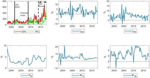
Figure 1 further plots the level trend of EPU and interest rate, and quarter-over-quarter growth rates of 4 variables (${\mathrm{I}}_{\mathrm{SOE}},$ ${\mathrm{I}}_{\mathrm{POE}},$ ${\mathrm{BL}}_{\mathrm{S}},$ and ${\mathrm{BL}}_{\mathrm{ML}}$). The first panel in the first row shows the time trend of economic and trade policy uncertainty in China. It is straightforward to find that joining the WTO and the 2008-2009 GFC gives rise to higher economic policy uncertainty. We also notice that economic policy uncertainty is intensified after 2014 due to China’s New Normal economy and US-China trade war. The second and third panels in the first row show a similar pattern of the growth rate of POEs’ and SOEs’ investment before 2005 but a divergent trend after 2005. The second and third panels in the second-row plot the growth trend of bank loans with different maturities. In particular, the short-term bank loan exhibits larger volatility before 2002 but the growth rates of bank loans with different terms decrease sharply after 2002 because the People’s Bank of China controls credit expansion and implements the safe-loan management for risk prevention.

Figure 1. Time trend for china’s variables.

Notes: EPU and IBR represent economic policy uncertainty (BBD-type, Baker et al., 2016) and 3-Month Interbank Offered Rate, respectively. TPU represents trade policy uncertainty. ${\mathrm{I}}_{\mathrm{SOE}}$ and ${\mathrm{I}}_{\mathrm{POE}}$ represent the investments in state-owned and private-owned enterprises, respectively. ${\mathrm{BL}}_{\mathrm{S}}$ represents bank loans outstanding to nonfinancial firms in the short-term, and ${\mathrm{BL}}_{\mathrm{ML}}$ represents bank loans outstanding to nonfinancial firms in the medium- and long-term. EPU is the monthly level variable and IBR is the quarterly level variable, and the remaining quarterly variables (${\mathrm{I}}_{\mathrm{SOE}},$ ${\mathrm{I}}_{\mathrm{POE}},$ ${\mathrm{BL}}_{\mathrm{S}},$ and ${\mathrm{BL}}_{\mathrm{ML}}$) are quarter-over-quarter growth rates.

Source: Authors' calculations.

4. Empirical results

In this section, we present the empirical results of the impulse response analysis, variance decomposition analysis from different perspectives. First, we report the empirical results for the quarterly and mixed frequency VAR model for benchmark analysis. Second, we investigate how the existence of government investment in state-owned enterprises strengthens the investment behavior of SOEs. Third, we conduct a counterfactual analysis by closing the interest rate transmission channel of economic policy uncertainty to understand the role of interest rate in amplifying or shrinking the impact of economic policy uncertainty shock. Finally, we turn to trade policy uncertainty in light of the intensified US-China trade war since 2018 and address how trade policy uncertainty affects China’s macroeconomy and financial markets.

4.1. Quarterly VAR: A low-frequency analysis

We first discuss the quarterly VAR model. Figure 2 plots the impulse responses of investments and bank loans to one-standard-deviation ($1\mathrm{\sigma }$) EPU shock in the first row and that to interest rate shock in the second row. The dashed lines plot the corresponding 68% bootstrapped confidence intervals.

Figure 2. Impulse responses based on quarterly VAR(4): low-frequency VAR.

Notes: This figure presents the impulse responses of China’s variables to quarterly economic policy uncertainty shock. The solid line plots the impulse response for quarterly horizons (1 to 12). The dashed lines plot the corresponding 68% bootstrapped confidence intervals.

Source: Authors' calculations.

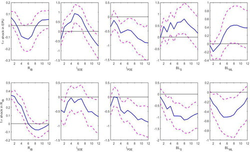
The impulse response function of the interbank interest rate to a $1\mathrm{\sigma }$ EPU shock is positive (0.1%), which is consistent with the findings of Choi and Shim (2019) by using the local projection method under the VAR framework. To mitigate the impact of economic policy uncertainty, the central bank will decrease rather than increase the benchmark rate. However, the quarterly VAR model is unable to characterize the policy process of the PBC and fails to capture the real responses of the PBC.

Next, given the impulse responses of investments of SOEs and POEs to a $1\mathrm{\sigma }$ EPU shock, they both decrease in the first period, while the response of SOEs’ investment is slightly negative compared to that of POEs’ investment. In theory, firms tend to delay their investment in the face of higher uncertainty, which is known as real options (Bernanke, 1983; McDonald & Siegel, 1986; Bloom, 2009, 2014). However, Lin et al. (1998) point out SOEs have dual goals in China for maximizing the profits as private enterprises and achieving specific policy goals of government, and they might increase their investment for pursuing specific policy goals, such as 4-trillion stimulus program during the 2008-2009 global financial crisis. Yan and An (2020) also support the finding that SOEs’ investment tends to increase in an uncertain environment. So, we doubt that the quarterly VAR(4) model makes the results of impulse responses biased.

Furthermore, in view of the bank loans with different maturities, the short-term bank loans tend to have a positive response to economic policy uncertainty shock but medium- and long-term bank loans are more likely to have a negative response to evaluating economic policy uncertainty. It is worth noting that the Chinese government tends to inject massive credits into medium- and long-term investment projects in the form of medium- and long-term bank loans to nonfinancing firms (Chang et al., 2016). In sum, lowering the medium- and long-term banks loan in response to higher economic policy uncertainty can’t accurately capture the behaviors of the Chinese government during the investment-driven periods.

Finally, we turn to discuss the forecast error variance decomposition of quarterly VAR(4) (See Table 2). Intuitively, the forecast error variance decomposition of quarterly VAR(4) only confirms the limited power of economic policy uncertainty in explaining the movements in investments and bank loans. At the prediction horizon of $\mathrm{h}=12,$ EPU only accounts for 2.586%, 1.139%, 1.304%, and 6.307% fluctuations in ${\mathrm{I}}_{\mathrm{SOE}},$ ${\mathrm{I}}_{\mathrm{POE}},$ ${\mathrm{BL}}_{\mathrm{S}},$ and ${\mathrm{BL}}_{\mathrm{ML}},$ respectively. Therefore, to some extent, the quarterly VAR model only plays a weak role in explaining the fluctuations of China’s investments and bank loans caused by economic policy uncertainty.

Table 2. Forecast error variance decomposition of quarterly VAR(4).

Decomposition	Shocks	Horizons
		$\mathrm{h}=4$	$\mathrm{h}=8$	$\mathrm{h}=12$
${\mathrm{R}}_{\mathrm{IB}}$	$\mathrm{EPU}$	9.374	24.203	20.835
	${\mathrm{R}}_{\mathrm{IB}}$	75.532	55.834	51.731
Decomposition	Shocks	Horizons
		$\mathrm{h}=4$	$\mathrm{h}=8$	$\mathrm{h}=12$
${\mathrm{BL}}_{\mathrm{S}}$	$\mathrm{EPU}$	4.973	${\mathrm{BL}}_{\mathrm{S}}$	$\mathrm{EPU}$
	${\mathrm{R}}_{\mathrm{IB}}$	12.235	2.587	${\mathrm{R}}_{\mathrm{IB}}$
Decomposition	Shocks	Horizons
		$\mathrm{h}=4$	$\mathrm{h}=8$	$\mathrm{h}=12$
${\mathrm{BL}}_{\mathrm{ML}}$	$\mathrm{EPU}$	1.459	${\mathrm{BL}}_{\mathrm{ML}}$	$\mathrm{EPU}$
	${\mathrm{R}}_{\mathrm{IB}}$	28.780	2.262	${\mathrm{R}}_{\mathrm{IB}}$
Decomposition	Shocks	Horizons
		$\mathrm{h}=4$	$\mathrm{h}=8$	$\mathrm{h}=12$
${\mathrm{I}}_{\mathrm{SOE}}$	$\mathrm{EPU}$	2.887	${\mathrm{I}}_{\mathrm{SOE}}$	$\mathrm{EPU}$
	${\mathrm{R}}_{\mathrm{IB}}$	4.858	21.946	${\mathrm{R}}_{\mathrm{IB}}$
Decomposition	Shocks	Horizons
		$\mathrm{h}=4$	$\mathrm{h}=8$	$\mathrm{h}=12$
${\mathrm{I}}_{\mathrm{POE}}$	$\mathrm{EPU}$	2.511	${\mathrm{I}}_{\mathrm{POE}}$	$\mathrm{EPU}$
	${\mathrm{R}}_{\mathrm{IB}}$	1.681	40.905	${\mathrm{R}}_{\mathrm{IB}}$

Notes: All values in percentage. We conduct the forecast error variance decomposition of each series at prediction horizons of $\mathrm{h}=4,\mathrm{ }8,\mathrm{ }12$ quarters.

Source: Authors' calculations.

4.2. Mixed frequency VAR

We now discuss the mixed frequency VAR model in this section. To investigate whether the timing of uncertainty shocks matters to the dynamics of the impulse responses, Figure 3 plots the impulse responses obtained when estimating the time-stamped MF-VAR described by Equation (2)(2) $$\underset{{\mathbf{Y}}_{\mathrm{t}}}{\underbrace{\left[\begin{array}{c} {\mathrm{EPU}}_{1\mathrm{t}}\\ {\mathrm{EPU}}_{2\mathrm{t}}\\ {\mathrm{EPU}}_{3\mathrm{t}}\\ {\mathrm{R}}_{\mathrm{IBt}}\\ {\mathrm{BL}}_{\mathrm{St}}\\ {\mathrm{BL}}_{\mathrm{MLt}}\\ {\mathrm{I}}_{\mathrm{SOEt}}\\ {\mathrm{I}}_{\mathrm{POEt}}\end{array}\right]}}=\sum _{\mathrm{k}=1}^4\underset{{\mathbf{B}}_{\mathrm{k}}}{\underbrace{\left[\begin{array}{c}{\mathbf{B}}_{1\mathrm{k}}\\ {\mathbf{B}}_{2\mathrm{k}}\\ {\mathbf{B}}_{3\mathrm{k}}\\ {\mathbf{B}}_{4\mathrm{k}}\\ {\mathbf{B}}_{5\mathrm{k}}\\ {\mathbf{B}}_{6\mathrm{k}}\\ {\mathbf{B}}_{7\mathrm{k}}\\ {\mathbf{B}}_{8\mathrm{k}}\end{array}\right]}}\underset{{\mathbf{Y}}_{\mathrm{t}-\mathrm{k}}}{\underbrace{\left[\begin{array}{c} {\mathrm{EPU}}_{1\mathrm{t}-\mathrm{k}}\\ {\mathrm{EPU}}_{2\mathrm{t}-\mathrm{k}}\\ {\mathrm{EPU}}_{3\mathrm{t}-\mathrm{k}}\\ {\mathrm{R}}_{\mathrm{IBt}-\mathrm{k}}\\ {\mathrm{BL}}_{\mathrm{St}-\mathrm{k}}\\ {\mathrm{BL}}_{\mathrm{MLt}-\mathrm{k}}\\ {\mathrm{I}}_{\mathrm{SOEt}-\mathrm{k}}\\ {\mathrm{I}}_{\mathrm{POEt}-\mathrm{k}}\end{array}\right]}}+\underset{{\mathbf{\epsilon }}_{\mathrm{t}}}{\underbrace{\left[\begin{array}{c} {\mathrm{\epsilon }}_{1\mathrm{t}}\\ {\mathrm{\epsilon }}_{2\mathrm{t}}\\ {\mathrm{\epsilon }}_{3\mathrm{t}}\\ {\mathrm{\epsilon }}_{4\mathrm{t}}\\ {\mathrm{\epsilon }}_{5\mathrm{t}}\\ {\mathrm{\epsilon }}_{6\mathrm{t}}\\ {\mathrm{\epsilon }}_{7\mathrm{t}}\\ {\mathrm{\epsilon }}_{8\mathrm{t}}\end{array}\right]}}$$(2) , again, $1\mathrm{\sigma }$ shock means one standard deviation shock. It is evident that economic policy uncertainty shocks in the first and third time points (1^st month and 3^rd month) generate positive impacts on the SOEs’ investment and POEs’ investment, but uncertainty shock in the 2^nd month (${\mathrm{EPU}}_2$) generates negative impacts on both types of investment. Therefore, the short-term dynamics of impulse responses are different in the MF-VAR model in contrast to the quarterly VAR model.

Figure 3. Impulse responses based on mixed frequency VAR(4): Time-stamped MF-VAR.

Notes: This figure presents the impulse responses based on the MF-VAR(4) of the monthly economic policy uncertainty shock, as well as quarterly interest rate shock. The solid line plots the impulse response for quarterly horizons (1 to 12). The dashed lines plot the corresponding 68% bootstrapped confidence intervals.

Source: Authors' calculations.

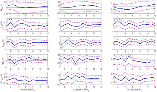
The theoretical model (McDonald & Siegel, 1986) regarding the reaction of investment shows that the firm will take a wait and see strategy in order to avoid the negative uncertainty shock. However, this only interprets the partial investment behaviors in China. To investigate the US uncertainty shock on China’s investment, Yan and An (2020) conclude that SOEs’ investment increases but POEs’ investment declines. However, our impulse response findings indicate that economic policy uncertainty makes the pattern of China’s investments (no matter SOEs or POEs) more complex. A possible explanation is that economic policy will guide banks loans to these firms directly, especially bank loans to the private-owned enterprises.

When we proceed to explore how time-stamped uncertainty shocks affect bank loans in the short-, medium-, and long-term. We find that bank loans with different maturities behave similarly in response to economic policy uncertainty as investments in China. Actually, once we realize that bank loans are the major external financing for most enterprises in China, it is straightforward to understand the similar patterns of bank loans and investments in response to economic policy uncertainty shock. Finally, we turn to analyze how the interest rate responds to economic policy uncertainty shock. Different from the quarterly VAR model, the responses of interest rate to the first- and second-month economic policy uncertainty shocks are positive but negative to the third-month economic policy uncertainty shock. In other words, the PBC in China will decline the interest rate after two months when the PBC recognizes the occurrence of economic policy uncertainty shock, rather than only increase immediately the interest rate as shown by the quarterly VAR model. Consider the institutional background and how the PBC taking a loose stance works for reducing the adverse effects of economic policy uncertainty, the MF-VAR model can better capture the response of interest to EPU shock. In sum, impulse responses in the MF-VAR provide richer implications than in the quarterly VAR.

To further compare the explanatory power of MF-VAR with quarterly VAR, we further report the contribution of movements in core China’s variables is explained by economic policy uncertainty in three months. Table 3 presents the results of variance decomposition. Here, we only consider empirical results when the prediction horizon is 12. For the total contribution of uncertainty shock (${\sum }_{i=1}^3{\mathrm{EPU}}_i$), uncertainty shock plays a much larger role in explaining the fluctuations in China’s investments and bank loans. Specifically, total contribution of uncertainty shock (${\sum }_{i=1}^3{\mathrm{EPU}}_i$) is 14.280%, 16.264%, 39.101%, and 13.213%, respectively. Therefore, economic policy uncertainty has a nonnegligible role in accounting for the fluctuations in China’s investments and bank loans rather than the negligible role shown by the quarterly VAR. This suggests that aggregating monthly economic policy uncertainty into a quarterly level underestimates the influence of economic policy uncertainty in shaping China’s macroeconomy. In the meanwhile, the MF-VAR analysis allows us to uncover more details in investigating the importance of time-stamped uncertainty shock in explaining the long-run forecast error variance. An intriguing result we find is uncertainty shock in the 2^nd month (${\mathrm{EPU}}_2$) accounts for a larger percentage of aggregate fluctuations in the POEs’ investment and medium- and long-term bank loans, and uncertainty shock in the 3^rd month (${\mathrm{EPU}}_3$) contributes to a larger percentage of aggregate movements in the SOEs’ investment and short-term bank loans.

Table 3. Forecast error variance decomposition of MF-VAR(4).

Decomposition of ${\mathrm{R}}_{\mathrm{IB}}$
Horizons	${\mathrm{EPU}}_1$	${\mathrm{EPU}}_2$	${\mathrm{EPU}}_3$	${\sum }_{i=1}^3{\mathrm{EPU}}_i$	${\mathrm{R}}_{\mathrm{IB}}$
$\mathrm{h}=4$	3.224	1.848	3.499	8.570	77.998
$\mathrm{h}=8$	2.246	5.149	4.375	11.770	60.408
$\mathrm{h}=12$	2.531	7.397	4.506	14.434	55.131
Decomposition of ${\mathrm{BL}}_{\mathrm{S}}$
Horizons	${\mathrm{EPU}}_1$	${\mathrm{EPU}}_2$	${\mathrm{EPU}}_3$	${\sum }_{i=1}^3{\mathrm{EPU}}_i$	${\mathrm{R}}_{\mathrm{IB}}$
$\mathrm{h}=4$	4.634	2.407	18.212	25.253	7.371
$\mathrm{h}=8$	8.027	6.117	24.414	38.558	6.017
$\mathrm{h}=12$	8.906	5.973	24.136	39.015	6.050
Decomposition of ${\mathrm{BL}}_{\mathrm{ML}}$
Horizons	${\mathrm{EPU}}_1$	${\mathrm{EPU}}_2$	${\mathrm{EPU}}_3$	${\sum }_{i=1}^3{\mathrm{EPU}}_i$	${\mathrm{R}}_{\mathrm{IB}}$
$\mathrm{h}=4$	1.556	2.208	2.414	6.179	1.512
$\mathrm{h}=8$	2.294	6.450	4.075	12.819	1.463
$\mathrm{h}=12$	2.314	6.974	3.926	13.213	4.248
Decomposition of ${\mathrm{I}}_{\mathrm{SOE}}$
Horizons	${\mathrm{EPU}}_1$	${\mathrm{EPU}}_2$	${\mathrm{EPU}}_3$	${\sum }_{i=1}^3{\mathrm{EPU}}_i$	${\mathrm{R}}_{\mathrm{IB}}$
$\mathrm{h}=4$	3.844	1.720	6.075	11.640	4.864
$\mathrm{h}=8$	4.890	2.712	6.204	13.806	5.729
$\mathrm{h}=12$	4.837	2.964	6.480	14.280	6.617
Decomposition of ${\mathrm{I}}_{\mathrm{POE}}$
Horizons	${\mathrm{EPU}}_1$	${\mathrm{EPU}}_2$	${\mathrm{EPU}}_3$	${\sum }_{i=1}^3{\mathrm{EPU}}_i$	${\mathrm{R}}_{\mathrm{IB}}$
$\mathrm{h}=4$	4.068	7.596	3.724	15.389	7.9626
$\mathrm{h}=8$	3.491	6.986	4.679	15.155	10.765
$\mathrm{h}=12$	3.255	6.943	6.067	16.264	11.308

Notes: All values in percentage. We conduct the forecast error variance decomposition of each series at prediction horizons of $\mathrm{h}=4,\mathrm{ }8,\mathrm{ }12$ quarters.

Source: Authors' calculations.

4.3. Decomposition of SOEs’ investment

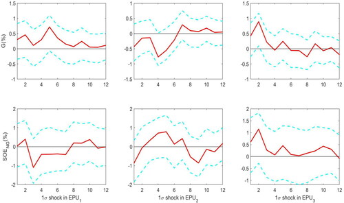
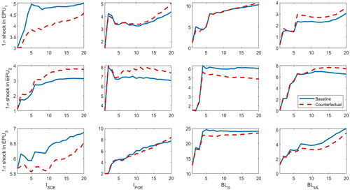
Follow Chang et al. (2016), the SOEs’ investment has two components: one part from the government investment injecting to the state-owned enterprises because the SOEs bear partial social service and achieve specific policy goals; another part is the SOEs’ investment which behaves like a real enterprise to maximize the investment income. Consistently, to comprehensively understand the responses of state-owned enterprise investment to economic policy uncertainty shock, we further decompose the SOEs’ investment into two parts, one part belongs to the government investment to the SOEs (we denote it as G), another part only belongs to the state-owned enterprise investment excluding the government investment (we denote it as ${\mathrm{SOE}}_{\mathrm{NG}}$).

By comparing the panel in the first row and the panel in the second row in Figure 4, it is straightforward to conclude that the responses of two components have the same direction, no matter positive in 1^st and 3^rd months or negative in 2^nd month. Consider the following accounting equation, ${\mathrm{I}}_{\mathrm{SOE}}{=\mathrm{G}+\mathrm{SOE}}_{\mathrm{NG}},$ then according to the definition of the impulse response, we finally have $\frac{{\partial \mathrm{I}}_{\mathrm{SOE}}}{\partial \mathrm{EPU}}=\frac{\partial \mathrm{G}}{\partial \mathrm{EPU}}+\frac{{\partial \mathrm{SOE}}_{\mathrm{NG}}}{\partial \mathrm{EPU}},$ this implies that the effects of economic policy uncertainty on SOEs’ investment are strengthened due to the existence of the injection of the government investment into state-owned enterprises.

Figure 4. Impulse responses based on mixed frequency VAR(4): Decomposition of SOEs’ investment.

Notes: This figure presents impulse responses of two components of state-owned enterprises’ (SOEs) investment based on the MF-VAR(4) of the monthly economic policy uncertainty shock, as well as quarterly interest rate shock. The solid line plots the impulse response for quarterly horizons (1 to 12). The dashed lines plot the corresponding 68% bootstrapped confidence intervals.

Source: Authors' calculations.

4.4. The role of interest rate: A counterfactual analysis

To reduce the negative impact of policy uncertainty shocks, the PBC seeks to implement a series of financial policies, including monetary policy, credit policy, and regulatory policy, to keep China’s economic growth resilient and stable. The second-quarter Monetary Policy Report in 2019 states that “From the beginning of 2019, following the policy arrangements of the CPC Central Committee and the State Council, the PBC pursued a sound monetary policy, deepened financial supply-side structural reforms, and maintained steady credit growth…… the PBC remained focused on its mandate while effectively handling the internal and external uncertainties….A series of monetary-policy instruments……was employed to keep liquidity at a reasonable and adequate level so as to guide the downward movement of interest rates.” Therefore, a natural question to ask in this context is to what extent economic policy uncertainty through the interest rate transmission channel contributes to aggregate fluctuations in China.

To address this issue, we should close the indirect propagation channel of economic policy uncertainty through interest rate and further conduct a counterfactual exercise by means of variance decomposition. Refer to Akıncı (2013), there is no need to re-estimate the MF-VAR model, we only need to modify the MF-VAR system given in Eq.(2)(2) $$\underset{{\mathbf{Y}}_{\mathrm{t}}}{\underbrace{\left[\begin{array}{c} {\mathrm{EPU}}_{1\mathrm{t}}\\ {\mathrm{EPU}}_{2\mathrm{t}}\\ {\mathrm{EPU}}_{3\mathrm{t}}\\ {\mathrm{R}}_{\mathrm{IBt}}\\ {\mathrm{BL}}_{\mathrm{St}}\\ {\mathrm{BL}}_{\mathrm{MLt}}\\ {\mathrm{I}}_{\mathrm{SOEt}}\\ {\mathrm{I}}_{\mathrm{POEt}}\end{array}\right]}}=\sum _{\mathrm{k}=1}^4\underset{{\mathbf{B}}_{\mathrm{k}}}{\underbrace{\left[\begin{array}{c}{\mathbf{B}}_{1\mathrm{k}}\\ {\mathbf{B}}_{2\mathrm{k}}\\ {\mathbf{B}}_{3\mathrm{k}}\\ {\mathbf{B}}_{4\mathrm{k}}\\ {\mathbf{B}}_{5\mathrm{k}}\\ {\mathbf{B}}_{6\mathrm{k}}\\ {\mathbf{B}}_{7\mathrm{k}}\\ {\mathbf{B}}_{8\mathrm{k}}\end{array}\right]}}\underset{{\mathbf{Y}}_{\mathrm{t}-\mathrm{k}}}{\underbrace{\left[\begin{array}{c} {\mathrm{EPU}}_{1\mathrm{t}-\mathrm{k}}\\ {\mathrm{EPU}}_{2\mathrm{t}-\mathrm{k}}\\ {\mathrm{EPU}}_{3\mathrm{t}-\mathrm{k}}\\ {\mathrm{R}}_{\mathrm{IBt}-\mathrm{k}}\\ {\mathrm{BL}}_{\mathrm{St}-\mathrm{k}}\\ {\mathrm{BL}}_{\mathrm{MLt}-\mathrm{k}}\\ {\mathrm{I}}_{\mathrm{SOEt}-\mathrm{k}}\\ {\mathrm{I}}_{\mathrm{POEt}-\mathrm{k}}\end{array}\right]}}+\underset{{\mathbf{\epsilon }}_{\mathrm{t}}}{\underbrace{\left[\begin{array}{c} {\mathrm{\epsilon }}_{1\mathrm{t}}\\ {\mathrm{\epsilon }}_{2\mathrm{t}}\\ {\mathrm{\epsilon }}_{3\mathrm{t}}\\ {\mathrm{\epsilon }}_{4\mathrm{t}}\\ {\mathrm{\epsilon }}_{5\mathrm{t}}\\ {\mathrm{\epsilon }}_{6\mathrm{t}}\\ {\mathrm{\epsilon }}_{7\mathrm{t}}\\ {\mathrm{\epsilon }}_{8\mathrm{t}}\end{array}\right]}}$$(2) such that the economic policy uncertainty doesn’t affect other variables through interest equation as follows: (3) $${\mathrm{R}}_{\mathrm{IBt}}={\sum }_{\mathrm{k}=1}^4\left[\sum _{\mathrm{j}=1}^3{\mathrm{b}}_{4\mathrm{j}}\mathrm{ }{\mathrm{EPU}}_{\mathrm{jt}-\mathrm{k}}+{\mathrm{b}}_{44}{\mathrm{R}}_{\mathrm{IBt}-\mathrm{k}}+{\mathrm{b}}_{45}{\mathrm{I}}_{\mathrm{SOEt}-\mathrm{k}}+{\mathrm{b}}_{46}{\mathrm{I}}_{\mathrm{POEt}-\mathrm{k}}+{{\mathrm{b}}_{47}\mathrm{B}\mathrm{L}}_{\mathrm{St}-\mathrm{k}}+{{\mathrm{b}}_{48}\mathrm{B}\mathrm{L}}_{\mathrm{MLt}-\mathrm{k}}\right]+{\mathrm{\epsilon }}_{4\mathrm{t}}$$(3)

Empirically, the monthly economic policy uncertainty (${\mathrm{EPU}}_{\mathrm{jt}-\mathrm{k}})$ in equation (3)(3) $${\mathrm{R}}_{\mathrm{IBt}}={\sum }_{\mathrm{k}=1}^4\left[\sum _{\mathrm{j}=1}^3{\mathrm{b}}_{4\mathrm{j}}\mathrm{ }{\mathrm{EPU}}_{\mathrm{jt}-\mathrm{k}}+{\mathrm{b}}_{44}{\mathrm{R}}_{\mathrm{IBt}-\mathrm{k}}+{\mathrm{b}}_{45}{\mathrm{I}}_{\mathrm{SOEt}-\mathrm{k}}+{\mathrm{b}}_{46}{\mathrm{I}}_{\mathrm{POEt}-\mathrm{k}}+{{\mathrm{b}}_{47}\mathrm{B}\mathrm{L}}_{\mathrm{St}-\mathrm{k}}+{{\mathrm{b}}_{48}\mathrm{B}\mathrm{L}}_{\mathrm{MLt}-\mathrm{k}}\right]+{\mathrm{\epsilon }}_{4\mathrm{t}}$$(3) is modified by setting to zero coefficients on ${\mathrm{b}}_{4\mathrm{j}},$ namely, ${\mathrm{b}}_{4\mathrm{j}}=0,$ where $\mathrm{j}\in \{1,2,3\}.$ Then we can compute the impulse response functions and perform variance decomposition based on the modified VAR system.

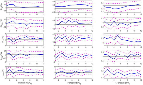
The variance decomposition of the counterfactual analysis by removing the indirect transmission channel of economic policy uncertainty via interest rate is shown in Figure 5. When we shut off the response of the interest rate to economic policy uncertainty, the forecast error variance presents richer patterns. First, economic policy uncertainty in the 3^rd month accounts for smaller movements in investments and bank loans. Second, economic policy uncertainty in the 1^st and 2^nd months will increase the contribution to fluctuations in six cases⁸ and decrease the contribution to movements in two cases. Therefore, we conclude that the impact of economic policy uncertainty on China’s investments and bank loans are alleviated when the interest rate channel exists. In other words, the change in the interest rate will eliminate partially adverse effects from economic policy uncertainty.

Figure 5. Forecast error variance decomposition of MF-VAR(4): A counterfactual analysis without interest rate channel.

Notes: The solid lines depict the fraction of the variance of the k-quarter ahead forecasting error explained EPU shock. The dashed line shows the fraction of the variance of the k-quarter under the counterfactual analysis in which the interbank rate is assumed not to respond directly to variations in the economic policy uncertainty.

Source: Authors' calculations.

4.5. Does trade policy uncertainty matter?

This section investigates the impact of trade policy uncertainty, another concept is closely related to economic policy uncertainty in China, especially after the US-China trade war started in 2018. This trade conflict brings more uncertainty to the world economy and prolongs the recovery of the global economy. Go back to the panel in Figure 1, we find common trends of economic policy uncertainty and trade policy uncertainty after 2015. The close linkage between domestic investments and bank loans attributes to the important trade position of China in the global economy as the largest exporter and second largest importer in the world. As discussed before, the trade policy uncertainty index developed by Davis et al. (2019) is shorter than the economic policy uncertainty index and spans from 2000M1 to 2017M12.

Figure 6 plots the impulse responses of investments and bank loans to 1σ trade policy uncertainty shock. By comparing economic policy uncertainty shock and trade policy uncertainty shock, the difference lies in the responses of medium- and long-term bank loans to 1st and 2nd months trade policy uncertainty shock. The responses of medium- and long-bank loans to 1st and 2nd months economic policy uncertainty is around zero in the first period and then becomes positive. However, the trade policy uncertainty in the 1st and 2nd months will generate significantly positive impacts on ${\mathrm{BL}}_{\mathrm{ML}}.$ Table 4 reports the forecast error variance decomposition of FM-VAR(4) with trade policy uncertainty. We confirm that the contribution of trade policy uncertainty to fluctuations in investments and bank loans are very close. Basically, trade policy uncertainty will have a similar influence on China’s investments and bank loans as economic policy uncertainty. We shouldn’t be surprised by these empirical results because there is a high correlation (0.548) relationship between EPU and TPU in our sample period.

Figure 6. Impulse responses based on mixed frequency VAR(4): Trade policy uncertainty.

Notes: This figure presents the impulse responses based on the MF-VAR(4) of monthly trade policy uncertainty shock, as well as quarterly interest rate shock. The solid line plots the impulse response for quarterly horizons (1 to 12). The dashed lines plot the corresponding 68% bootstrapped confidence intervals.

Source: Authors' calculations.

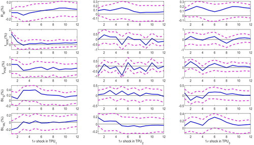
Table 4. Forecast error variance decomposition of MF-VAR(4): Trade policy uncertainty.

Decomposition of ${\mathrm{R}}_{\mathrm{IB}}$
Horizons	${\mathrm{TPU}}_1$	${\mathrm{TPU}}_2$	${\mathrm{TPU}}_3$	${\sum }_{i=1}^3{\mathrm{TPU}}_i$	${\mathrm{R}}_{\mathrm{IB}}$
$\mathrm{h}=4$	10.833	0.198	4.073	15.104	71.264
$\mathrm{h}=8$	7.917	5.131	3.945	16.992	52.763
$\mathrm{h}=12$	7.597	6.549	4.467	18.612	46.150
Decomposition of ${\mathrm{BL}}_{\mathrm{S}}$
Horizons	${\mathrm{TPU}}_1$	${\mathrm{TPU}}_2$	${\mathrm{TPU}}_3$	${\sum }_{i=1}^3{\mathrm{TPU}}_i$	${\mathrm{R}}_{\mathrm{IB}}$
$\mathrm{h}=4$	6.758	2.105	7.579	16.442	25.706
$\mathrm{h}=8$	14.580	1.979	10.565	27.124	20.411
$\mathrm{h}=12$	14.414	1.962	9.622	25.998	18.810
Decomposition of ${\mathrm{BL}}_{\mathrm{ML}}$
Horizons	${\mathrm{TPU}}_1$	${\mathrm{TPU}}_2$	${\mathrm{TPU}}_3$	${\sum }_{i=1}^3{\mathrm{TPU}}_i$	${\mathrm{R}}_{\mathrm{IB}}$
$\mathrm{h}=4$	10.067	9.961	1.606	21.634	2.493
$\mathrm{h}=8$	8.739	12.896	1.953	23.588	3.059
$\mathrm{h}=12$	7.949	12.454	2.507	22.910	6.414
Decomposition of ${\mathrm{I}}_{\mathrm{SOE}}$
Horizons	${\mathrm{TPU}}_1$	${\mathrm{TPU}}_2$	${\mathrm{TPU}}_3$	${\sum }_{i=1}^3{\mathrm{TPU}}_i$	${\mathrm{R}}_{\mathrm{IB}}$
$\mathrm{h}=4$	2.493	3.437	4.315	10.245	3.932
$\mathrm{h}=8$	3.370	4.286	5.795	13.451	4.034
$\mathrm{h}=12$	3.301	4.636	6.068	14.005	4.129
Decomposition of ${\mathrm{I}}_{\mathrm{POE}}$
Horizons	${\mathrm{TPU}}_1$	${\mathrm{TPU}}_2$	${\mathrm{TPU}}_3$	${\sum }_{i=1}^3{\mathrm{TPU}}_i$	${\mathrm{R}}_{\mathrm{IB}}$
$\mathrm{h}=4$	2.940	8.907	7.704	19.551	9.334
$\mathrm{h}=8$	2.554	8.190	8.271	19.016	9.362
$\mathrm{h}=12$	2.378	7.528	7.825	17.731	9.808

Notes: All values in percentage. We conduct the forecast error variance decomposition of each series at prediction horizons $\mathrm{h}=4,\mathrm{ }8,\mathrm{ }12$ quarters.

Source: Authors' calculations.

5. Robustness checks

In this section, we briefly illustrate and perform a series of robustness tests to confirm our findings in the benchmark model. This section considers the results of robustness based on (i) a specific proxy used for China’s economic policy uncertainty; (ii) real vs. nominal variables; (iii) a different lag order; (iv) a different Cholesky order to satisfy the identification assumption of the VAR system.

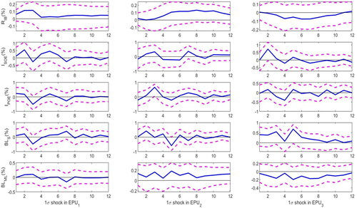
(i) In the first robustness, we consider a different proxy of economic policy uncertainty constructed by Davis et al. (2019). The correlation coefficient between this EPU proxy and BBD-type EPU is 0.656, so we conjecture that the impulse responses of China’s investments and bank loans to this proxy of EPU will generate similar patterns as our benchmark model. As depicted in Figure 7 of robustness 1, our main findings are robust to different measures of economic policy uncertainty. Also, the MF-VAR model indicates richer conclusions as explained above. (ii) In the second robustness, we attempt to answer whether the nominal or real variables have different responses to economic policy uncertainty shock. Refer to Chang et al. (2016), to get the real variables of investments and bank loans, the investments of SOEs and POEs are deflated by the investment price index, and total bank loans with different maturities are deflated by the implicit GDP deflator. Figure 8 presents the impulse responses of real variables rather than nominal variables to economic policy uncertainty shock. Once again, the impulse responses of investments and bank loans are unchanged irrespective of economic policy uncertainty shock at different time points.

Figure 7. Robustness 1: Proxy Variable of Policy Uncertainty.

Notes: This figure uses the economic policy uncertainty measured by Davis et al. (2019) as an alternative proxy of policy uncertainty to conduct the robustness check. The solid line plots the impulse response for quarterly horizons (1 to 12). The dashed lines plot the corresponding 68% bootstrapped confidence intervals.

Source: Authors' calculations.

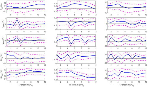
Figure 8. Robustness 2: Real vs Nominal Variables.

Notes: This figure uses the price indexes to deflate the nominal variables in the benchmark model to conduct the robustness check. The solid line plots the impulse response for quarterly horizons (1 to 12). The dashed lines plot the corresponding 68% bootstrapped confidence intervals.

Source: Authors' calculations.

The next two robustness tests consider the model specification. (iii) In our benchmark model, we set the lag length to 4 to eliminate the seasonal factors as Motegi and Sadahiro (2018). In the robustness, we set the lag length to 2 to analyze whether the results are robust to different lag orders. Figure 9 plots the impulse responses to economic policy uncertainty when the lag order is set to 2. (iv) In the last robustness, we attempt to check whether the order of core variables in the Cholesky decomposition is important. In the benchmark model, we impose the order that ${\mathrm{R}}_{\mathrm{IB}}{\to \mathrm{BL}}_{\mathrm{S}}\to {\mathrm{BL}}_{\mathrm{ML}}\to {\mathrm{I}}_{\mathrm{SOE}}\to {\mathrm{I}}_{\mathrm{POE}},$ but we turn it to be ${\mathrm{R}}_{\mathrm{IB}}\to {\mathrm{I}}_{\mathrm{POE}}\to {\mathrm{I}}_{\mathrm{SOE}}{\to {\mathrm{BL}}_{\mathrm{ML}}\to \mathrm{BL}}_{\mathrm{S}}$ in our robustness. Figure 10 graphs the impulse responses to economic policy uncertainty when the new Cholesky order is imposed. Overall, we can observe that the impulse response results corresponding to the robustness checks are quite similar to the baseline results, both qualitatively and quantitatively.

Figure 9. Robustness 3: Selection of Lag Order.

Notes: This figure sets the lag order as 2 rather than 4 to conduct the robustness check. The solid line plots the impulse response for quarterly horizons (1 to 12). The dashed lines plot the corresponding 68% bootstrapped confidence intervals.

Source: Authors' calculations.

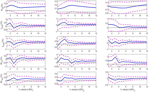
Figure 10. Robustness 4: Choice of the Cholesky Order.

Notes: This figure sets a different Cholesky order. The solid line plots the impulse response for quarterly horizons (1 to 12). The dashed lines plot the corresponding 68% bootstrapped confidence intervals.

Source: Authors' calculations.

6. Conclusions

This paper first investigates the impact of high-frequency China’s economic policy uncertainty shock on SOEs’ and POEs’ investment, as well as short-, medium- and long-term bank loans by employing the mixed-frequency vector autoregression framework. Impulse response analysis suggests that time-stamped China’s economic policy uncertainty generates partly heterogeneous impacts on China’s investments and bank loans, which is likely to be covered by using the traditional quarterly VAR model. Variance decomposition analysis finds that aggregating monthly economic policy uncertainty into a quarterly level underestimates the influence of economic policy uncertainty in shaping China’s macroeconomy.

By further decomposing the SOEs’ investment, we reveal that the effects of economic policy uncertainty on SOEs’ investment are strengthened due to the existence of the injection of the government investment into state-owned enterprises. A counterfactual experiment is also conducted to address the following issue that to what extent economic policy uncertainty through the interest rate transmission channel contributes to aggregate fluctuations in China. The counterfactual analysis shows that the impacts of economic policy uncertainty on China’s investments and bank loans are alleviated when the interest rate channel exists. In addition, by introducing trade policy uncertainty in light of the recently intensified US-China trade conflict, we conclude that trade policy uncertainty will have a similar influence on China’s investments and bank loans as economic policy uncertainty.

These findings are robust to a range of robustness checks, including a specific proxy used for China’s economic policy uncertainty; real vs nominal variables; a different lag order; a different Cholesky order to satisfy the identification assumption of the VAR system.

Our analysis results have two important implications for policymakers. First, China’s central bank has a relatively delayed response to adjust the interest rate in response to economic policy uncertainty, which recalls the issue of whether the PBC should become an independent central bank. Second, the recent trade conflict between China and the United States giving rise to higher policy uncertainty should be paid enough attention by the Chinese policymakers.

Acknowledgments

I would like to thank all anonymous referees for their valuable suggestions.

Disclosure statement

No potential conflict of interest was declared by the authors.

Additional information

Funding

This study was funded by National Social Sciences Funds (20BTJ015).

Notes

1 State-owned enterprises (SOEs) in China refer to firms owned by all citizens of China and controlled by central and local governments. Usually, the objectives of SOEs go beyond profits, including resources, employment, and foreign policy. In China, some SOEs controlled by the central government (e.g., State Grid Corporation of China) and most SOEs controlled by the local governments are nonlisted firms. Private-owned enterprises (POEs) refer to firms excluding state-owned enterprises.

2 Baker et al. (2019) point out that the recent rise in trade policy uncertainty threatens to become the new normal and trade policy uncertainty further generates negative effects on firm-level and macroeconomic performance.

3 Although Liu and Zhang (2015) show that EPU leads to significant increases in China’s stock market volatility, we should be cautious about the results of Liu and Zhang (2015). Liu and Zhang (2015) only cover the period from January 2, 1996 to June 24, 2013, which belongs to the periods that there is a close comovement between EPU and stock market volatility. When we turn to focus on recent periods, such as the US-China trade conflict, it is straightforward to find that the correlation between EPU and stock market volatility decreases substantially.

4 Similarly, based on the evidence of the US, Caggiano et al. (2014) estimate a smoothed transition VAR and find that the effects of uncertainty shocks are asymmetric over the business cycle in that unemployment and inflation react more to uncertainty shocks during recessions than they do during expansions.

5 By performing the stationary test, including the Augmented Dickey-Fuller (ADF) and Phillips-Perron (PP) unit root test, we take logarithm for all variables except the interest rate. We use the level of interbank offered rate as the interest rate. Also, we keep the log-level of EPU but use the log-difference of SOEs’ investment, POEs’ investment, short-term bank loans, as well as, medium- and long-bank loans.

6 As Motegi and Sadahiro (2018) point out, MF-VAR is primarily used for a small ratio of sampling frequencies, e.g., monthly/quarterly, rather than large ratio, e.g., daily/quarterly. Consider the EPU index is measured at a monthly frequency, therefore, the MF-VAR model satisfies our need for the subsequent analysis.

7 Davis et al. (2019) also construct the monthly trade policy uncertainty (TPU) index for China runs from January 2000 to the present. We rely on this index to analyze the impact of trade policy uncertainty. We should notice that Huang and Luk (2020) also construct a broad economic policy uncertainty in China on the basis of 114 newspapers published in mainland China. However, the length of EPU constructed by Huang and Luk (2020) starts from January 2000, therefore, this index is too short for our benchmark analysis.

8 Including Figures (1,2), (1,3), (1,4), (2,1), (2,2), and (2,4).

References

- Akıncı, Ö. (2013). Global financial conditions, country spreads and macroeconomic fluctuations in emerging countries. Journal of International Economics, 91(2), 358–371. https://doi.org/https://doi.org/10.1016/j.jinteco.2013.07.005
- Baker, S. R., Bloom, N., & Davis, S. J. (2016). Measuring economic policy uncertainty. The Quarterly Journal of Economics, 131(4), 1593–1636. https://doi.org/https://doi.org/10.1093/qje/qjw024
- Baker, S., Bloom, N., & Davis, S. (2019). The extraordinary rise in trade policy uncertainty. Reading, 19, 21.
- Bernanke, B. S. (1983). Irreversibility, uncertainty, and cyclical investment. The Quarterly Journal of Economics, 98(1), 85–106. https://doi.org/https://doi.org/10.2307/1885568
- Bloom, N. (2009). The impact of uncertainty shocks. Econometrica, 77(3), 623–685.
- Bloom, N. (2014). Fluctuations in uncertainty. Journal of Economic Perspectives, 28(2), 153–176. https://doi.org/https://doi.org/10.1257/jep.28.2.153
- Caggiano, G., Castelnuovo, E., & Groshenny, N. (2014). Uncertainty shocks and unemployment dynamics in US recessions. Journal of Monetary Economics, 67, 78–92.
- Chang, C., Chen, K., Waggoner, D. F., & Zha, T. (2016). Trends and cycles in China’s macroeconomy. NBER Macroeconomics Annual, 30(1), 1–84. https://doi.org/https://doi.org/10.1086/685949
- Chen, J., Jiang, F., & Tong, G. (2017). Economic policy uncertainty in China and stock market expected returns. Accounting & Finance, 57(5), 1265–1286. https://doi.org/https://doi.org/10.1111/acfi.12338
- Chen, K., & Zha, T. (2018). Macroeconomic effects of China's financial policies (No. w25222). National Bureau of Economic Research.
- Choi, S., & Shim, M. (2019). Financial vs. Policy uncertainty in emerging market economies. Open Economies Review, 30(2), 297–318. https://doi.org/https://doi.org/10.1007/s11079-018-9509-9
- Chong, T. T. L., & Liu, W. (2017). The roadmap of interest rate liberalisation in China. Economic and Political Studies, 5(4), 421–440. https://doi.org/https://doi.org/10.1080/20954816.2017.1384614
- Davis, S. J., Liu, D., & Sheng, X. S. (2019). Economic policy uncertainty in China since 1946: the view from mainland newspapers. Working paper.
- Ferrara, L., & Guérin, P. (2018). What are the macroeconomic effects of high‐frequency uncertainty shocks? Journal of Applied Econometrics, 33(5), 662–679. https://doi.org/https://doi.org/10.1002/jae.2624
- Fontaine, I., Didier, L., & Razafindravaosolonirina, J. (2017). Foreign policy uncertainty shocks and US macroeconomic activity: Evidence from China. Economics Letters, 155, 121–125. https://doi.org/https://doi.org/10.1016/j.econlet.2017.03.034
- Fontaine, I., Razafindravaosolonirina, J., & Didier, L. (2018). Chinese policy uncertainty shocks and the world macroeconomy: Evidence from STVAR. China Economic Review, 51, 1–19. https://doi.org/https://doi.org/10.1016/j.chieco.2018.04.008
- Ghysels, E. (2016). Macroeconomics and the reality of mixed frequency data. Journal of Econometrics, 193(2), 294–314. https://doi.org/https://doi.org/10.1016/j.jeconom.2016.04.008
- Han, L., Qi, M., & Yin, L. (2016). Macroeconomic policy uncertainty shocks on the Chinese economy: a GVAR analysis. Applied Economics, 48(51), 4907–4921. https://doi.org/https://doi.org/10.1080/00036846.2016.1167828
- Huang, Y., & Luk, P. (2020). Measuring economic policy uncertainty in China. China Economic Review, 59, 101367. https://doi.org/https://doi.org/10.1016/j.chieco.2019.101367
- Li, X. M. (2017). New evidence on economic policy uncertainty and equity premium. Pacific-Basin Finance Journal, 46, 41–56. https://doi.org/https://doi.org/10.1016/j.pacfin.2017.08.005
- Li, Z., & Luo, S. (2019). Is risk shock a key factor driving business cycles in China? The BE Journal of Macroeconomics, 19(1), 1–18.
- Lin, J. Y., Cai, F., & Li, Z. (1998). Competition, policy burdens, and state-owned enterprise reform. The American Economic Review, 88(2), 422–427.
- Liu, G., & Zhang, C. (2020). Economic policy uncertainty and firms' investment and financing decisions in China. China Economic Review, 63, 101279. https://doi.org/https://doi.org/10.1016/j.chieco.2019.02.007
- Liu, L., & Zhang, T. (2015). Economic policy uncertainty and stock market volatility. Finance Research Letters, 15, 99–105. https://doi.org/https://doi.org/10.1016/j.frl.2015.08.009
- McDonald, R., & Siegel, D. (1986). The value of waiting to invest. The Quarterly Journal of Economics, 101(4), 707–727. https://doi.org/https://doi.org/10.2307/1884175
- Motegi, K., & Sadahiro, A. (2018). Sluggish private investment in Japan’s Lost Decade: Mixed frequency vector autoregression approach. The North American Journal of Economics and Finance, 43, 118–128. https://doi.org/https://doi.org/10.1016/j.najef.2017.10.009
- Pastor, L., & Veronesi, P. (2017). Explaining the puzzle of high policy uncertainty and low market volatility. VOX Column, 25.
- Wang, Y., Chen, C. R., & Huang, Y. S. (2014). Economic policy uncertainty and corporate investment: Evidence from China. Pacific-Basin Finance Journal, 26, 227–243. https://doi.org/https://doi.org/10.1016/j.pacfin.2013.12.008
- Wu, J., Zhang, J., Wu, Y., & Kong, D. (2019). When to go abroad: economic policy uncertainty and Chinese firms’ overseas investment. Accounting and Finance.
- Yan, M., & An, Z. (2020). The Impacts of High-frequency US Uncertainty Shocks on China’s Investments and bank Loans: Evidence from mixed-frequency VAR. Applied Economics Letters, forthcoming.
- Zhang, G., Han, J., Pan, Z., & Huang, H. (2015). Economic policy uncertainty and capital structure choice: Evidence from China. Economic Systems, 39(3), 439–457. https://doi.org/https://doi.org/10.1016/j.ecosys.2015.06.003