Theoretical and experimental evidence on stock market volatilities: a two-phase flow model

Abstract

The volume–volatility relationship usually ignores possible effects of stock shares. This article proposes a two-phase flow model assuming that capital and stock flows determine stock price and return volatility. Computational simulations suggest that monodirectional capital or stock flows and collective flows exert different effects on stock return volatilities. Considering the impact of stock flows, the positive relationship between capital and return volatility is no longer guaranteed. The inflow of capital and the outflow of stock increase stock price similarly; but exhibit completely different effects on stock return volatilities. A persistent stock inflow (outflow) reduces (intensifies) return volatilities, whereas a monodirectional persistent capital outflow has no such effect. When capital and stock flows’ velocities satisfy critical values determined by the initial state of the market, the market enlargement accompanied with increasing stock and capital shows no impact on market stability because of stable return volatilities. Otherwise, stock flows drive return volatilities with stronger effects than capital flows. Further experimental studies that simulate the real stock market through a trading system provide strong evidence supporting the two-phase flow model. Given similar driving forces of capital and stock flows, the interaction of them should be considered in constructing investment strategies and setting policies.

Keywords:

• capital
• stock
• volume–volatility
• two-phase flow model
• experiment
• econophysics

JEL:

• C92
• G12
• G17
• G40

1. Introduction

The volume–volatility relationship has been the centre of financial studies, but its nature has not been yet fully examined. Trading volume and stock return volatility in financial markets typically, but not always, move in tandem (Bollerslev et al., 2018), which inspires the central role of trading volume in pricing financial assets. However, the reasons for the occasionally moderate inverse movements of volume and return volatility are unrevealed (e.g., Pisedtasalasai & Gunasekarage, 2007; Okan et al., 2009). Most findings regarding the relationship between volume–volatility ignore the role of the numbers of stocks. The effect of volume, particularly in terms of money, is hardly possible to be independent of the number of stocks being traded in the market. For instance, both capital and stock are likely to flow into the market during the period of Initial Public Offerings (I.P.O.s). Nevertheless, minimal studies research the effect of stock flows on return volatilities. The conflicting empirical evidence surrounding the precise relationship between trading volume and stock return volatility has added fuel to this debate paving the way for considering other possible driving factors. This article attempts to analyse whether the traditionally argued positive volume–volatility relationship is affected by changes in stocks through investigating the effects of stock and capital flows on return volatilities, which, to the best of our knowledge, has not been revealed in existent literature.

It is difficult to divide the effect of trading volumes in terms of money and stock shares on the stock return volatility from one to another in the empirical study because both factors are driven by certain common forces. Additional rights issues, I.P.O.s and hot money inflow are likely to appear simultaneously when the macro-economy is strong. It has been recognised that financial markets are more volatile in the real-world data than in standard models (Shiller, 1981; Adam et al., 2016), and the interaction between capital and stock flows is one possible reason. Thereby, different from previous literature, this article resorts to the experimental method to produce evidence for the effect of capital and stock flows on stock return volatilities. We simulate the real market through a trading system which allows us to adjust the trading scenario in which only capital or stock changes. Meanwhile, inspired by the vigorous development of econophysics, we propose a two-phase flow model in which capital and stock flows determine stock price and return volatility. The capital and stocks in the market change over time, thus generating time-varying average price of stock and return volatility.

This study provides a number of theoretical and experimental contributions. First, we propose a theoretical model that attempts to explain the stock return volatility. The two-phase flow model considers the interaction of capital and stock, thus showing that the effect of capital on stock return volatility depends on the amount of stocks. Second, based on the theoretical model, we simulate the formation of stock price and return volatility for many cases. Specifically, we simulate monodirectional capital flow, monodirectional stock flow and collective flows of two factors in the same and opposite directions, respectively. We find significantly different effects of capital and stock flows on the stock market. Capital and stock flows exhibit similar effects in driving stock price; however, their impacts on return volatilities are completely different. Stock flows appear to dominate capital flows in driving return volatilities. Thus, simulation results provide a possible explanation for different volume–volatility relationships reported in distinct markets. Finally, experimental studies which simulate the real trading market are conducted to produce evidence for the effects of capital and stock flows on the financial market, particularly on return volatilities. The real stock market is driven by multiple factors that is hardly possible to be controlled. Compared with the computer simulation of multi-agents models, the experimental method resorts to human beings, which considers the emotional effects of agents that cannot be simulated by computers. Thus, experimental methods capture the real reflection of investors to changes occurred in the stock market. Overall, both theoretical and experimental results suggest that the interaction between capital and stock shares validates in forming the volume–volatility relationship, in which changes in stocks are driving forces. Further research and policies considering such linkage well benefit the stability of the financial market and investing strategies.

This study proceeds as follows. Section 2 is a literature review. Section 3 proposes a theoretical model that attempts to explain the roles of capital and stocks in affecting return volatilities and provides corresponding computational simulations. Section 4 illustrates an experiment that simulate the real market to test the effect of stock and capital flows on return volatilities, and Section 5 concludes this article.

2. Literature review

Capital flows exert significant effects on stock markets, particularly on market volatilities. As demonstrated by Bennett and Sias (2001), money flow appears to provide investors with information regarding future returns and can to certain extent explain cross-sectional variation in future returns. Nonetheless, minimal studies test the effect of capital flows on stock volatilities directly. Generally, relating literature concerns capital flows from three perspectives: trading volume, hot money, and equity funds.

The measurement of trading volume is quite different in the literature, including the size of trading volume measured by the amount of capital and the number of traded stocks. Thereby, the effect of trading volume on stock volatility should be classified into two aspects: the size of trading volume, i.e., volume in terms of money and the number of trading stocks. Unfortunately, most existent literature fails to distinguish between them. The research regarding the size of trading volume is closely related to our study because the effective capital injected into the stock market is exactly the amount of money traded. A large number of studies support a positive relationship between trading volume and return volatilities. Karpoff (1987) summarises some theoretical explanations on the relation between price changes and trading volume in financial markets, i.e., the moisture of distribution hypothesis (M.D.H.; Epps & Epps, 1976), the Sequential Information Arrival Hypothesis (S.I.A.H.; Copeland & Galai, 1983), and the life-cycle trading (Pfleiderer1984). The M.D.H. model postulates that the stock returns are conditionally normal with a variance which is based upon the intensity of information arrivals. Meanwhile, trading volume and stock prices are determined by information flows because of trades induced by information arrivals. Thus, stock return volatility and trading volume are positively interlinked through information flows. The M.D.H. model has been widely adopted in empirical studies to explain the volume–volatility relationship in stock and futures markets, e.g., Kartsaklas (2018), Naik et al. (2018) and Bohl and Stefan (2020). The S.I.A.H. argues that trading volume as a proxy of information helps to predict return volatilities because investors receive new information sequentially. Tseng et al. (2015), Shen et al. (2018) and Yu et al. (2019) among many others find positive evidence supporting the S.I.A.H. in explaining volume–volatility relationships in stock markets. Two more recent models have been proposed. Admati and Pfleiderer (1988) consider the asymmetric information between traders and suggest that concentrated-trading patterns arise endogenously as a result of the strategic behaviour of liquidity traders and informed traders. The patterns of trading volume and price variability in intraday transactions can therefore be explained. Scheinkman and Xiong (2003) and Banerjee and Kremer (2010) develop a disagreement model in which investors disagree about the interpretation of public information. Consequently, a positive correlation between volume and stock return volatility generates because of the impacts of public information.

Meanwhile, a large quantity of empirical studies find evidence supporting a close relationship between trading volume and stock return volatility for the past decades. Li and Wu (2006) show that the positive relationship between stock return volatility and trading volume is primarily driven by the informed component of trading according to the M.D.H. However, when the information flow is controlled, the return volatility is negatively related to trading volume. He and Velu (2014) develop a multi-asset M.D.H. model in which stock returns and volatility are assumed to jointly depend on a latent information flow and empirically demonstrate such prediction. Do et al. (2014) find an unambiguously positive and significant relationship between the realised volatility and the trading volume which is represented by the number of trades, which supports heterogeneous beliefs among investors. Pevzner et al. (2015) report increases in both trading volume and stock return variance during the earnings announcement period by researching across 25 countries. Paital and Sharma (2016) find a positive relationship between return volatility and trading volume, which favours the S.I.A.H. over M.D.H. for the Indian stock market. By contrast, Naik et al. (2018) support the M.D.H. based upon evidence from South Africa. The relationships between intraday trading volume and stock volatilities in other markets such as futures markets are frequently investigated by recent studies, e.g., Balcilar et al. (2017), Bollerslev et al. (2018), Kartsaklas (2018), Ma et al. (2018) and Koubaa and Slim (2019). Studies regarding the liquidity–volatility relationship also contribute to the understanding of the volume–volatility relationship because liquidity is particularly determined by trading volume (Chordia et al., 2000; Będowska-Sójka & Kliber, 2019). Nevertheless, based on the M.D.H., Bose and Rahman (2015) find that contemporaneous trading volume contributes little to the removal of significant heteroscedasticity effects in Bangladesh. Thampanya et al. (2020) also note that trading volume is not the most important factor in affecting stock return volatilities. They find that trading volume affects emerging market volatility more than developed market volatility, whereas the proportion of young firms plays a notable role. Thereby, it is reasonable to infer that the number of stock shares is a possible reason for discrepancies in the volume–volatility relationship.

Massive amounts of speculative funds, or ‘hot money’, flow from one country to another to earn a short-term profit, thus leading to controversial effects on the stock market. However, one can reasonably speculate that increases in hot money in a country will unavoidably raise the capital in the stock market. Thereby, the research of the relation between hot money and stock markets is closely related to our topic. Many studies claim a significant effect of hot money on stock prices and volatilities, particularly in emerging markets such as Mexico and India (Chari & Kehoe, 2003). More recent studies focus on the effect of hot money on the Chinese stock market. Guo and Huang (2010) indicate that hot money has accelerated stock volatilities in China. Wei et al. (2018) imply that the Chinese stock market is not driven by hot money, and vice versa. However, hot money has a significant positive impact on the long-term volatility of the Chinese stock market. Nevertheless, Waqas et al. (2015) suggest that whether hot money drives Chinese stock volatility remains unclear.

Another strand of literature that closely related to our research investigates how mutual fund flows affect stock markets. Beaumont et al. (2008) use the aggregate money flows in and out of domestically-oriented U.S. mutual funds to measure individual investor sentiments and find that such sentiment has a significant impact on stock volatilities. The result agrees with Lee et al. (2002). However, Cao et al. (2008) document a different impact which supports a negative relation between the inflow of aggregate mutual fund and stock volatilities. Lee et al. (2015) support an evident relationship among stock volatilities, market returns, and the aggregate equity fund flows in the U.S., but not in Asian countries. Nevertheless, Goh and Sapian (2017) report that the stock volatility is positively related to net equity flows of local investors whilst is negatively related to that of foreign investors in the Malaysian market. Evidence regarding significant relations between fund flows and stock markets are also demonstrated in other countries such as Australia, Japan and China (Watson & Wickramanayake, 2012; Alexakis et al., 2013; Wang, 2014).

For studies investigating the effect of stock flows on markets, most focus on the role of I.P.O. To the best of our knowledge, there is no research studying the number of stocks actually traded in the market in analysing market volatilities. A possible reason may be that it is difficult to separate the effect of stock flows given numerous factors influencing stock markets. Schwert (2002) analyses the relation of the unusual Nasdaq volatility to the hot I.P.O. market in 1998 and 1999 and concludes that the technology I.P.O. appears to explain the unusual volatility best. Pástor and Veronesi, (2005) suggest that I.P.O. waves are accompanied by changes in stock returns, and Pettway et al. (2008) and Loughran and Mcdonald (2013) argue that I.P.O.s affect stock return volatilities. Despite that I.P.O. and additional rights issues that enlarge stock flows are expected to exert significant effects on stock markets, insufficient evidence has been exploited theoretically and empirically.

Meanwhile, an emerging area, i.e., the econophysics, has been widely explored in explaining complex non-linear phenomena in financial markets. The pioneering work of Mantegna and Stanley (1995) demonstrates that the Standard & Poor's 500 can be described by a non-Gaussian process of Lévy stable process. Following Mantegna and Stanley (1995), many micro-models have been proposed to explain the long-term correlation of volatility and the associated wave aggregation behaviour. Lux and Marchesi (1999) describe a multi-agent model of financial markets which supports that scaling emerges from mutual interactions of participants. Wang and Wang (2012) and Yu and Wang (2012) propose and promote financial pricing models which are developed by the stochastic lattice percolation theory (a random network). Hong and Wang (2014) develop a financial agent-based time series model based on the Potts model and investigate volatilities of financial time series through simulation and empirical tests. More related studies such as Mike and Farmer (2008) and Fang and Wang (2012), among many others, support that financial analysis based on physical models captures the properties of stock markets.

Finally, turning to the experimental linkage among trading volume, capital and stock returns, a limited number of studies provide certain evidence. For instance, Zhang et al. (2014) utilise a similar simulated stock trading system with the one adopted in this study and find that stock returns are negatively related to the trading volume in unilaterally price-rising markets. However, they also note that such a relationship disappears in unilaterally price-falling markets. Additionally, the above study investigates the effects of gender and personality on the relationship between trading volume and stock returns, which are confirmed by many studies using the real stock market data, e.g., Richards and Willows (2018) and Zhang et al. (2019). Thus, the study of Zhang et al. (2014) provides solid support to the method of simulation from the real stock markets. More related studies resort to computational simulations of an artificial stock market, e.g., Krichene and El-Aroui (2018a) and Lee and Lee (2020). In these studies, the developed stock market is usually order-driven and populated by heterogeneous agents to simulate the real stock market (Krichene & El-Aroui, 2018b). Despite its similar mechanism with the real stock market, artificial markets can never simulate the emotion and behaviour changes of individual investors.

3. Theoretical model and simulation

3.1. The two-phase flow model of stock market

The one-dimensional flow controlling volume model of physical fluid mechanics assumes that fluid continues to flow into and out of the container. When the fluid fills the container, the upper of the container wall will exert certain pressure on the fluid, thus controlling the volume of the container and speeding up the liquid flow rate. In the stock market, it is practically impossible that stock prices maintain unchanged when the amounts of capital and stock vary. Therefore, we set a ‘non-control volume model’, i.e., the liquid level in the container changes with different flow speeds of the fluid. In the stock market, traders keep buying and selling stocks, thus making money flow in and out of the market. Meanwhile, there are I.P.O.s, secondary offerings and delisting that will change the total number of shares in the stock market. Consequently, money and stocks flow in and out of the stock market every moment as fluid flow. Similarly, the stock price works as the liquid level in the container, which varies and fluctuates with the flows of money and stocks in the market. We propose a two-phase flow model to explain the fluctuation of stock prices according to the significant similarity between stock markets and hydromechanics. We assume that money and the share of stocks in the stock market change over time, i.e., m(t) and s(t). Correspondingly, the average price of stock changes over time, i.e., p(t). The symbols of s(0), m(0) and p(0) represent the number of stocks, capital quantity and stock price in the initial state, respectively. The initial average stock price is: (1) $$p\left(0\right)=\frac{m\left(0\right)}{s\left(0\right)}$$(1)

To explain the relationship among the average price and number of stocks and capital quantity, we further apply six assumptions to the models as follows. First, money and stocks can be freely circulated and converted without any constrains at any time, which means that the stock market has sufficient liquidity. Second, the flow of money can be totally converted to the market value. Third, the trading of stocks occurs continuously, which means that the capital flow is continuous and dm/dt exists. Four, the stock flow caused by I.P.O. and delisting is continuous and ds/dt exists. Five, the average stock price changes continuously and dp/dt exists. Finally, the average stock price is determined by the total capital quantity and the number of stocks, i.e., p(t)=m(t)/s(t). Thereby, the stock price at time t is determined as follows: (2) $$p\left(t\right)=\frac{m\left(0\right)+\Delta m}{s\left(0\right)+\Delta s}$$(2) where $\Delta m$ and $\Delta s$ denote changes in $m$ and $s,$ respectively. Correspondingly, $\Delta p$ is the change in the average stock price during the period $\Delta t$ which is determined by: (3) $$\Delta p=\frac{m\left(0\right)+\Delta m}{s\left(0\right)+\Delta s}-\frac{m\left(0\right)}{s\left(0\right)}$$(3)

Given that $p\left(\mathrm{t}\right),$ $m\left(t\right),$ and $s\left(t\right)$ are continuously differentiable, Eq. (3)(3) $$\Delta p=\frac{m\left(0\right)+\Delta m}{s\left(0\right)+\Delta s}-\frac{m\left(0\right)}{s\left(0\right)}$$(3) means that: (4) $$v_p\left(t\right)=\frac{1}{s\left(0\right)}{v}_m\left(t\right)-\frac{m\left(0\right)}{s^2\left(0\right)}{v}_s\left(t\right)$$(4) where $v_p(t),$ $v_m(t)$ and $v_s(t)$ are the velocities of changes in the average stock price, capital flow and stock flow, respectively. We can obtain the following equation through integral: (5) $${\int }_o^T{v}_p\left(t\right)dt=\frac{1}{s\left(0\right)}{\int }_o^T{v}_m\left(t\right)dt-\frac{m\left(0\right)}{s^2\left(0\right)}{\int }_o^T{v}_s\left(t\right)dt$$(5)

According to Eq. (5)(5) $${\int }_o^T{v}_p\left(t\right)dt=\frac{1}{s\left(0\right)}{\int }_o^T{v}_m\left(t\right)dt-\frac{m\left(0\right)}{s^2\left(0\right)}{\int }_o^T{v}_s\left(t\right)dt$$(5) , increases and decreases in stock prices are the same as the capital flow, but opposite to the stock flow. Therefore, the average stock price increases when capital flows into the market while stocks flow out of it. By contrast, an inflow of stocks and outflow of capital will decrease the average stock price. However, when capital and stocks move in the same direction, the average price of stock depends on the balance of two factors. For example, when both capital and stocks flow into the market and the former dominated the latter, the average stock price will rise, and vice versa. Furthermore, when the capital flow exceeds stock flow to a certain extent, effects of the number of stocks can be ignored, which means that the average stock price changes in line with that of capital flow. By contrast, when the number of stocks dominates the capital flow, the former leads to negative changes in the average stock price.

We obtain the average stock price and corresponding return volatility according to Eq. (5)(5) $${\int }_o^T{v}_p\left(t\right)dt=\frac{1}{s\left(0\right)}{\int }_o^T{v}_m\left(t\right)dt-\frac{m\left(0\right)}{s^2\left(0\right)}{\int }_o^T{v}_s\left(t\right)dt$$(5) . (6) $$p\left(t\right)=p\left(0\right)+\frac{1}{s\left(0\right)}{\int }_o^T{v}_m\left(t\right)dt-\frac{m\left(0\right)}{s^2\left(0\right)}{\int }_o^T{v}_s\left(t\right)dt$$(6) (7) $$\sigma =\sqrt{nD\left(\mathit{ln}\frac{m\left(0\right)s\left(0\right)+s\left(0\right){\int }_o^T{v}_m\left(t\right)dt-m\left(0\right){\int }_o^T{v}_s\left(t\right)dt}{m\left(0\right)s\left(0\right)+s\left(0\right){\int }_o^{T-1}{v}_m\left(t\right)dt-m\left(0\right){\int }_o^{T-1}{v}_s\left(t\right)dt}\right)}$$(7)

The average potential stock price and return volatility are determined by capital quantity, the number of stocks, velocities of capital and stock flows. Particularly, in a short time period, when the number of stocks and the velocity of stock flow are likely to maintain the same, the effects of capital flow on stock prices and return volatility can be predicted.

3.2. Simulation

We proceed to simulate the effects of capital and stock flows on the stock return volatility under constraint conditions. Specifically, we study four cases: the number of stocks mains unchanged (Panel A in Table 1), the capital quantity remains (Panel B in Table 1), capital and stock flow in the opposite directions (Panel C in Table 1), and capital and stock flow in or out simultaneously for the rest three cases with specific velocities (Panels D–F in Table 1). The settings of initial capital and stocks are based on the Chinese stock market, and $v_m(t)$ and $v_s(t)$ refer to the daily velocities. We simulate the changes in stock return volatility for 200 steps, each step contains 22 simulations, corresponding to 22 trading days. Thus, the horizontal axis refers to the time at the horizon of month, and the vertical axis denotes stock return volatilities.

Table 1. Parameters settings for the simulation of the (potential) market volatility.

Group Number	$\mathrm{m}(0)$ (trillion)	$\mathrm{s}(0)$ (trillion)	$v_m(t)$	$v_s(t)$
Panel A: monodirectional capital flow
1	${10}^2$	${10}^1$	${10}^{-2}$	$0$
2	${10}^2$	${10}^1$	${-10}^{-2}$	$0$
Panel B: monodirectional stock flow
3	${10}^2$	${10}^1$	0	${10}^{-3}$
4	${10}^2$	${10}^1$	0	$-{10}^{-3}$
Panel C: capital and stock flow in opposite directions
5	${10}^2$	${10}^1$	${10}^{-2}$	${-10}^{-3}$
6	${10}^2$	${10}^1$	${-10}^{-2}$	${10}^{-3}$
Panel D: capital and stock flows in the same direction: $v_m(t)/v_s(t)$=m(0)/s(0)
7	${10}^2$	${10}^1$	${10}^{-2}$	${10}^{-3}$
8	${10}^2$	${10}^1$	${-10}^{-2}$	$-{10}^{-3}$
Panel E: capital and stock flows in the same direction: $v_m(t)/v_s(t)$<m(0)/s(0)
9	${10}^2$	${10}^1$	$9^{-2}$	${10}^{-3}$
10	${10}^2$	${10}^1$	${-9}^{-2}$	$-{10}^{-3}$
Panel F: capital and stock flows in the same direction: $v_m(t)/v_s(t)$>m(0)/s(0)
11	${10}^2$	${10}^1$	${11}^{-2}$	${10}^{-3}$
12	${10}^2$	${10}^1$	${-11}^{-2}$	$-{10}^{-3}$

Notes: The initial values of capital and stock shares are based on the Chinese stock market. $v_m(t)$ and $v_s(t)$ are velocities of capital and stock flows, respectively. s(0) and m(0) represent the number of stocks and capital quantity in the initial state.

Source: The Authors.

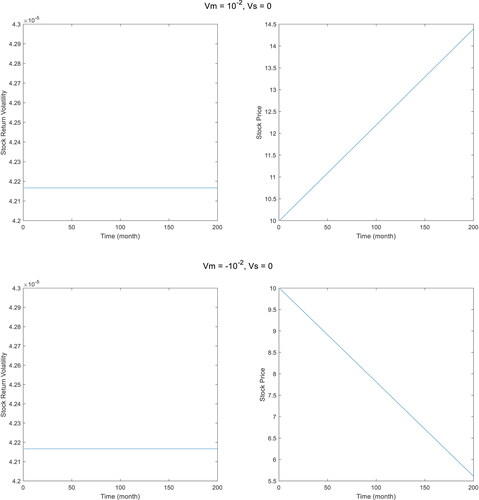
First, we simulate the potential stock return volatility when the number of stocks maintains unchanged, i.e., the velocity of stock flow is zero. As explained by the M.D.H. and S.I.A.H., trading volume and stock return volatility are contemporaneously positively related because of their joint dependence on the common factor of the flow of new information in the market (Paital & Sharma, 2016). Inflows of capital thus should stimulate a larger return volatility, and the equilibrium price should be immediately established. According to Panel A in Table 1 and Figure 1, the potential average price increases when $v_m(t)$ is positive, thus meaning that the inflow of capital rises stock prices, in line with the expectation of Eq. (6)(6) $$p\left(t\right)=p\left(0\right)+\frac{1}{s\left(0\right)}{\int }_o^T{v}_m\left(t\right)dt-\frac{m\left(0\right)}{s^2\left(0\right)}{\int }_o^T{v}_s\left(t\right)dt$$(6) and M.D.H. and S.I.A.H. However, as can be observed in Figure 1, the potential stock return volatility shows little fluctuation. By contrast, a sudden inflow of capital increases the stock return volatility compared with when the market is in a stable state (which is expected to show no fluctuation). A constant inflow of capital shows no impact on the market stability over a longer-term horizon of 200 months, because the potential stock return volatility maintains approximately the same over the simulation period. Similarly, an outflow of capital triggers a sudden increase in the stock return volatility, but shows no persistent effect. Meanwhile, a capital outflow results in a lower stock price as expected. Thus, the simulation indicates that capital inflows with a time-invariant velocity are not necessarily positively related to increases in return volatilities.

Figure 1. The simulation results of stock return volatility and average stock price (Panel A, monodirectional capital flow). Source: The Authors.

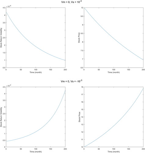
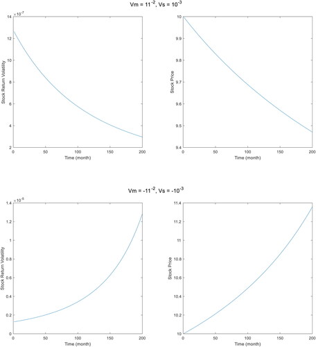
Then, we simulate the stock return volatility and stock price when the velocity of capital flow equals zero, i.e.,$\mathrm{}{v}_m(t)=0,$ meaning that the capital quantity maintains unchanged. The settings of parameters are summarised in Panel B of Table 1. As shown in Figure 2, as expected, the inflow and outflow of stocks exhibit distinct effects on the trend of stock price. Specifically, when the capital quantity maintains the same, a constant inflow of stock results in a logarithmic form decrease of stock price. Thereby, the return volatility decreases over time in a similar logarithmic form. By contrast, the stock price increases in a quasi-exponential form when stock flows out of the market at a constant speed, and thus generates a quasi-exponentially increased stock return volatility. In other words, an outflow of stock impacts the stock return stability significantly, and a constant outflow will cause even more drastic fluctuations over a longer-term horizon. Comparing Figures 1 and 2, we can find that stock flows appear to exert much more significant effects on the stock return volatility than capital flows. The results of following simulations provide further evidence.

Figure 2. The simulation results of stock return volatility and average stock price (Panel B, monodirectional stock flow). Source: The Authors.

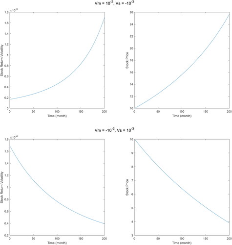
The above discussion regards the unilateral flow of stock or capital. In the following simulations, we analyse the simultaneous movements of capital and stock in the same and opposite directions, respectively. As summarised in Panel C and Figure 3, the stock price and stock return volatility under the inflow of capital and outflow of stock show similar patterns with the case of monodirectional stock outflow in Figure 2, but with significantly stronger effects. Consequently, the price and stock return volatility at the end of the simulation period are much greater. Meanwhile, the outflow of capital and inflow of stock generate similar results with the case of monodirectional stock inflow. Clearly, the results show that the opposite movements of capital and stock strength the effects on stock return volatility of each other; but appear to indicate that the effects of stock flow dominate that of capital flow. Through comparing the stock return volatilities in Figures 1–3, it is easy to find that the opposite movement of capital strengthens the effect of stock flow on stock return volatility, particularly when the capital flows out. Such results are consistent with the theoretical model in which the increase in capital plays a similar role as the decrease in stocks.

Figure 3. The simulation results of stock return volatility and average stock price (Panel C, flows in opposite directions). Source: The Authors.

According to Eq. (6)(6) $$p\left(t\right)=p\left(0\right)+\frac{1}{s\left(0\right)}{\int }_o^T{v}_m\left(t\right)dt-\frac{m\left(0\right)}{s^2\left(0\right)}{\int }_o^T{v}_s\left(t\right)dt$$(6) , when the changes of capital and stock flows are constrained to $v_m\left(t\right)/v_s\left(t\right)=\mathrm{m}/\mathrm{s},$ the stock price should maintain unchanged over time. As a consequence, the stock return volatility should be zero, thus indicating that the market is in a stable state. Therefore, the simulation under co-movements of capital and stock flows in the same direction is further categorised into three situations: $v_m\left(t\right)/v_s\left(t\right)=\mathrm{m}/\mathrm{s}$ (Panle D), $v_m\left(t\right)/v_s\left(t\right)<\mathrm{m}/\mathrm{s}$ (Panel E), and $v_m\left(t\right)/v_s\left(t\right)>\mathrm{m}/\mathrm{s}$ (Panel F). Figure 4 displays the results of potential stock return volatility and stock price when the stock and capital flow in the same direction and satisfies $v_m\left(t\right)/v_s\left(t\right)=\mathrm{m}/\mathrm{s}.$ As expected, the stock price maintains unchanged and the stock return volatility remains zero.

Figure 4. The simulation results of stock return volatility and average stock price (Panel D, $v_m\left(t\right)/v_s\left(t\right)=\mathrm{m}(0)/\mathrm{s}(0)$). Source: The Authors.

When considering different absolute velocities of stock and capital flows, the results are quite different. Figures 5 and 6 report the results of Panels E and F, respectively. In Panel E, $v_m\left(t\right)/v_s\left(t\right)<\mathrm{m}/\mathrm{s},$ meaning that the velocity ratio of capital flow and stock flow is smaller than the initial capital stock ratio. As shown in Figure 5, the movements of stock price and return volatility are quite different from the monodirectional flow cases of Figures 1 and 2. The collective inflow of capital and stock results in increases in stock prices, but decreases stock return volatility. Concerning the effects on stock return volatility, the collective inflow of capital and stock is similar with the monodirectional inflow of stock (Figure 2), but with comparatively weaker impact. By contrast, the collective outflow of capital and stock decreases stock prices, but increases stock return volatility. Again, the collective outflow of capital and stock exhibits a similar but weaker effect on stock return volatility comparing with the monodirectional outflow of stock (Figure 2). Thus, the results show that the flows of capital weaken the effect of stock flows. We can summarise that when the capital flows with a small enough velocity, the stock flow in the same direction drives the market.

Figure 5. The simulation results of stock return volatility and average stock price (Panel E, $v_m\left(t\right)/v_s\left(t\right)<\mathrm{m}(0)/\mathrm{s}(0)$). Source: The Authors.

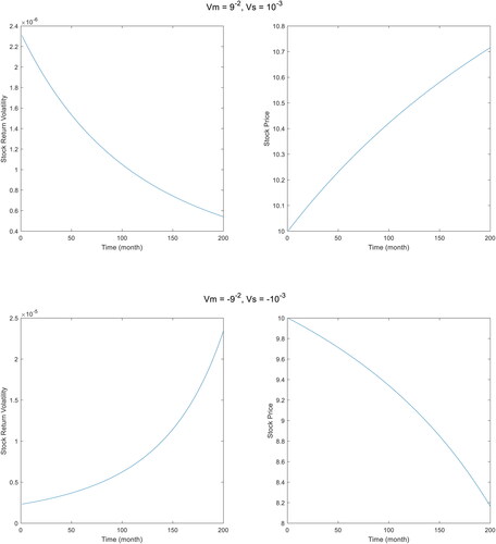
Figure 6. The simulation results of stock return volatility and average stock price (Panel E, $v_m\left(t\right)/v_s\left(t\right)>\mathrm{m}/\mathrm{s}$). Source: The Authors.

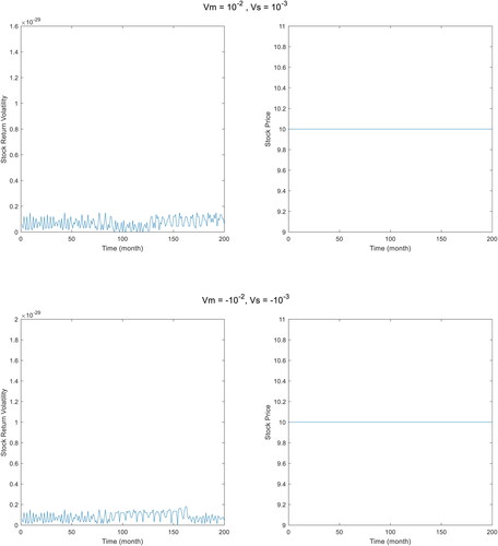
Finally, when stock and capital flow in the same direction and satisfy $v_m\left(t\right)/v_s\left(t\right)>\mathrm{m}/\mathrm{s},$ results are different. Figure 6 displays the simulation results of Panel F. When the inflow velocity of capital is large enough ($v_m\left(t\right)>v_s\left(t\right)\mathrm{m}/\mathrm{s}$), the collective inflow of stock and capital results in decreased stock price and lowers the stock return volatility. By contrast, the collective outflow of stock and capital increases stock price and stock return volatility. By comparing with the results in Figure 2 and Figure 5, we can find stock flow drives the market even when the capital velocity is quite large ($\left|v_m\left(t\right)\right|>\left|v_s\left(t\right)\right|\mathrm{*}\mathrm{m}/\mathrm{s}$). A monodirectional capital inflow has little effect on stock return volatility, whereas a monodirectional stock inflow decreases stock return volatility. When both capital and stock flow into the market with an inconstant velocity, which assures that $v_m\left(t\right)/v_s\left(t\right)\ne \mathrm{m}/\mathrm{s},$ the stock return volatility decreases. Thereby, the stock flow is again demonstrated to be the main driver of stock return volatility instead of capital flows. Furthermore, the results indicate that when stock flows into the market, an influx of capital can help to stabilise the market through decreasing stock return volatilities. Nevertheless, if stock flows out of the market, the following capital loss may intensify the market fluctuation. Overall, the stock return volatility mainly depends on changes in stocks, whereas the interaction of stock and capital affects stock price.

The simulation results suggest that stock and capital flows exert significant effects on the return volatility and stock price. We can draw several conclusions from the above discussions. First, monodirectional capital inflow (outflow) increases (decreases) the stock price, but exerts little effect on the long-term stock return volatility. Second, monodirectional stock inflow (outflow) decreases (increases) stock price and return volatility. Third, the opposite flow of capital intensifies the effect of stock flows. Fourth, the collective inflow or outflow of capital and stock affects stock return volatility significantly, but with specific effects determined by the relative flow velocity of them. Specifically, when the velocities of stock and capital flows maintain relatively fixed to the initial capital stock ratio, the market stays stable with comparatively unchanged stock return volatility.

4. Behavioural finance experiments and analysis

4.1. Behavioural finance experiments

We use the experimental method to produce evidence for the effect of capital and stock changes on stock return volatilities. Ever since the pioneering work of Smith et al. (1988), using experimental methods to study behaviours in stock markets has been widely accepted. For instance, investigating I.P.O. underpricing (Haruvy et al., 2014) and asset bubbles with short-selling mechanism (Haruvy & Noussair, 2006), dividend mechanism (Cheung & Coleman, 2014) and information asymmetry (Ghosh et al., 2015), etc. In our experiments, we simulate the real market through a trading system which allows us to adjust the trading scenario. The real stock market is driven by multiple factors that is hardly possible to be controlled. Compared with the computer simulation of multi-agents models, the experimental method resorts to human beings, which considers emotional effects of agents that cannot be simulated by computers. Thus, the experimental method can to a better extent capture the real reflection of investors to changes occurred in the stock market and produce unique evidence that empirical tests can hardly achieve.

4.1.1. Trading platform

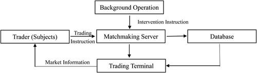
The platform developed by the School of Economics and Management at the University of Science & Technology Beijing (U.S.T.B.) provides a stock simulation trading system. This platform enables approximately 200 agents to participate in the trade simultaneously using the hardware (servers and computers) and software (stock simulation trading system) supported by the financial engineering laboratory of U.S.T.B. The experimental platform contains four parts as shown in Figure 7. First, the trading terminal, which provides the subjects with main functions of pending orders, withdrawing orders, entrusting record query, querying transaction record, querying asset, showing real-time price, displaying time-sharing chart, etc. Second, the matchmaking server following the rules of price priority and time priority. The matchmaking server will match the pending orders of the subjects in both directions and give real-time feedbacks on the transaction interface. Third, the background operation, through which the experimental designer controls the opening and closing of trading, stock types and handling fees. Meanwhile, we can change the number of stocks and capital of subjects, control the market trend and release news through the background operation. Finally, the database. During the experiment, the platform records the transaction quantity, transaction price and the total amount of capital at each moment according to the instructions of the subjects, and automatically forms the commission and transaction records. Therefore, the experimental platform provides a continuous two-way auction system, which highly simulates the real market and furnishes real-time transaction data.

Figure 7. Trading platform of the experiment. Source: The Authors.

4.1.2. Trading system

The transaction price is determined by the entrustment order, which adopts the continuous auction mode, price priority and time priority rules. The trading system is a ‘T + 0′ delivery and settlement system, which means that the settlement and delivery take place immediately after the transaction occurs. To settle means to exchange the shares (stocks) for the cash and to deliver means reverse operations. This system improves the market liquidity to better simulate the continuous trading in a real market. Besides, there is no handling charge for transactions between buyers and sellers because every experiment is strictly restricted to 20 minutes, followed by a five minute break to avoid the resistance psychology and aversion emotion of subjects. Meanwhile, to prevent the merging and truncation problems that will affect data integrity, there is no limit on the rise and fall of stock prices in the experiments. We set the limit of the price falling margin to be 99.9% because the price cannot be zero. To ensure the trading activity, each experiment trades one unique stock, and the price and fundamental information are determined by specific experiment requirements.

4.1.3. Experimental investment situation

Due to the experimental time limit and the main research objective, there are no dividends and financial statements of the traded stock despite that these can be implemented through the platform. Two groups of experiments are designed: the effects of capital flow on stock return volatilities, and the effects of stock flows. The 265 participants in this experiment are students in the selected investment course provided by the U.S.T.B. The students came from 16 universities majoring in specialised subjects. The students were permitted to communicate with one another and to trade online at the same time. Each experiment lasted 20 minutes, and there was a five-minute break between each experiment. We employed standard psychological methods which would not cause physical or psychological damage. We followed the guide of the Chinese Ethics Committee of Registering Clinical Trials and received the approval of Student Affairs, which was responsible for the safety of students and was a formal organisation at the U.S.T.B. Before the experiments, we informed the students that the course score is positively related to their personal stock returns. Such scoring mechanism encourages subjects to actively and seriously involve in the trading experiment to strive for higher test scores. As found by Moore and Taylor (2007), credit system and incentive system are similar to experiments regarding students as the main experimental subject.

In the first group of experiments, we tested the capital flow on stock return volatilities. Three groups of subjects were tested according to the settings in Table 2. For these two groups, three experiments were conducted and each experiment lasted 20 minutes. There was a five-minute break between each two experiments. During the above experiments, the number of stock shares was maintained the same, and we increased the capital quantity of traders through the background operation to simulate the capital flow in real markets. Each of the subjects in each of the experimental pre-openings was assigned with 10,000 shares of stock. After the opening, buyers and sellers traded freely for 20 minutes. Then, the system was shut down for five minutes between each of the two fields.

Table 2. Experiment results.

	Experiment	Capital (Thousand RMB)	Stock (Share)	Stock Return Volatility	Equilibrium Price
Panel A: monodirectional capital flow
Group 1 (185 participants)	1	200	10000	0.0017	23.75
	2	800	10000	0.0070	49.67
	3	1600	10000	0.0077	193.22
Group 2 (80 participants)	1	200	10000	0.0012	21.47
	2	800	10000	0.0030	45.82
	3	1600	10000	0.0105	158.28
Panel B: monodirectional stock flow
Group 1 (185 participants)	1	400	1000	0.0434	118.29
	2	400	5000	0.0084	70.62
	3	400	10000	0.0039	27.25
Group 2 (80 participants)	1	400	1000	0.0510	148.24
	2	400	5000	0.0186	77.93
	3	400	10000	0.0036	29.38

Source: The Authors.

The second group of experiment tested the effect of monodirectional stock flow on stock return volatilities. Similar to the above design, each of the subjects in each of the experimental pre-openings was assigned 400,000 R.M.B. cash in their personal capital account. Buyers and sellers traded freely for 20 minutes and the trading was closed for five minutes during which the number of stocks will be changed according to Table 2.

4.2. Data analysis

First, we analyse the effect of capital flow on stock return volatilities. Figure 8 shows the stock price movements of three experiments for Group 1 which are generated by the participants’ own behaviour without any interference. It shows that in the early few minutes in each experiment, the stock price rose because of a large amount of buy deals, but after reaching a peak, it fluctuated until the end of the experiments. Generally, stock prices for each experiment evolved to comparatively stable prices without any manipulation. The results for Group 2 show similar patterns.¹ We then calculate the stock return volatility of each experiment and summarise the results in Panel A of Table 2. According to Figure 8 and Table 2, the comparative equilibrium stock price² is approximately 23.6, and the corresponding stock return volatility is 0.0017 for experiment 1, for which 200,000 R.M.B. and 10,000 stock shares were injected into each participant’s account before the trading. After the first 20 minutes trading (experiment 1), 600,000 R.M.B. capital was injected into each participant’s account during the five minutes’ break. Then, the second experiment with enlarged capital generated an equilibrium price of about 50 and a stock return volatility of 0.0070, which are significantly larger than that in experiment 1. Similarly, after the second 20 minutes’ trading, another 800,000 R.M.B. was injected, and the equilibrium stock price and return volatility further increased. Such experimental results agree with the simulation results of Panel A, in which a sudden increase in capital rises the market price and return volatility instantly. To verify the reliability of our experiments, we resort to another group of participants using the same experiment design. As shown in Table 2, the injection of capital intensifies the stock return volatility, thus supporting the results of Group 1 and simulation results of Panel A in Table 1.

Figure 8. Stock prices of three experiments in Group 1. Source: The Authors.

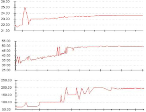
According to Figure 8, the increase in capital results in a larger capital stock ratio, which further affects the equilibrium stock price and return volatility. Actually, these experiments simulate the process of stock bubble and tumble caused by hot money. With the increase of capital, the effect of capital inflow on stock price was enlarged. Extreme changes in capital flow may generate more significant effects on the market stability.

Panel B in Table 2 summarises the experimental results of the effect of monodirectional stock flow on the return volatility. In the initial experiment for Group 1, each participant has 400,000 R.M.B. capital and 1,000 stock shares. The stock return volatility for experiment 1 is 0.0434. When we injected 4,000 shares of stock into the market after the first trading period, the stock return volatility decreased significantly from 0.0434 to 0.0084. Meanwhile, the equilibrium stock price also declined. Similar results generate for Group 2. When another 5,000 shares of stock were injected after the market reached a comparative stable state, the stock price and return volatility further declined. Although we simulate the process of issuing additional rights, the effect of I.P.O. is expected to have the same effect because both operations lead to increases in trading stocks in the real market. The experiment results agree with Figure 2 in which monodirectional inflow of stock decreases the stock price and return volatility. Meanwhile, comparing the results for Group 1 in Panels A and B, we also find evidence supporting that stock flows exhibit stronger effects in reducing stock return volatilities than capital flows.

In this article, we did not simulate the outflow of capital and stock and the collective flows of two factors because of limited resource. However, our simulation and experiment results provide strong evidence supporting that capital and stock flows affect the stock price and return volatility. In most empirical analysis, the powerful effect of capital, particularly the effective capital that is actively traded in the market was to a certain extent ignored. Our results indicate that both capital and stock quantities are important factors in studying and forecasting the performance of stock markets.

5. Conclusion

Modest fluctuations ensure the stock market liquidity and improve effective allocation of resources. By contrast, excessive volatility undermines the transmission mechanism of stock prices which reduces the market efficiency and aggravates losses. Therefore, more knowledge about the generation of the financial market volatility is of significance for investors and market regulators. Most previous literature focus on the volume–volatility relationship without considering the possible effect of stock flows. However, similar driving forces behind capital and stock indicate that the ignorance of stock flows may lead to biased results. Many studies find a positive linkage between trading volume in terms of money and stock return volatility, whereas divergent movements or insignificant correlations between them also exist in some markets. For instance, Girard and Biswas (2007) notice a stronger positive relation between trading volume and return volatility in emerging markets compared to developed ones, which is attributed to noise trading and speculative bubbles. Koubaa and Slim (2019) also find significantly different volume–volatility relationships in developing and developed markets and attribute their findings to economic mechanisms. They argue that many features such as regular fundamental analysis, feedback from derivative markets and abundant information disclosure require much volume to generate large volatilities. Thus, liquidity becomes an important reason for differences in the volume–volatility relationship in developing and developed countries. Nevertheless, the role of available stock shares is completely ignored.

This article proposes a two-phase flow model to simulate the process of capital and stock flows in generating the stock return volatility. The theoretical model reveals that the stock price depends on the accumulation of stock and capital, thus making the stock return volatility affected by the initial capital stock ratio and the velocities of stock and capital flows. Hence, this model explains theoretically that the volume–volatility relationship is not necessarily positive. Further simulations of the theoretical model show that the inflow (outflow) of capital exerts similar effects in increasing (decreasing) stock price with the outflow (inflow) of stock. Nonetheless, their impacts on the stock return volatility are completely different. A persistent monodirectional capital flow exhibits no significant effect on stock return volatilities. By contrast, a monodirectional stock flow triggers changes in stock price and return volatility instantly and persistently. The effect of collective flows of capital and stock on the stock return volatility is determined by the relative velocity of them. Specifically, capital flows with opposite directions to stock flows strengthen the effects of stock flows on return volatility. When the velocities of stock and capital flows are in line with the initial condition of the market, the flows of them have no impact on the overall stock price and return volatility. Otherwise, outflows of capital and stock strengthen market fluctuations through increasing stock return volatilities, whereas collective inflows of capital and stock decrease return volatilities. This is an important departure from existent literature using an on-average correlation sign to assess the volume–volatility linkage.

The findings in this paper produce some practical implications. First, given that stock and capital flows exhibit different effects in driving return volatilities, the market enlargement caused by increasing capital or stock may generate market fluctuations that are poles apart. For example, the additional rights issue and I.P.O.s accompanied with injected capital that exceeds the critical value can improve the market stability. Second, from the volatility forecasting aspect, models including stock flows instead of merely trading volume in terms of money may improve the forecasting accuracy which is the primary input for derivatives pricing, investment decision-making and risk management. Finally, our study bears broader economic implications that tracking stock flows enriches information sets of policymakers and regulators, which should be strictly imposed because of the strong effects. Professional traders can also benefit from the newly established volume–volatility relationship through adjusting trading strategies.

Although this study provides certain important findings regarding the volume–volatility relationship, there are some limitations. For instance, the experimental studies consider the situation of one tradable stock. In the future research, adding more tradable stocks to the trading platform would benefit the understanding of movements of stock volatilities and returns in various situations. Additionally, in simulating the capital and stock flows, we consider the situations of constant velocities, which are close to unilateral rising or falling markets. Nevertheless, in the real stock market, significant changes in price trends are possible. Allowing for time-varying capital and stock flow velocities can reveal further information about stock markets.

Disclosure statement

No potential conflict of interest was reported by the authors.

Additional information

Funding

This work was supported by the National Natural Science Foundation of China [grant number 71873014]; the Fundamental Research Funds for the Central Universities, China [grant number 06500106]; and the USTB-NTUT Joint Research Program [grant number 06310058].

Notes

1 The results of other experiments include Group 2 and the results of monodirectional stock flow are not shown here for brevity, but are available upon request.

2 In this article, we use the ‘equilibrium price’ to describe the price that maintains stable in the last few minutes of each experiment.

References

- Adam, K., Marcet, A., & Nicolini, J. P. (2016). Stock market volatility and learning. The Journal of Finance, 71(1), 33–82. https://doi.org/https://doi.org/10.1111/jofi.12364
- Admati, A. R., & Pfleiderer, P. (1988). A theory of intraday patterns: Volume and price variability. Review of Financial Studies, 1(1), 3–40. https://doi.org/https://doi.org/10.1093/rfs/1.1.3
- Alexakis, C., Dasilas, A., & Grose, C. (2013). Asymmetric dynamic relations between stock prices and mutual fund units in Japan. An application of hidden cointegration technique. International Review of Financial Analysis, 28, 1–8. https://doi.org/https://doi.org/10.1016/j.irfa.2013.02.001
- Balcilar, M., Bouri, E., Gupta, R., & Roubaud, D. (2017). Can volume predict Bitcoin returns and volatility? A quantiles-based approach. Economic Modelling, 64, 74–81. https://doi.org/https://doi.org/10.1016/j.econmod.2017.03.019
- Banerjee, S., & Kremer, I. (2010). Disagreement and learning: Dynamic patterns of trade. The Journal of Finance, 65(4), 1269–1302. https://doi.org/https://doi.org/10.1111/j.1540-6261.2010.01570.x
- Beaumont, R., van Daele, M., Frijns, B., Lehnert, T., & Muller, A. (2008). Investor sentiment, mutual fund flows and its impact on returns and volatility. Managerial Finance, 34(11), 772–785. https://doi.org/https://doi.org/10.1108/03074350810900505
- Będowska-Sójka, B., & Kliber, A. (2019). The causality between liquidity and volatility in the Polish stock market. Finance Research Letters, 30, 110–115. https://doi.org/https://doi.org/10.1016/j.frl.2019.04.008
- Bennett, J. A., & Sias, R. W. (2001). Can money flows predict stock returns? Financial Analysts Journal, 57(6), 64–77. https://doi.org/https://doi.org/10.2469/faj.v57.n6.2494
- Bohl, M. T., & Stefan, M. (2020). Return dynamics during periods of high speculation in a thinly-traded commodity market. Journal of Futures Markets, 40(1), 145–159. https://doi.org/https://doi.org/10.1002/fut.22063
- Bollerslev, T., Li, J., & Xue, Y. (2018). Volume, volatility, and public news announcements. The Review of Economic Studies, 85(4), 2005–2041. https://doi.org/https://doi.org/10.1093/restud/rdy003
- Bose, S., & Rahman, H. (2015). Examining the relationship between stock return volatility and trading volume: New evidence from an emerging economy. Applied Economics, 47(18), 1899–1908. https://doi.org/https://doi.org/10.1080/00036846.2014.1002885
- Cao, C., Chang, E. C., & Wang, Y. (2008). An empirical analysis of the dynamic relationship between mutual fund flow and market return volatility. Journal of Banking & Finance, 32(10), 2111–2123.
- Chari, V. V., & Kehoe, P. J. (2003). Hot money. Journal of Political Economy, 111(6), 1262–1292. https://doi.org/https://doi.org/10.1086/378525
- Cheung, S. L., & Coleman, A. (2014). Relative performance incentives and price bubbles in experimental asset markets. Southern Economic Journal, 81(2), 345–363. https://doi.org/https://doi.org/10.4284/0038-4038-2012.250
- Chordia, T., Roll, R., & Subrahmanyam, A. (2000). Commonality in liquidity. Journal of Financial Economics, 56(1), 3–28. https://doi.org/https://doi.org/10.1016/S0304-405X(99)00057-4
- Copeland, T. E., & Galai, D. (1983). Information effects on the bid-ask spread. The Journal of Finance, 38(5), 1457–1469. https://doi.org/https://doi.org/10.1111/j.1540-6261.1983.tb03834.x
- Do, H. X., Brooks, R., Treepongkaruna, S., & Wu, E. (2014). How does trading volume affect financial return distributions? International Review of Financial Analysis, 35, 190–206. https://doi.org/https://doi.org/10.1016/j.irfa.2014.09.003
- Epps, T. W., & Epps, M. L. (1976). The stochastic dependence of security price changes and transaction volumes: Implications for the mixture-of-distributions hypothesis. Econometrica, 44(2), 305–321. https://doi.org/https://doi.org/10.2307/1912726
- Fang, W., & Wang, J. (2012). Effect of boundary conditions on stochastic Ising-like financial market price model. Boundary Value Problems, 2012(1), 9. https://doi.org/https://doi.org/10.1186/1687-2770-2012-9
- Ghosh, S., Radhakrishnan, S., Srinidhi, B., & Su, L, N. (2015). Recognition of future news in earnings and price bubbles in experimental asset markets. Journal of Accounting, Auditing & Finance, 30(4), 558–575. https://doi.org/https://doi.org/10.1177/0148558X15593854
- Girard, E., & Biswas, R. (2007). Trading volume and market volatility: Developed versus emerging stock markets. The Financial Review, 42(3), 429–459. https://doi.org/https://doi.org/10.1111/j.1540-6288.2007.00178.x
- Goh, Y. M., & Sapian, R. Z. Z. (2017). Return, volatility and fund flows linkages: Malaysian evidence. Management & Marketing Journal, 15(2), 59–69.
- Guo, F., & Huang, Y. S. (2010). Does “hot money” drive China's real estate and stock markets? International Review of Economics & Finance, 19(3), 452–466.
- Haruvy, E., & Noussair, C. N. (2006). The effect of short selling on bubbles and crashes in experimental spot asset markets. The Journal of Finance, 61(3), 1119–1157. https://doi.org/https://doi.org/10.1111/j.1540-6261.2006.00868.x
- Haruvy, E., Noussair, C. N., & Powell, O. (2014). The impact of asset repurchases and issues in an experimental market. Review of Finance, 18(2), 681–713. https://doi.org/https://doi.org/10.1093/rof/rft007
- He, X., & Velu, R. (2014). Volume and volatility in a common-factor mixture of distributions model. Journal of Financial and Quantitative Analysis, 49(1), 33–49. https://doi.org/https://doi.org/10.1017/S0022109014000106
- Hong, W., & Wang, J. (2014). Multiscale behavior of financial time series model from Potts dynamic system. Nonlinear Dynamics, 78(2), 1065–1077. https://doi.org/https://doi.org/10.1007/s11071-014-1496-9
- Karpoff, J. M. (1987). The relation between price changes and trading volume: A survey. The Journal of Financial and Quantitative Analysis, 22(1), 109–126. https://doi.org/https://doi.org/10.2307/2330874
- Kartsaklas, A. (2018). Trader type effects on the volatility-volume relationship evidence from the KOSPI 200 index futures market: Trader type effects on the volatility-volume relationship. Bulletin of Economic Research, 70(3), 226–250. https://doi.org/https://doi.org/10.1111/boer.12138
- Koubaa, Y., & Slim, S. (2019). The relationship between trading activity and stock market volatility: Does the volume threshold matter? Economic Modelling, 82, 168–184. https://doi.org/https://doi.org/10.1016/j.econmod.2019.01.003
- Krichene, H., & El-Aroui, M. A. (2018a). Agent-based simulation and microstructure modeling of immature stock markets. Computational Economics, 51(3), 493–419. https://doi.org/https://doi.org/10.1007/s10614-016-9615-y
- Krichene, H., & El-Aroui, M. A. (2018b). Artificial stock markets with different maturity levels: simulation of information asymmetry and herd behavior using agent-based and network models. Journal of Economic Interaction and Coordination, 13(3), 511–535. https://doi.org/https://doi.org/10.1007/s11403-017-0191-6
- Lee, B. S., Paek, M., Ha, Y., & Ko, K. (2015). The dynamics of market volatility, market return, and equity fund flow: International evidence. International Review of Economics & Finance, 35, 214–227.
- Lee, S., & Lee, K. (2020). 3% rules the market: herding behavior of a group of investors, asset market volatility, and return to the group in an agent-based model. Journal of Economic Interaction and Coordination. https://doi.org/https://doi.org/10.1007/s11403-020-00299-x
- Lee, W. Y., Jiang, C. X., & Indro, D. C. (2002). Stock market volatility, excess returns, and the role of investor sentiment. Journal of Banking & Finance, 26(12), 2277–2299.
- Li, J., & Wu, C. (2006). Daily return volatility, bid-ask spreads, and information flow: Analyzing the information content of volume. The Journal of Business, 79(5), 2697–2739. https://doi.org/https://doi.org/10.1086/505249
- Loughran, T., & Mcdonald, B. (2013). IPO first-day returns, offer price revisions, volatility, and form S-1 language. Journal of Financial Economics, 109(2), 307–326. https://doi.org/https://doi.org/10.1016/j.jfineco.2013.02.017
- Lux, T., & Marchesi, M. (1999). Scaling and criticality in a stochastic multi-agent model of a financial market. Nature, 397(6719), 498–500. https://doi.org/https://doi.org/10.1038/17290
- Ma, R., Anderson, H. D., & Marshall, B. R. (2018). Market volatility, liquidity shocks, and stock returns: Worldwide evidence. Pacific-Basin Finance Journal, 49, 164–199. https://doi.org/https://doi.org/10.1016/j.pacfin.2018.04.008
- Mantegna, R. N., & Stanley, H. E. (1995). Scaling behaviour in the dynamics of an economic index. Nature, 376(6535), 46–49. https://doi.org/https://doi.org/10.1038/376046a0
- Mike, S., & Farmer, J. D. (2008). An empirical behavioral model of liquidity and volatility. Journal of Economic Dynamics and Control, 32(1), 200–234. https://doi.org/https://doi.org/10.1016/j.jedc.2007.01.025
- Moore, A., & Taylor, M. (2007). Experimental economics research: Is there an alternative to having huge research budgets. Economics Bulletin, 3(4), 1–6.
- Naik, P. K., Gupta, R., & Padhi, P. (2018). The relationship between stock market volatility and trading volume: Evidence from South Africa. The Journal of Developing Areas, 52(1), 99–114. https://doi.org/https://doi.org/10.1353/jda.2018.0007
- Okan, B., Olgun, O., & Takmaz, S. (2009). Volume and volatility: A case of ISE-30 index futures. International Research Journal of Finance & Economics, 32(10), 93–103.
- Paital, R. R., & Sharma, N. K. (2016). Bid-ask spreads, trading volume and return volatility: Intraday evidence from Indian stock market. Eurasian Journal of Economics & Finance, 4(1), 24–40.
- Pástor, Ľ., & Veronesi, P. (2005). Rational IPO waves. The Journal of Finance, 60(4), 1713–1757. https://doi.org/https://doi.org/10.1111/j.1540-6261.2005.00778.x
- Pettway, R. H., Thosar, S., & Walker, S. (2008). Auctions versus book-built IPOs in Japan: A comparison of aftermarket volatility. Pacific-Basin Finance Journal, 16(3), 224–235. https://doi.org/https://doi.org/10.1016/j.pacfin.2007.04.010
- Pevzner, M., Xie, F., & Xin, X. (2015). When firms talk, do investors listen? The role of trust in stock market reactions to corporate earnings announcements. Journal of Financial Economics, 117(1), 190–223. https://doi.org/https://doi.org/10.1016/j.jfineco.2013.08.004
- Pfleiderer, P. (1984). The volume of trade and the variability of prices: A framework for analysis in noisy rational expectations equilibria. Graduate School of Business.
- Pisedtasalasai, A., & Gunasekarage, A. (2007). Causal and dynamic relationships among stock returns, return volatility and trading volume: Evidence from emerging markets in South-East Asia. Asia-Pacific Financial Markets, 14(4), 277–297. https://doi.org/https://doi.org/10.1007/s10690-008-9063-3
- Richards, D. W., & Willows, G. (2018). Who trades profusely? The characteristics of frequent trading individual investors. Global Finance Journal, 35(2), 1–11. https://doi.org/https://doi.org/10.1016/j.gfj.2017.03.006
- Scheinkman, J. A., & Xiong, W. (2003). Overconfidence and speculative bubbles. Journal of Political Economy, 111(6), 1183–1220. https://doi.org/https://doi.org/10.1086/378531
- Schwert, G. W. (2002). Stock volatility in the new millennium: How wacky is Nasdaq? Journal of Monetary Economics, 49(1), 3–26.
- Shen, D., Li, X., & Zhang, W. (2018). Baidu news information flow and return volatility: Evidence for the sequential information arrival hypothesis. Economic Modelling, 69, 127–133. https://doi.org/https://doi.org/10.1016/j.econmod.2017.09.012
- Shiller, R. J. (1981). Do stock prices move too much to be justified by subsequent changes in dividends? American Economic Review, 71, 421–436.
- Smith, V. L., Suchanek, G., & Williams, A. (1988). Bubbles, crashes, and endogenous expectations in experimental spot asset markets. Econometrica, 56(5), 1119–1151. https://doi.org/https://doi.org/10.2307/1911361
- Thampanya, N., Wu, J., Nasir, M. A., & Liu, J. (2020). Fundamental and behavioural determinants of stock return volatility in ASEAN-5 countries. Journal of International Financial Markets, Institutions and Money, 65, 101193. https://doi.org/https://doi.org/10.1016/j.intfin.2020.101193
- Tseng, T. C., Lee, C. C., & Chen, M. P. (2015). Volatility forecast of country ETF: The sequential information arrival hypothesis. Economic Modelling, 47, 228–234. https://doi.org/https://doi.org/10.1016/j.econmod.2015.02.031
- Wang, C. (2014). The effect of investor sentiment on return and volatility of stock market-based on empirical study of net flow of open-end equity funds. Chinese Journal of Management Science, 22(9), 49–56.
- Wang, F., & Wang, J. (2012). Statistical analysis and forecasting of return interval for SSE and model by lattice percolation system and neural network. Computers & Industrial Engineering, 62(1), 198–205.
- Waqas, Y., Hashmi, S. H., & Nazir, M. I. (2015). Macroeconomic factors and foreign portfolio investment volatility: A case of South Asian countries. Future Business Journal, 1(1–2), 65–74. https://doi.org/https://doi.org/10.1016/j.fbj.2015.11.002
- Watson, J., & Wickramanayake, J. (2012). The relationship between aggregate managed fund flows and share market returns in Australia. Journal of International Financial Markets, Institutions and Money, 22(3), 451–472. https://doi.org/https://doi.org/10.1016/j.intfin.2012.02.001
- Wei, Y., Yu, Q., Liu, J., & Cao, Y. (2018). Hot money and China’s stock market volatility: Further evidence using the GARCH-MIDAS model. Physica A: Statistical Mechanics and Its Applications, 492, 923–930. https://doi.org/https://doi.org/10.1016/j.physa.2017.11.022
- Yu, J. H., Kang, J., & Park, S. (2019). Information availability and return volatility in the bitcoin market: Analyzing differences of user opinion and interest. Information Processing & Management, 56(3), 721–732.
- Yu, Y., & Wang, J. (2012). Lattice-oriented percolation system applied to volatility behavior of stock market. Journal of Applied Statistics, 39(4), 785–797. https://doi.org/https://doi.org/10.1080/02664763.2011.620081
- Zhang, J., Wang, H., Wang, L., & Liu, S. (2014). Is there any overtrading in stock markets? The moderating role of big five personality traits and gender in a unilateral trend stock market. PloS One, 9(1), e87111. https://doi.org/https://doi.org/10.1371/journal.pone.0087111
- Zhang, X., Liang, J., & He, F. (2019). Private information advantage or overconfidence? Performance of intraday arbitrage speculators in the Chinese stock market. Pacific-Basin Finance Journal, 58, 101215. https://doi.org/https://doi.org/10.1016/j.pacfin.2019.101215