Rural financial development, spatial spillover, and poverty reduction: evidence from China

Abstract

Rural financial development is deemed essential for eliminating poverty. In China, successive governments have initiated a series of financial development plans to reduce poverty since the launch of economic reform in the late 1970s. However, there is a rising concern about whether financial development can reduce poverty in China. This study uses a panel dataset of 30 provinces (out of 31) in mainland China from 1997 to 2015 to examine the effect of rural financial development on poverty reduction. We employ a spatial panel model to investigate whether rural financial development has a positive spatial spillover effect. Moreover, we use the instrumental variable method to address the possible bidirectional causal effect between rural financial development and poverty reduction. Our study confirms that rural financial development does reduce poverty and simultaneously widen the urban-rural income gap. We further find that rural financial development has a positive spatial spillover effect on poverty alleviation and that the conventional panel model (e.g., fixed effects method) may underestimate the effect of rural financial development, as it ignores the spatial spillover effect.

Keywords:

• Financial development
• poverty reduction
• urban-rural inequality
• spatial spillover effect
• spatial panel model

JEL CODES:

• I32
• Q14
• P25

1. Introduction

Poverty reduction is a challenge faced by every country. Minimizing poverty and narrowing the income inequality gap are a priority for both nations and international communities (Rankin, 2013; Zhang et al., 2015). Technology adoption, infrastructure construction, aid, and other factors are expected to help alleviate poverty in developing countries (Nakamura et al., 2020; Shapiro, 2019; Wossen et al., 2019). In particular, financial development in rural areas is deemed essential for poverty reduction (Imai et al., 2010; Mendola, 2007).

Rural financial services, such as rural credit and microfinance, improve access to capital for poor households in less developed countries (Nakano & Magezi, 2020;). These services are more likely to increase investment in agriculture, which may promote agricultural productivity and enhance households’ income (Agbodji & Johnson, 2019; Carrer et al., 2020). Such services also increase the likelihood of smallholders engaging in off-farm activities (Luan & Bauer, 2016). Cognizant of this, governments in developing countries (e.g., Vietnam, Pakistan, Tanzania) have implemented a series of rural credit plans to enable smallholders to make the necessary investments in farming production and non-farm activities (Hussain & Thapa, 2012; Luan & Bauer, 2016). In China, the government has established specialized rural financial institutions (e.g., the Rural Credit Cooperative and the Agricultural Development Bank of China) to address the shortage of agricultural capital (Guo & Jia, 2009). Accordingly, this study investigates whether rural financial development contributes significantly to poverty reduction in China.

Previous researchers have examined the relationship between rural financial development and poverty alleviation. These researchers can be categorized into two groups based on their perspectives. The first group argues that rural financial development has a positive impact on poverty reduction (Agbola et al., 2017; Berhane & Gardebroek, 2011; Imai et al., 2010). For example, Imai et al. (2010) employed the propensity score matching model to analyse a cross-sectional dataset of 5,260 households in rural India and found that loans for productive purposes significantly increase rural households’ income. Berhane and Gardebroek (2011) used a panel dataset on farm households from northern Ethiopia and confirmed the positive effect of access to microfinance on household consumption and housing. Agbola et al. (2017) concluded that development of microfinance had increased incomes and savings in the Philippines. Furthermore, Luan and Bauer (2016) found that in rural Vietnam, rural credit had a positive impact on non-farm income, but not on farm income.

The second group of researchers asserts that rural financial development has no impact on poverty reduction, and even exacerbates income inequality (Hermes, 2014; Khandker & Koolwal, 2010; Seng, 2018; Seven & Coskun, 2016). For instance, Khandker and Koolwal (2010) found that although both formal and informal credits increased non-farm incomes, they did not decrease the number of extremely poor households overall. Using data from 70 developing countries, Hermes (2014) noted that microfinance had little effect on reducing income inequality. Seven and Coskun (2016) reached similar conclusions. Seng (2018) argued that extremely poor households that acquired microcredit fared worse in food consumption. Hussain and Thapa (2012) argued that the negative effect of rural credit primarily owed to institutional constraints – farmers with considerable landholdings and family assets are more likely than smallholders to obtain formal credit at lower transaction costs. Thus, rural financial development might cause polarized household incomes instead of reducing their poverty.

While the literature has greatly improved our understanding of the relationship between rural financial development and poverty reduction, to the best of our knowledge, it can be further improved in three aspects. First, although China has made outstanding progress in poverty reduction and significant contribution to poverty alleviation worldwide (Liu et al., 2020), few empirical studies focus on Chinese rural financial development. Second, most empirical studies assume that financial development is independent between regions (Berhane & Gardebroek, 2011; Imai et al., 2010). Nevertheless, rural finance is not definitely isolated in the capital market, and ignoring the spatial spillover effect between regions may lead to biased and inconsistent estimations. Third, financial development may also narrow the rural-urban income gap. However, to the best of our knowledge, there is not enough research on these three aspects of financial exclusion or credit constraints. In this study, therefore, we consider the spatial spillover effect of rural financial development and re-examine the effect of rural financial development on poverty alleviation using a spatial panel model. Further, we investigate whether financial exclusion exists in China; specifically, we explore whether rural financial development narrows the urban-rural income gap while reducing poverty.

The remainder of the paper is organized as follows. Section 2 describes the background and develops a analytical framework of the impact of rural financial development on poverty reduction. Section 3 describes the materials and methods. Section 4 presents the summary statistics and empirical results, including those of the spatial autocorrelation test, panel unit root, and the cointegration tests as well as regression results of the spatial panel model. Section 5 outlines the conclusions and provides policy suggestions.

2. Background and analytical framework

2.1. Poverty reduction in China

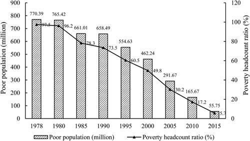
Since reform and opening up of the Chinese economy in the late 1970s, the government has initiated a series of poverty alleviation plans (Lü, 2015; Meng, 2013). For example, the Chinese government launched the 8-7 National Poverty Reduction Program in 1994, aiming to lift 80 million citizens out of poverty. In 2001, the Program for Poverty Alleviation and Rural Development was implemented to advance rural development. Over 1978 to 2015, the number of poor people in China reduced sharply from 770.39 million to 55.75 million (Figure 1). A total of 714.64 million people were out of poverty, accounting for more than 90% of the global reduction in the size of the population in poverty (Chen & Jin, 2017). Meanwhile, the country’s poverty headcount ratio (the proportion of the poorest in the total population) declined from 97.5% to 3.1% over the same period, with an average annual decrease of 11.48% (Figure 1). Specifically, the ratio has fallen sharply to an average of 14.7%, annually, since the year 2000.

Figure 1. National trends in China’s official poverty headcount, 1978–2015.

Source: The Central People’s Government (2018).

Despite these successes in poverty reduction, China’s development is regionally quite unbalanced, and hence the country continues to suffer severe relative poverty (Liu & Xu, 2016; Zhou et al., 2018). There are still 16.34 million poor people in the rural areas of western China, as of 2017, accounting for more than half of the country’s rural poor (National Bureau of Statistics of China, 2018). Additionally, the poverty headcount ratio in China’s ethnic areas remains above 10%, three times higher than that of the country as a whole (National Bureau of Statistics of China, 2018). As a result of the uneven development, China’s urban-rural income ratio reached 2.7 in 2017, much higher than the international level of 1.5 (Westmore, 2018). Therefore, the poverty problem in China still needs considerable attention.

2.2. Analytical framework of the Impact of Rural Financial Development on Poverty reduction

The literature on poverty traps argues that persistent poverty is driven by external constraints, such as credit market imperfections (Banerjee & Newman, 1991; Lü, 2015). Credit market failure arising from asymmetric information results in unequal access to credit and financial inefficiency (Galor & Zeira, 1993; Sehrawat & Giri, 2016). In this respect, financial institutions tend to allocate credit to those with whom they have established a relationship and who can provide sound collateral (Jalilian & Kirkpatrick, 2005). Rural financial development increases the probability for the lower-income class to obtain formal credit by addressing the causes of financial market failures, such as information and asymmetry (Jalilian & Kirkpatrick, 2005; Sehrawat & Giri, 2016).

Rural financial development can reduce poverty in at least two ways, the first, through access to agricultural credit, boosting agricultural productivity or technical efficiency (Agbodji & Johnson, 2019; Luan & Bauer, 2016; Nakano & Magezi, 2020). In developing nations, lack of capital hinders agricultural development and thus, rural finance plays an essential role in increasing investments in farming. Specifically, the availability of rural credit makes it possible for farmers to enhance the use of inputs such as pesticide and chemical fertilizer use, and animal feed, as well as increase land transfer (Luan & Bauer, 2016; Nakano & Magezi, 2020). Meanwhile, rural credit enables farmers to adopt advanced agricultural technologies, such as irrigation, improved seeds, and the use of information and communication technologies (ICT). In addition, access to rural credit helps protect smallholders from the uncertainties of nature (e.g., climate change, phytosanitary diseases, pests and animal diseases) (Agbodji & Johnson, 2019). These uses of agricultural credit may have positive effects on agricultural productivity, and in turn, on poverty.

Moreover, access to rural credit may increase farmers’ off-farm earnings, thereby diversifying their sources of income (Burgess & Pande, 2005; Luan & Bauer, 2016; Qian & Huang, 2016). First, rural credit enables the financing of township enterprises that create employment for the poor population (Qian & Huang, 2016). Second, subsidized rural loans may encourage farmers to engage in profitable off-farm activities and encourage them to venture into entrepreneurship (Luan & Bauer, 2016). Therefore, to some extent, rural financial development reduces poverty through off-farm employment in developing countries.

3. Materials and methods

3.1. Data sources

We use a panel dataset of 30 provinces (out of 31) in mainland China from 1997 to 2015. One province, the Tibet Autonomous Region, is excluded because of a significant lack of data. The research range begins in 1997 due to the availability of data. Our study sample covers 19 years of development in China. The long time span enables us to examine in depth the impact of rural financial development on poverty reduction in China.

In China, rural finance is composed of formal rural and informal rural finance, and our focus is on formal rural finance. Formal rural finance is licensed and regulated by China’s monetary authority, mainly Rural Credit Cooperatives (RCC), the Agricultural Bank of China, the Postal Savings Bank of China, and the Agricultural Development Bank of China. The data released by the Development Research Centre of the State Council (2018) reveal that the RCCs’ rural credit scale reached RMB 3.7 trillion in 2015, accounting for 68.52% of the national rural credit. Almost 800 million RCCs are distributed across grassroots townships, making it convenient for farmers to access financial services. Thus, the RCC is the main channel through which farmers can obtain formal financial services. Therefore, we use the rural credit scale from the China Financial Yearbook (1997–2015) in this study to investigate China’s rural financial development.

In addition, data on food consumption and gross family expenditure are obtained from the China Rural Statistical Yearbook (1997–2015). Data from the state-owned RCC are used to measure the scale of rural credit since the cooperative is the main channel for China’s farmers to obtain formal financial services. Data on urbanization, fiscal expenditure for agriculture development, mechanization, fixed asset investment, and gross agricultural output value are obtained from the China Statistical Yearbook (1997–2015).

3.2. Specification of the empirical model: spatial panel data models

Tobler’s First Law of Geography states that everything on a geographical surface is related to everything else, but near things are more related to each other than distant things (Tobler, 1970). Rural finance, as a factor of capital, can flow among the capital markets of neighbouring regions. In other words, rural financial development leads to interaction effects among regions. Therefore, the impact of rural financial development on poverty reduction may have spatial spillover effects. Conventional econometric methods may underestimate the effect of rural financial development by ignoring spatial correlation (Anselin et al., 1996).

The most commonly used spatial panel data models are the spatial lag model (SLM), the spatial error model (SEM), and the spatial Durbin model (SDM). The SLM model is appropriate for situations where there are endogenous interaction effects among the dependent variables. The SEM model fits into situations where there are interaction effects among the error terms. The SDM model is derived from a combination of the SLM model and the SEM model (LeSage & Fischer, 2008). In our study, the three spatial panel data models are respectively specified as follows: (1) $$\begin{array}{cc}{\text{POVERTY}}_{it}=\rho \sum _{j=1}^n{w}_{ij}P\mathit{OVERT}{Y}_{jt}+\alpha \mathit{FINANCIA}{L}_{\text{it}}+X_{it}\beta +{\tau }_i+{\epsilon }_{it}& \text{SLM}\end{array}$$(1) (2) $$\begin{array}{cc}{\text{POVERTY}}_{it}=\alpha \mathit{FINANCIA}{L}_{\text{it}}+X_{it}\beta +\lambda \sum _{j=1}^n{w}_{ij}{\phi }_{jt}+{\tau }_i+{\epsilon }_{it}& \text{SEM}\end{array}$$(2) (3) $$\begin{array}{cc}\mathit{POVERT}{Y}_{it}=\rho \sum _{j=1}^n{w}_{ij}P\mathit{OVERT}{Y}_{jt}+\alpha \mathit{FINANCIA}{L}_{\text{it}}+X_{it}\beta +\theta \sum _{j=1}^n{w}_{ij}F\mathit{INANCIA}{L}_{jt}+\sum _{j=1}^n{w}_{ij}{X}_{jt}\gamma +{\tau }_i+{\epsilon }_{it}& \text{SDM}\end{array}$$(3)

POVERTY_it is the poverty level in i^th province in t^th year. In terms of measuring poverty, most studies use the poverty headcount ratio to reflect the poverty level in a country or region (Imai et al., 2012; Perez-Moreno, 2011; Wossen et al., 2019). Nevertheless, data on the poverty headcount ratio at the provincial level is not available. Therefore, we follow previous studies (Bargain et al., 2014; Cherchye et al., 2012) and select the Engel index, a ratio of food consumption to gross family expenditure, as a measure of the poverty level.

FINANCIAL_it is the key explanatory variable and is measured by the ratio of rural credit scale to the gross agricultural output value. At the macro level, financial development is usually measured from the three dimensions of scale, structure and efficiency (Jiang et al., 2020; Zheng, 2017). In this study, we do not use the rural financial structure as a measurement of financial development because rural finance rarely refers to stock transactions in China. Following existing literature (Akhter & Daly, 2009; Beck et al., 2007; Edmans et al., 2016; Jeanneney & Kpodar, 2011), we select the other two indicators, rural financial scale and rural financial efficiency, as proxy for financial development. Specifically, the first indicator is used in the main models and the second is employed to conduct a relevant robustness check.

X_it is a vector of control variables. Specifically, our control variables include urbanization, which is the ratio of urban population to total population; fiscal expenditure for agriculture development, which is the ratio of fiscal expenditure for agriculture development to gross agricultural output value; mechanization, which is measured by the ratio of total agricultural machinery power in the countryside to the number of rural labourers; fixed asset investment, which is measured by the ratio of fixed asset investment in rural areas to gross agricultural output value; and average gross agricultural output value, which is the ratio of gross agricultural output value to the number of rural labourers. Table 1 presents the details of the variable settings. The parameters ρ and ɛ_it are the spatial autoregressive coefficient and random disturbance term, respectively; τ_i is province fixed effects. λ denotes the spatial autocorrelation coefficient of the error term φ; γ presents the matrix of the spatial autocorrelation coefficient; and w_ij is the element in an n × n spatial weight matrix W, where we assume w_ij equals the reciprocal of the difference of the geographical distance between region i and j if i is not equal to j, and is zero otherwise.

Table 1. Definitions, codes, and measurement methods of the variables. 

Name of variable	Definition of variable	Calculation
POVERTY	Poverty level	Food consumption / gross family expenditure
FINANCIAL	Rural financial development	Rural credit scale / gross agricultural output value
URBAN	Urbanization	Urban population / total population
FISCAL	Fiscal expenditure for agriculture development	Fiscal expenditure for agriculture development / gross agricultural output value
MECHANIZATION	Mechanization	Total agricultural machinery power in rural areas / number of rural labourers
FASSET	Fixed asset investment	Fixed asset investment in rural areas / gross agricultural output value
AAOUTPUT	Average agricultural output value	Gross agricultural output value / number of rural labourers
RELIEF	Rural social relief	Rural social relief / total fiscal expenditure
DISATER	Agricultural disaster area	Agricultural disaster area / total sowing area
HIGHWAY	Highway mileage	Highway mileage (10,000 km)

Source: Authors' definition.

Before using the spatial panel data models, we need to examine whether there is spatial dependence among regions. The most commonly used method to examine spatial dependence is Moran’s I, which is expressed as follows: (4) $$\mathit{Moran}`s I=\frac{\sum _{i=1}^n\sum _{j=1}^n{w}_{ij}(x_i-\overline{x})(x_j-\overline{x})}{S^2\sum _{i=1}^n\sum _{j=1}^n{\omega }_{ij}}$$(4) where x_i, $\overline{x}$ x, and S² represent the observed value, sample mean, and sample variance, respectively. Moran’s I ranges from −1 to 1. If its value is less than 0, there is negative autocorrelation among regions; if its value is greater than 0, there is positive autocorrelation between units. The closer to 1 the Moran’s I value is, the greater the difference between units, and the higher the degree of aggregation. If it is equal to 0, there is no correlation between the units.

After examining spatial dependence, the next step is to check which spatial panel data model is the best fit for our data. First, if the first null hypothesis H₀: γ = 0 is never rejected by the Wald test, the SLM model is more appropriate than the SDM model, that is, the SDM model can be pre-digested to the SLM model. Second, the SEM model better fits our data if the second null hypothesis H₀: γ + ρβ = 0 is never rejected by the LR test, meaning the SDM model can be simplified to the SEM model. Finally, when both null hypotheses are rejected, we argue that the SDM model best describes our data.

3.3. Estimation for direct, indirect, and total effects

The coefficients of independent variables estimated by the maximum likelihood (ML) model cannot describe the marginal effect in the spatial panel model, including the spatial lags of explanatory and dependent variables. Thus, it is necessary to further calculate the direct, indirect, and total effects of the explanatory variables on the dependent variable. In this study, if the rural financial development level in a particular province were to change, it would have an impact on the poverty level of the province as well as of the contiguous provinces. The direct and indirect effects, or spatial spillover, comprise the total effect.

To elucidate the computation of the direct, indirect, and total effects based on the SDM model, we form: (5) $$y={(I_n-\rho W)}^{-1}(\mathrm{X}\alpha +\text{WX}\gamma )+{(I_n-\rho W)}^{-1}\epsilon$$(5) where I_n denotes an identity matrix and the other parameters are the same as stated above. If X includes k explanatory variables, we can further derive: (6) $$y={\sum }_{r=1}^k{S}_r(W)x_r+{(I_n-\rho W)}^{-1}WX\gamma +{(I_n-\rho W)}^{-1}\epsilon$$(6) where x_r represents the r^th explanatory variable and S_r(W) is equal to α_r(I-λW)⁻¹. We transfer Equation (6)(6) $$y={\sum }_{r=1}^k{S}_r(W)x_r+{(I_n-\rho W)}^{-1}WX\gamma +{(I_n-\rho W)}^{-1}\epsilon$$(6) to a matrix form: (7) $$\left(\begin{array}{c}{y}_1\\ y_2\\ ⋮\\ y_n\end{array}\right)=\left(\begin{array}{cccc}{S}_r{(W)}_{11}& S_r{(W)}_{12}& \cdots & S_r{(W)}_{1n}\\ S_r{(W)}_{21}& S_r{(W)}_{22}& \cdots & S_r{(W)}_{2n}\\ ⋮& ⋮& & ⋮\\ S_r{(W)}_{n1}& S_r{(W)}_{n2}& \cdots & S_r{(W)}_{nn}\end{array}\right)\left(\begin{array}{c}{x}_{1r}\\ x_{2r}\\ ⋮\\ x_{nr}\end{array}\right)+{\left(I_n-\rho W\right)}^{-1}WX\gamma +{\left(I_n-\rho W\right)}^{-1}\epsilon$$(7)

The average direct, total, and indirect effects can be calculated as follows, respectively: (8) $$\overline{M}{(r)}_{\mathit{direct}}=n^{-1}t\mathit{race}[S_r(W)]$$(8) (9) $$\overline{M}{(r)}_{\mathit{total}}=n^{-1}{l}_n^{\prime }{S}_r(W)l_n$$(9) (10) $$\overline{M}{(r)}_{\mathit{indirect}}=\overline{M}{(r)}_{\mathit{total}}-\overline{M}{(r)}_{\mathit{direct}}$$(10)

4. Summary statistics and empirical results

4.1. Summary statistics

Table 2 presents the summary statistics of the variables used in the model. All variables have 570 observation values. Over 1997 to 2015, the average poverty level (the Engel index) in China was 0.440, with a minimum of 0.273 (Shaanxi in 2013) and a maximum of 0.696 (Guizhou in 1997). On average, rural financial development was 0.686, and its minimum and maximum levels were 0.027 (Jiangsu in 2015) and 5.51 (Shanghai in 2015), respectively. The average urbanization level was 0.414, with a minimum of 0.110 (Guangxi in 2005) and a maximum of 0.901 (Shanghai in 2009). The average fiscal expenditure for agriculture development was only 0.089 and the maximum is 0.236. The average values of mechanization level, fixed asset investment, and agricultural output are 1.031, 0.110, and 0.798, respectively. Over 1997 to 2015, the average rural social relief was 0.010 with minimum and maximum levels of 0.0001 and 0.212, respectively. The average agricultural disaster area and highway mileage were 0.270 and 9.04, respectively.

Table 2. Summary statistics of the variables.

Code	Obs	Mean	Std. Dev	Min	Max
POVERTY	570	0.440	0.086	0.273	0.696
FINANCIAL	570	0.686	0.831	0.027	5.510
URBAN	570	0.414	0.189	0.110	0.901
FISCAL	570	0.089	0.032	0.021	0.236
MECHANIZATION	570	1.031	0.675	0.151	3.817
FASSET	570	0.110	0.050	0.001	0.302
AAOUTPUT	570	0.798	0.641	0.127	1.415
RELIEF	570	0.010	0.020	0.0001	0.212
DISATER	570	0.270	0.164	0.000	0.936
HIGHWAY	570	9.040	6.684	0.396	31.558

Source: Authors' calculation.

4.2. Spatial autocorrelation test

Table 3 presents the results of the spatial autocorrelation test of the poverty level. We estimate the Moran’s I value of the poverty level for each year from 1997 to 2015. From Table 3, we can see that the Moran’s I value changes at approximately 0.5 and is consistently significant at 1% level, suggesting that the poverty level has spatial autocorrelation among neighbouring provinces. Therefore, spatial panel data models better fit our data than conventional panel models do.

Table 3. Spatial autocorrelation test of the poverty level from 1997 to 2015.

Year	Moran’s I	Year	Moran’s I
1997	0.417***	2007	0.602***
1998	0.470***	2008	0.610***
1999	0.597***	2009	0.555***
2000	0.621***	2010	0.681***
2001	0.603***	2011	0.558***
2002	0.591***	2012	0.546***
2003	0.606***	2013	0.564***
2004	0.579***	2014	0.549***
2005	0.591***	2015	0.516***
2006	0.683***	—	—

Note: ***, **, and *denote significance at the 1%, 5%, and 10% level, respectively.

Source: Authors' calculation.

4.3. Panel unit root tests and cointegration tests

Data on all variables are required to be stationary before constructing a panel model; otherwise, the regression results will be spurious. Therefore, panel unit root tests are used to examine whether our variables are stationary. The most common unit root tests in panel data include the Levin-Lin-Chu (LLC) test, the Harris–Tzavalis (HT) test, the Breitung test, and the Im-Pesaran-Shin (IPS) test (Cai et al., 2018). The first three approaches ignore the heterogeneity among provinces when compared with the IPS test (Im et al., 2003). Therefore, the IPS test is commonly used to test for the stationarity in the panel data. To improve the robustness of the unit root test, we also report the results of the HT test in Table 4. As shown in Table 4, the results of the HT test are quite similar to those of the IPS test: excluding URBAN, MECHANIZATION, and AAOUTPUT, the variables are significantly stationary. Nevertheless, URBAN, MECHANIZATION, AAOUTPUT, DISATER, RELIEF, and HIGHWAY reach significant stationarity after the first difference, that is, the three variables are integrated to the order one, implying the necessity to explore whether there is a long-term equilibrium between unit root variables and dependent variables.

Table 4. Panel unit root test.

Variables	IPS (Level)	IPS (First difference)	HT (Level)	HT (First difference)
POVERTY	−5.282***		0.504***
FINANCIAL	−2.341***		0.574**
URBAN	−0.914	−7.747***	0.755	0.427***
FISCAL	−7.199***		0.110***
MECHANIZATION	2.580	−8.738***	0.794	0.330***
FASSET	−3.188***	−6.433***	0.725***
AAOUTPUT	2.262	−7.804***	0.909	0.413***
RELIEF	16.502	−6.739***	1.366	0.497***
DISATER	−11.129***		−0.137***
HIGHWAY	4.327	−10.749***	0.607	0.080***

Note: ***, **, and * denote significance at the 1%, 5%, and 10% level, respectively.

Source: Authors' calculation.

Then, we perform panel cointegration tests using the Pedroni test and the Kao test. From Table 5, we can see that most of the Pedroni test, except for the panel rho-statistic of (0,0) and the panel PP-statistic of (1,0), demonstrate the cointegration relationship between unit root variables and dependent variables. Similarly, the Kao test rejects the null hypothesis of no cointegration. Accordingly, we can construct the spatial econometric model directly.

Table 5. Panel cointegration test.

Pedroni test	Category	(0,0)	(1,0)	(1,1)
	Panel v-Statistic	−4.512***	−1.770**	−1.830**
	Panel rho-Statistic	2.258**	1.024	1.857**
	Panel PP-Statistic	−1.205	−3.523***	−4.734***
	Panel ADF-Statistic	−2.168**	−4.393***	−5.921***
	Group rho-Statistic	4.014***	2.663***	3.894***
	Group PP-Statistic	−1.492*	−3.758***	−3.601***
	Group ADF-Statistic	−2.978***	−4.736***	−5.182***
Kao test	ADF-statistic	—	−5.6781***	—

Note: Both the Pedroni test and the Kao test hypothesize that there is no cointegration relationship. In the Pedroni test, the first four and last three rows report the results within dimensions and between dimensions, respectively. The three columns to the right exhibit the results accounting for neither individual fixed effect nor linear time trend (column (0,0)), for individual fixed effect only (column (0,1)), and for both separately (column (1,1)).

***, **, and *denote significance at the 1%, 5%, and 10% level, respectively.

Source: Authors' calculation.

4.4. Regression results of rural financial development on poverty level

In contrast with the spatial econometric model, we first estimate a conventional fixed effect panel model without spatial interaction effects. The results are shown in column (1) of Table 6. Our study demonstrates that the coefficient of FINANCIAL is significantly negative, suggesting that rural financial development would reduce poverty. The preliminary finding is consistent with the existing literature (Agbola et al., 2017; Imai et al., 2010).

Table 6. Regression results of rural financial development on poverty level.

Variables	(1) FE	(2) SDM	(3) Direct	(4) Indirect	(5) Total
FINANCIAL	−0.094**	−0.048**	−0.063***	−0.139**	−0.202**
	(0.039)	(0.020)	(0.022)	(0.068)	(0.079)
URBAN	−0.026	−0.046*	−0.005	0.380***	0.375***
	(0.042)	(0.023)	(0.023)	(0.115)	(0.127)
FISCAL	0.088	−0.179**	−0.070	0.926**	0.855**
	(0.120)	(0.078)	(0.090)	(0.379)	(0.423)
MECHANIZATION	−0.017	−0.011*	−0.016**	−0.048**	−0.064**
	(0.017)	(0.006)	(0.008)	(0.024)	(0.029)
FASSET	−0.378**	−0.417***	−0.488***	−0.560***	−1.048***
	(0.147)	(0.038)	(0.053)	(0.140)	(0.179)
AAOUTPUT	−0.039***	−0.031***	−0.036***	−0.048**	−0.084***
	(0.010)	(0.006)	(0.006)	(0.019)	(0.021)
RELIEF	−0.547***	−0.353***	−0.427***	−0.651**	−1.079***
	(0.099)	(0.084)	(0.077)	(0.293)	(0.303)
DISATER	0.022	0.012	0.007	−0.031	−0.025
	(0.014)	(0.010)	(0.009)	(0.030)	(0.033)
HIGHWAY	−0.005***	−0.003***	−0.004***	−0.007***	−0.011***
	(0.001)	(0.001)	(0.000)	(0.002)	(0.002)
Constant	0.639***
	(0.041)
ρ		5900.964***
		(422.093)
Wald test		19.01***
LR test		27.33***
R-squared	0.478	0.571
Observations	570	570

Note: The standard error is in parentheses.

***, **, and * denote significance at the 1%, 5%, and 10% level, respectively. The spatial lag explanatory variables of the SDM model are reported in Appendix Table A1, column (1).

Source: Authors' calculation.

The Wald test and the LR test suggest that the SDM model is preferred over the SLM model and the SEM model. Column (2) in Table 6 shows the results from the SDM model with a fixed effect. It is noteworthy that FINANCIAL has a significantly negative impact on the poverty level when we take spatial interaction effects into consideration. However, we should note that the coefficients of the SDM model do not reflect the partial effects of the explanatory variables. Hence, based on Equations (5)(5) $$y={(I_n-\rho W)}^{-1}(\mathrm{X}\alpha +\text{WX}\gamma )+{(I_n-\rho W)}^{-1}\epsilon$$(5) to (10)(10) $$\overline{M}{(r)}_{\mathit{indirect}}=\overline{M}{(r)}_{\mathit{total}}-\overline{M}{(r)}_{\mathit{direct}}$$(10) , we estimate the direct, indirect, and total effects of the explanatory variables (see columns (3) to (5) in Table 6). It is surprising that the direct effects of independent variables in column (3) differ from their coefficient estimates in column (2) of Table 6. For example, the coefficient estimate of FINANCIAL is −0.048 while the direct effect is −0.063. This difference may be due to the feedback effect of FINANCIAL attributed to the endogenous interaction effect (Wy). In other words, the feedback effect of FINANCIAL refers to how FINANCIAL in a certain province affects contiguous provinces and then rebounds to the original province.

Our interest lies in the indirect effects. In terms of our key explanatory variable, FINANCIAL, the spatial spillover effect amounts to −0.139, accounting for 68.81% (0.139/0.202) of the total effect. The result suggests that rural financial development in a region significantly alleviates poverty in a neighbouring region. Such spillover effects of financial development on poverty alleviation are not noted in the literature (Agbola et al., 2017; Berhane & Gardebroek, 2011; Imai et al., 2010), which typically assumes that financial development is independent between regions. One interpretation of the indirect effect is that rural finance, as a factor of capital, flows among the capital markets of proximate regions (Jin et al., 2017). Another reason could be the diffusion effects of local rural financial policies. Specifically, if rural financial development contributes to poverty reduction in a certain region, the model is likely to be replicated by the neighbouring regions, contributing to policy implications for poverty alleviation in these regions (Seven & Coskun, 2016).

Furthermore, the total effect coefficient of FINANCIAL is −0.202, which is larger than that of conventional fixed effects methods (-0.094), suggesting that the conventional fixed-effect model underestimates the effect of rural financial development when ignoring the spatial spillover effect. Similarly, existing studies (Goel & Saunoris, 2020; You & Lv, 2018) also confirm the underestimation from the conventional panel model due to the failure of spatial correlation. For example, You and Lv (2018) employ the SDM technique to investigate the impact of economic globalization on CO₂ emissions and conclude that the conventional panel model underestimates the effect by approximately 27 per cent.

4.5. Robustness check

Given that the causal relationship between poverty level and rural financial development may be bidirectional, we conduct a robustness check using an instrumental variable to address the endogeneity problem. We select the one-period lag of FINANCIAL as an instrumental variable according to the Akaike Information Criterion (Zhao et al., 2018). First, our instrumental variable satisfies the first condition of instrumental variables, as the one-period lag of FINANCIAL is a predetermined variable that meets the exogenous principle. Second, the one-period lag of FINANCIAL is highly relevant to FINANCIAL of the current period, satisfying the second condition that the instrumental variable should be correlated to the endogenous variable. Column (1) of Table 7 shows that both the Anderson Canon LM statistic and the Cragg-Donald Wald F statistic are significant at the 1% level. Hence, the one-period lag of FINANCIAL is an identifiable and valid instrument variable for FINANCIAL. The two-stage least square (2SLS) result in column (1) of Table 7 implies that FINANCIAL still has a significantly negative effect on the poverty level. In addition, the 2SLS still underestimates the effect of rural financial development on poverty reduction compared with the total effect of rural financial development in column (5) of Table 6. It is noteworthy that the significance and sign for the coefficients of control variables in the 2SLS model (see column (1) of Table 7) are similar to those in the SDM model in column (2) of Table 6. Thus, based on a comparison between SDM and 2SLS, we conclude that the estimation of SDM is relatively robust.

Table 7. Results of robustness check.

Variables	(1) 2SLS	Using rural financial efficiency as a proxy variable of FINANCIAL
		(2) SDM	(3) Direct	(4) Indirect	(5) Total
FINANCIAL	−0.078**	−0.019***	−0.021***	−0.017**	−0.038***
	(0.031)	(0.003)	(0.004)	(0.007)	(0.009)
URBAN	−0.013	−0.058***	−0.008	0.470***	0.462***
	(0.025)	(0.023)	(0.022)	(0.114)	(0.125)
FISCAL	−0.023	−0.160**	−0.056	0.903**	0.847**
	(0.091)	(0.076)	(0.087)	(0.362)	(0.402)
MECHANIZATION	−0.013*	−0.019***	−0.028***	−0.081***	−0.109***
	(0.007)	(0.006)	(0.008)	(0.025)	(0.031)
FASSET	−0.373***	−0.397***	−0.447***	−0.381***	−0.828***
	(0.051)	(0.038)	(0.052)	(0.130)	(0.168)
AAOUTPUT	−0.039***	−0.029***	−0.032***	−0.021	−0.053**
	(0.006)	(0.005)	(0.006)	(0.021)	(0.023)
RELIEF	−0.554***	−0.326***	−0.396***	−0.624**	−1.019***
	(0.085)	(0.083)	(0.078)	(0.273)	(0.282)
DISATER	0.016	0.009	0.002	−0.050	−0.048
	(0.012)	(0.010)	(0.009)	(0.031)	(0.033)
HIGHWAY	−0.005***	−0.003***	−0.004***	−0.007***	−0.010***
	(0.001)	(0.001)	(0.000)	(0.002)	(0.002)
Constant	0.624***
	(0.026)
Anderson Canon LM	300.811***
Cragg-Donald Wald F	720.434
ρ		5797.702***
		(428.966)
R-squared	0.420	0.077
Observations	540	570

Note: The standard error is in parentheses.

***, **, and *denote significance at the 1%, 5%, and 10% level, respectively. The spatial lag explanatory variables of the SDM model are reported in Appendix Table A1, column (2).

Source: Authors' calculation.

Another robustness check is employed by substituting a proxy variable for FINANCIAL. Our proxy variable, rural financial efficiency, is defined by the ratio of rural credit scale to rural saving scale. The empirical result with the proxy variable indicates that FINANCIAL still contributes to poverty reduction (see column (2) in Table 7). Furthermore, the indirect effect (spatial spillover effect) of FINANCIAL using the proxy variable amounts to −0.017, again confirming the spatial spillover effect of rural financial development. Despite the numerous checks, our finding that rural financial development promotes poverty reduction and exhibits spatial spillover effect is always robust.

4.6. Regression results of rural financial development on urban-rural inequality

Our analysis shows that rural financial development promotes poverty reduction and has spatial spillover effects. To determine whether rural financial development narrows the urban-rural income gap, the ratio of China’s urban-rural residential income (per capita disposable income of urban residents/per capita disposable income of rural residents) is selected as the explained variable based on Equation (1) to (3)(3) $$\begin{array}{cc}\mathit{POVERT}{Y}_{it}=\rho \sum _{j=1}^n{w}_{ij}P\mathit{OVERT}{Y}_{jt}+\alpha \mathit{FINANCIA}{L}_{\text{it}}+X_{it}\beta +\theta \sum _{j=1}^n{w}_{ij}F\mathit{INANCIA}{L}_{jt}+\sum _{j=1}^n{w}_{ij}{X}_{jt}\gamma +{\tau }_i+{\epsilon }_{it}& \text{SDM}\end{array}$$(3) . Using the SDM model with fixed effects, column (1) to (3) in Table 8 shows that rural financial development significantly widens the gap between urban and rural areas, and has a significant spillover effect on the urban-rural income gap (see column (2) in Table 8). The finding is nearly in line with Ge et al. (2015), though they do not take spatial correlation into account. However, Xiao et al. (2020) conclude that the urban-rural income gap can be narrowed through rural inclusive finance.

Table 8. Regression results of rural financial development on urban-rural income inequality.

Variables	Urban-rural income inequality			Per capita income of urban residents (10,000 yuan)			Per capita income of rural residents (10,000 yuan)
	(1) Direct	(2) Indirect	(3) Total	(4) Direct	(5) Indirect	(6) Total	(7) Direct	(8) Indirect	(9) Total
FINANCIAL	0.080***	0.156***	0.236***	0.049***	0.011***	0.059***	0.014***	0.002	0.016***
	(0.027)	(0.044)	(0.059)	(0.003)	(0.003)	(0.005)	(0.001)	(0.002)	(0.002)
URBAN	−0.169	−1.919***	−2.088**	0.182***	−0.135**	0.047	0.044***	−0.022	0.022
	(0.164)	(0.739)	(0.811)	(0.018)	(0.055)	(0.054)	(0.006)	(0.026)	(0.027)
FISCAL	−1.184*	−2.882	−4.066*	0.098	−0.949***	−0.851***	0.000	−0.310***	−0.309***
	(0.643)	(2.210)	(2.433)	(0.077)	(0.178)	(0.182)	(0.028)	(0.086)	(0.093)
MECHANIZATION	0.236***	1.046***	1.282***	−0.017***	0.054***	0.037***	−0.012***	−0.008	−0.021***
	(0.057)	(0.176)	(0.209)	(0.006)	(0.011)	(0.014)	(0.002)	(0.005)	(0.007)
FASSET	−0.595	−1.300*	−1.895*	−0.025	−0.131**	−0.156*	0.015	0.039	0.055
	(0.380)	(0.733)	(1.009)	(0.043)	(0.054)	(0.080)	(0.016)	(0.028)	(0.040)
AAOUTPUT	−0.149***	−0.534***	−0.683***	0.082***	0.028**	0.110***	0.042***	0.036***	0.078***
	(0.042)	(0.137)	(0.153)	(0.005)	(0.011)	(0.011)	(0.002)	(0.005)	(0.006)
RELIEF	−3.044***	−6.495***	−9.539***	0.047	0.760***	0.807***	0.048*	0.505***	0.553***
	(0.608)	(1.814)	(1.848)	(0.080)	(0.145)	(0.126)	(0.028)	(0.068)	(0.067)
DISATER	0.207***	0.105	0.311	0.017**	−0.023	−0.006	0.002	0.001	0.003
	(0.067)	(0.202)	(0.211)	(0.008)	(0.016)	(0.016)	(0.003)	(0.008)	(0.008)
HIGHWAY	0.002	0.044***	0.046***	0.002***	0.003***	0.004***	0.001***	−0.000	0.000
	(0.004)	(0.010)	(0.011)	(0.000)	(0.001)	(0.001)	(0.000)	(0.000)	(0.000)
ρ	5102***			1643***			4294***
	526.112			483.322			489.310
R-squared	0.023			0.741			0.710
Observations	570			570			570

Note: The standard error is in parentheses.

***, **, and *denote significance at the 1%, 5%, and 10% levels, respectively. The spatial lag explanatory variables of the SDM model are reported in Appendix Table A1, column (3) to (5). Yuan is Chinese currency unit, 1 Yuan ≈0.15 US dollar in 2020.

Source: Authors' calculation.

We also estimate the effects of rural financial development on the per capita income of urban residents and of rural residents separately. Our results indicate that rural financial development significantly increases the per capita income of rural residents, with a direct effect of 0.014 and a total effect of 0.016 (see column (7) and (9) in Table 8). Additionally, rural financial development significantly improves the per capita income of urban residents (see column (4) to (6) in Table 8), and its total effect is higher than that of rural financial development on per capita income of rural residents.

One probable explanation of why rural financial development polarizes urban-rural income is the urban-rural financial exclusion (Ge et al., 2015). Specifically, the urban elite enjoys favourable economic conditions. This means that the Rural Credit Cooperative is more likely to provide them with rural credit for investment in agriculture. As a consequence, some smallholders are excluded from the rural financial market while the urban elite benefits more from rural credit programmes. Another reason is that agricultural enterprises financed by agricultural credit tend to expand the production scale and adopt superior technology, which improves returns to scale and boosts the township economy. Meanwhile, agricultural enterprises also create more employment opportunities for urban residents. Ultimately, rural financial development may indirectly grow urban residents’ income, but may not exert considerable influence on rural smallholders (Alatas et al., 2013; Platteau et al., 2014).

5. Conclusions and policy implications

Despite substantial efforts to fight poverty over the past four decades, the Chinese government goal of lifting the entire rural population out of poverty by 2020 remains a significant challenge. Financial development is an important way to alleviate poverty and has become an important research subject. Using the panel data of 30 provinces in China from 1997 to 2015, we employed the spatial Durbin model to re-examine the effect of rural financial development on poverty reduction. Our findings are as follows. First, rural financial development helps reduce poverty in rural China. Second, rural financial development has a positive spatial spillover effect on alleviating poverty for neighbouring regions. Third, rural financial development also widens the urban-rural inequality gap, proving the existence of financial exclusion in rural China. Finally, we find that a conventional panel model may underestimate the effect of rural financial development because it ignores the spatial spillover effect.

The findings of this research lead to three significant policy implications. Since the late 1970s, the Chinese government has implemented a series of poverty alleviation measures including living aid, non-agricultural employment, and field training (Liu et al., 2020). In the future, the government and enterprises should pay more attention to developing rural finance. We recommend that, first, modern credit platforms for rural areas be established to improve agricultural productivity or technical efficiency and encourage off-farm activities. Second, the existence of spatial spillover effects of rural financial development indicates that rural credit policies in surrounding areas are not completely independent, suggesting demonstration effects of rural credit policies. Thus, it is essential for the government to foster regional integration in rural financial development. Finally, despite subsidized loans for rural areas, the phenomenon of the elite capturing much of the rural credit market may result in urban-rural income inequality (Alatas et al., 2013; Platteau et al., 2014). Consequently, policymakers should design targeted credit strategies and strengthen oversight of the rural finance market to benefit the poorest.

Disclosure statement

No potential conflict of interest was reported by the authors.

Additional information

Funding

This research was supported by National Natural Science Foundation of China (71661147002, 71973011) and the Ministry of Science and Technology of China (2016YFD0201301)

Appendix A

Table A1. Estimates of spatial lag explanatory variables of SDM model.

Variables	(1) SDM	(2) SDM	(3) SDM	(4) SDM	(5) SDM
W*FINANCIAL	−707.974	−15.328	1049.200***	72.384	−34.987**
	(496.548)	(44.025)	(341.123)	(46.046)	(16.469)
W*URBAN	2937.943***	3752.501***	−17437.694***	−2245.036***	−441.003*
	(713.589)	(718.927)	(5527.041)	(683.807)	(242.940)
W*FISCAL	7863.626***	7766.501***	−20333.741	−13312.046***	−3215.234***
	(2450.840)	(2419.899)	(18230.862)	(2255.035)	(800.057)
W*MECHANIZATION	−263.453	−474.208***	8656.073***	800.661***	−30.583
	(174.317)	(166.884)	(1297.776)	(167.375)	(60.764)
W*FASSET	−1588.616*	−538.929	−9878.592	−1866.464**	318.987
	(823.814)	(814.888)	(6422.644)	(781.079)	(277.492)
W*AAOUTPUT	−167.675	9.439	−4224.951***	251.442	205.776***
	(142.997)	(144.409)	(1119.691)	(159.163)	(68.833)
W*RELIEF	−2661.014	−2805.910	−45910.248***	10448.813***	5079.205***
	(2088.708)	(2031.450)	(15936.823)	(2018.060)	(765.488)
W*DISATER	−313.635	−447.925*	−336.407	−381.631	−3.438
	(245.230)	(254.798)	(1973.367)	(244.204)	(86.742)
W*HIGHWAY	−34.338**	−33.649***	397.252***	32.847**	−4.129
	(13.687)	(13.035)	(103.323)	(13.226)	(4.392)

Note: The standard error is in parentheses.

***, **, and * denote significance at the 1%, 5%, and 10% level, respectively.

Source: Authors' calculation.

References

- Agbodji, A., & Johnson, A. (2019). Agricultural credit and its impact on the productivity of certain cereals in Togo. Emerging Markets Finance and Trade, 2019(10), 1–17. https://doi.org/https://doi.org/10.1080/1540496X.2019.1602038
- Agbola, F. W., Acupan, A., & Mahmood, A. (2017). Does microfinance reduce poverty? New evidence from northeastern Mindanao, the Philippines. Journal of Rural Studies, 50, 159–171. https://doi.org/https://doi.org/10.1016/j.jrurstud.2016.11.005
- Akhter, S., & Daly, K. J. (2009). Finance and poverty: Evidence from fixed effect vector decomposition. Emerging Markets Review, 10(3), 191–206. https://doi.org/https://doi.org/10.1016/j.ememar.2009.02.005
- Alatas, V., Banerjee, A., Hanna, R., Olken, B. A., Purnamasari, R., & Wai-Poi, M. (2013). Does elite capture matter? Local elites and targeted welfare programs in Indonesia. NBER Working Paper No. w18798, https://doi.org/https://doi.org/10.1257/pandp.20191047
- Anselin, L., Bera, A. K., Florax, R., & Yoon, M. J. (1996). Simple diagnostic tests for spatial dependence. Regional Science and Urban Economics, 26(1), 77–104. https://doi.org/https://doi.org/10.1016/0166-0462(95)02111-6
- Banerjee, A., & Newman, A. (1991). Risk-bearing and the theory of income distribution. The Review of Economic Studies, 58(2), 211–235. https://doi.org/https://doi.org/10.2307/2297965
- Bargain, O., Donni, O., & Kwenda, P. (2014). Intrahousehold distribution and poverty: Evidence from CÔte d’Ivoire. Journal of Development Economics, 107, 262–276. https://doi.org/https://doi.org/10.1016/j.jdeveco.2013.12.008
- Beck, T., Asli, D., & Levine, R. (2007). Finance, inequality and the poor. Journal of Economic Growth, 12(1), 27–49. https://doi.org/https://doi.org/10.1007/s10887-007-9010-6
- Berhane, G., & Gardebroek, C. (2011). Does microfinance reduce rural poverty? Evidence based on household panel data from northern Ethiopia. American Journal of Agricultural Economics, 93(1), 43–55. https://doi.org/https://doi.org/10.1093/ajae/aaq126
- Burgess, R., & Pande, R. (2005). Do rural banks matter? Evidence from the Indian social banking experiment. American Economic Review, 95(3), 780–795. https://doi.org/https://doi.org/10.1257/0002828054201242
- Cai, J., Zheng, Z., Hu, R., Pray, C. E., & Shao, Q. (2018). Has international aid promoted economic growth in Africa? African Development Review, 30(3), 239–251. https://doi.org/https://doi.org/10.1111/1467-8268.12333
- Carrer, M., Maia, A. G., Vinholis, M., & de Souza Filho, H. M. (2020). Assessing the effectiveness of rural credit policy on the adoption of Integrated Crop-Livestock Systems in Brazil. Land Use Policy, 92, 104468. https://doi.org/https://doi.org/10.1016/j.landusepol.2020.104468
- Chen, Z., & Jin, M. (2017). Financial inclusion in China: Use of credit. Journal of Family and Economic Issues, 38(4), 528–540. https://doi.org/https://doi.org/10.1007/s10834-017-9531-x
- Cherchye, L., De Rock, B., & Vermeulen, F. (2012). Economic well-being and poverty among the elderly: An analysis based on a collective consumption model. European Economic Review, 56(6), 985–1000. https://doi.org/https://doi.org/10.1016/j.euroecorev.2012.05.006
- Development Research Center of the State Council. (2018). Overview of rural financial development in China. http://www.drc.gov.cn/.sannong/543995.html
- Edmans, A., Heinle, M., & Huang, C. (2016). The real costs of financial efficiency when some information is soft. Review of Finance, 20(6), 2151–2182. https://doi.org/https://doi.org/10.1093/rof/rfw030
- Galor, O., & Zeira, J. (1993). Income distribution and macroeconomics. The Review of Economic Studies, 60 (1), 35–52. doi: 0.2307/2297811 https://doi.org/https://doi.org/10.2307/2297811
- Ge, L., Tao, X., & Wang, H. (2015). Local finance, urbanization and urban-rural income gap. China Population, Resources and Environment, 25(09), 93–99. https://doi.org/https://doi.org/10.3969/j.issn.1002-2104.2015.09.012
- Goel, R. K., & Saunoris, J. W. (2020). Spatial spillovers of pollution onto the underground sector. Energy Policy, 144, 111688. https://doi.org/https://doi.org/10.1016/j.enpol.2020.111688
- Guo, P., & Jia, X. (2009). The structure and reform of rural finance in China. China Agricultural Economic Review, 1(2), 212–226. https://doi.org/https://doi.org/10.1108/17561370910927444
- Hermes, N. (2014). Does microfinance affect income inequality? Applied Economics, 46(9), 1021–1034. https://doi.org/https://doi.org/10.1080/00036846.2013.864039
- Hussain, A., & Thapa, G. B. (2012). Smallholders’ access to agricultural credit in Pakistan. Food Security, 4(1), 73–85. https://doi.org/https://doi.org/10.1007/s12571-012-0167-2
- Im, K. S., Pesaran, M. H., & Shin, Y. (2003). Testing for unit roots in heterogeneous panels. Journal of Econometrics, 115(1), 53–74. https://doi.org/https://doi.org/10.1016/S0304-4076(03)00092-7
- Imai, K. S., Arun, T., & Annim, S. K. (2010). Microfinance and household poverty reduction: New evidence from India. World Development, 38(12), 1760–1774. https://doi.org/https://doi.org/10.1016/j.worlddev.2010.04.006
- Imai, K. S., Gaiha, R., Thapa, G., & Annim, S. K. (2012). Microfinance and poverty—A macro perspective. World Development, 40(8), 1675–1689. https://doi.org/https://doi.org/10.1016/j.worlddev.2012.04.013
- Jalilian, H., & Kirkpatrick, C. (2005). Does financial development contribute to poverty reduction? Journal of Development Studies, 41(4), 636–656. https://doi.org/https://doi.org/10.1080/00220380500092754
- Jeanneney, S. G., & Kpodar, K. (2011). Financial development and poverty reduction: Can there be a benefit without a cost? Journal of Development Studies, 47(1), 143–163. https://doi.org/https://doi.org/10.1080/00220388.2010.506918
- Jiang, M., Luo, S., & Zhou, G. (2020). Financial development, OFDI spillovers and upgrading of industrial structure. Technological Forecasting and Social Change, 155, 119974. https://doi.org/https://doi.org/10.1016/j.techfore.2020.119974
- Jin, S., Guo, H., Delgado, M., & Wang, H. (2017). Benefit or damage? The productivity effects of FDI in the Chinese food industry. Food Policy, 68, 1–9. https://doi.org/https://doi.org/10.1016/j.foodpol.2016.12.005
- Khandker, S. R., & Koolwal, G. B. (2010). How infrastructure and financial institutions affect rural income and poverty: Evidence from Bangladesh. The Journal of Development Studies, 46(6), 1109–1137. https://doi.org/https://doi.org/10.1080/00220380903108330
- LeSage, J. P., & Fischer, M. M. (2008). Spatial growth regressions: Model specification, estimation and interpretation. Spatial Economic Analysis, 3(3), 275–304. https://doi.org/https://doi.org/10.1080/17421770802353758
- Liu, M., Feng, X., Wang, S., & Qiu, H. (2020). China's poverty alleviation over the last 40 years: Successes and challenges. Australian Journal of Agricultural and Resource Economics, 64(1), 209–228. https://doi.org/https://doi.org/10.1111/1467-8489.12353
- Liu, Y., & Xu, Y. (2016). A geographic identification of multidimensional poverty in rural China under the framework of sustainable livelihoods analysis. Applied Geography, 73, 62–76. https://doi.org/https://doi.org/10.1016/j.apgeog.2016.06.004
- Lü, X. (2015). Intergovernmental transfers and local education provision–Evaluating China’s 8-7 National Plan for poverty reduction. China Economic Review, 33, 200–211. https://doi.org/https://doi.org/10.1016/j.chieco.2015.02.001
- Luan, D. X., & Bauer, S. (2016). Does credit access affect household income homogeneously across different groups of credit recipients? Evidence from rural Vietnam. Journal of Rural Studies, 47, 186–203. https://doi.org/https://doi.org/10.1016/j.jrurstud.2016.08.001
- Mendola, M. (2007). Agricultural technology adoption and poverty reduction: A propensity-score matching analysis for rural Bangladesh. Food Policy, 32(3), 372–393. https://doi.org/https://doi.org/10.1016/j.foodpol.2006.07.003
- Meng, L. (2013). Evaluating China’s poverty alleviation program: A regression discontinuity approach. Journal of Public Economics, 101(1), 1–11. https://doi.org/https://doi.org/10.1016/j.jpubeco.2013.02.004
- Nakamura, S., Bundervoet, T., & Nuru, M. (2020). Rural roads, poverty, and resilience: Evidence from Ethiopia. The Journal of Development Studies, 56(10), 1838–1855. https://doi.org/https://doi.org/10.1080/00220388.2020.1736282
- Nakano, Y., & Magezi, E. F. (2020). The impact of microcredit on agricultural technology adoption and productivity: Evidence from randomized control trial in Tanzania. World Development, 133, 104997. https://doi.org/https://doi.org/10.1016/j.worlddev.2020.104997
- National Bureau of Statistics of China. (2018). China statistical yearbook. http://data.stats.gov.cn/easyquery.htm?cn=C01
- Perez-Moreno, S. (2011). Financial development and poverty in developing countries: A causal analysis. Empirical Economics, 41(1), 57–80. https://doi.org/https://doi.org/10.1007/s00181-010-0392-5
- Platteau, J. P., Somville, V., & Wahhaj, Z. (2014). Elite capture through information distortion: A theoretical essay. Journal of Development Economics, 106, 250–263. https://doi.org/https://doi.org/10.1016/j.jdeveco.2013.10.002
- Qian, M., & Huang, Y. (2016). Political institutions, entrenchments, and the sustainability of economic development–A lesson from rural finance. China Economic Review, 40, 152–178. https://doi.org/https://doi.org/10.1016/j.chieco.2016.06.005
- Rankin, K. N. (2013). A critical geography of poverty finance. Third World Quarterly, 34(4), 547–568. https://doi.org/https://doi.org/10.1080/01436597.2013.786282
- Sehrawat, M., & Gir, A. K. (2016). Financial development, poverty and rural-urban income inequality: Evidence from South Asian countries. Quality & Quantity, 50(2), 577–590. https://doi.org/https://doi.org/10.1007/s11135-015-0164-6
- Seng, K. (2018). Revisiting microcredit’s poverty-reducing promise: Evidence from Cambodia. Journal of International Development, 30(4), 615–642. https://doi.org/https://doi.org/10.1002/jid.3336
- Seven, U., & Coskun, Y. (2016). Does financial development reduce income inequality and poverty? Evidence from emerging countries. Emerging Markets Review, 26, 34–63. https://doi.org/https://doi.org/10.1016/j.ememar.2016.02.002
- Shapiro, J. (2019). The impact of recipient choice on aid effectiveness. World Development, 116, 137–149. doi: https://doi.org/10.1111/1477-9552.12296
- The Central People's Government. (2018). China's achievements in poverty alleviation. http://www.stats.gov.cn/ztjc/ztfx/ggkf40n/201809/t20180903_1620407.html
- Tobler, W. R. (1970). A computer movie simulating urban growth in the Detroit region. Economic Geography, 46, 234. https://doi.org/https://doi.org/10.2307/143141
- Westmore, B. (2018, May). Do government transfers reduce poverty in China? Micro evidence from five regions. China Economic Review, 51, 59–69. https://doi.org/https://doi.org/10.1016/j.chieco.2018.05.009
- Wossen, T., Alene, A., Abdoulaye, T., Feleke, S., Rabbi, I. Y., & Manyong, V. (2019). Poverty reduction effects of agricultural technology adoption: The case of improved Cassava Varieties in Nigeria. Journal of Agricultural Economics, 70(2), 392–407. https://doi.org/https://doi.org/10.1111/1477-9552.12296
- Xiao, D., Yang, Y., & Gu, j. (2020). Can rural inclusive Finance narrow the income gap between rural and urban counties. Macroeconomics, 2020(01), 20–33. https://doi.org/https://doi.org/10.16304/j.cnki.11-3952/f.2020.01.004
- You, W., & Lv, Z. (2018). Spillover effects of economic globalization on CO2 emissions: A spatial panel approach. Energy Economics, 73(2018), 248–257. https://doi.org/https://doi.org/10.1016/j.eneco.2018.05.016
- Zhang, K., Dearing, J. A., Dawson, T. P., Dong, X., Yang, X., & Zhang, W. (2015). Poverty alleviation strategies in eastern China lead to critical ecological dynamics. The Science of the Total Environment, 506–507, 164–181. https://doi.org/https://doi.org/10.1016/j.scitotenv.2014.10.096
- Zhao, X., Liu, C., & Yang, M. (2018). The effects of environmental regulation on China’s total factor productivity: An empirical study of carbon-intensive industries. Journal of Cleaner Production, 179, 325–334. https://doi.org/https://doi.org/10.1016/j.jclepro.2018.01.100
- Zheng, Q. (2017). Does outward foreign direct investment boost total factor productivity growth in home country: An empirical test based on the threshold model of financial development. Journal of International Trade, 7, 131–141. https://doi.org/https://doi.org/10.13510/j.cnki.jit.2017.07.012
- Zhou, Y., Guo, Y., Liu, Y., Wu, W., & Li, Y. (2018, May). Targeted poverty alleviation and land policy innovation: Some practice and policy implications from China. Land Use Policy, 74, 53–65. https://doi.org/https://doi.org/10.1016/j.landusepol.2017.04.037