Building portfolios based on machine learning predictions

Abstract

This paper demonstrates that portfolio optimization techniques represented by Markowitz mean-variance and Hierarchical Risk Parity (HRP) optimizers increase the risk-adjusted return of portfolios built with stocks preselected with a machine learning tool. We apply the random forest method to predict the cross-section of expected excess returns and choose n stocks with the highest monthly predictions. We compare three different techniques—mean-variance, HRP, and 1/N— for portfolio weight creation using returns of stocks from the S&P500 and STOXX600 for robustness. The out-of-sample results show that both mean-variance and HRP optimizers outperform the 1/N rule. This conclusion is in the opposition to a common criticism of optimizers’ efficiency and presents a new light on their potential practical usage.

Keywords:

• Portfolio optimization
• artificial intelligence in finance
• random forest
• equities
• forecasts

JEL Classification:

• G12
• G17
• C53
• C61

1. Introduction

The goal of this study is to propose a portfolio composition technique that leverages the power of machine learning tools in empirical asset pricing. We compare the results of equal-weighted portfolios with 1) mean-variance optimized portfolios (Markowitz, 1952), and 2) portfolios optimized with the modern Hierarchical Risk Parity (HRP) (López de Prado, 2016). We demonstrate that cross-sectional predictions based on the random forest method provide more valuable input data for the Markowitz quadratic portfolio optimization technique (Markowitz, 1952) than historical returns. This comparison adds to studies on machine learning in empirical asset pricing and portfolio theory.

In the current literature, there are several new portfolio optimization techniques aimed to solve the well-identified inefficiency and instability issues with quadratic optimizers.¹ However, most of them seem not to provide any realistic value to the portfolios’ quality.² One study identified that efficiency problems could be addressed by changing the input forecasts from volatile historical predictions to more reliable ones (DeMiguel et al., 2009). To address this problem, this study proposes to use the cross-section of expected excess returns derived from the machine learning tool as a reliable source of forecasting input data for portfolio optimization.

Using machine learning algorithms in empirical asset pricing is a relatively new field. The idea is to track factors predicting the cross-section of expected returns. The theoretical background for factor predictions was built with the three-factor model (Fama & MacBeth, 1973), which opened the door for dynamic factor mining. Currently, there are “a zoo of new factors” (Cochrane, 2011) identified as important in explaining the cross-section of excess returns (Harvey et al., 2016). Machine learning techniques are a natural candidate to analyze such diverse data input. Most recently, Gu et al. (2020) analyzed different machine learning methods in comparison to traditional regression techniques in predicting the cross-section of expected returns. They indicated that the most efficient machine learning methods, such as artificial neural networks or random forest, may deliver out-of-sample equal-weighted long-short portfolios with a Sharpe ratio value that is double that of the same ratio value for a benchmark from the panel regression.

However, to the best of our knowledge, machine learning predictions have not been yet applied as input data for portfolio optimizers. So far, the efficiency of portfolios built with machine learning algorithms has been verified only for unoptimized portfolios. That is why we apply portfolio optimization techniques to the set of stocks that are predefined with excess return forecasts derived from the machine learning engine.

We conduct a considerably large-scale empirical analysis, investigating stocks from the S&P500 index with over 20 years of history from 1999 to 2019. Our factors include 22 characteristics for each stock and 7 macroeconomic variables observed monthly, resulting in more than 120 thousand observations and almost 10 million records. For each stock, we prepare monthly predictions with the random forest method, which Gu et al. (2020) identified as one of the most effective machine learning tools in empirical asset pricing. To protect the random forest method against overfitting, we tune its hyperparameters with the k-fold cross-validation. Next, for each month $t,$ we choose $n$ stocks with the highest predictions and provide weights for them with three techniques: 1) 1/N naive diversification, 2) mean-variance, and 3) HRP optimization. We feed both optimizers with $d$ days of historical daily prices and use our random forest predictions as expected returns for the mean-variance optimizer. Finally, we measure the risk-adjusted performance of three different portfolios with an out-of-sample approach.

This study contributes to the literature in two ways. First, we shed a new light on the potential usage of quadratic portfolio optimization techniques. One of their biggest, well-known disadvantages is that they are very sensitive to changes in the inputs, resulting in unstable and/or unintuitive results. This drawback can be effectively managed with machine learning techniques that are well-suited in predicting future excess returns. Second, we extend the research on predicting the cross-section of excess returns with machine learning. We propose a two-step portfolio-creation methodology oriented to maximize the Sharpe ratio. It starts with predicting the cross-section of excess returns with the random forest method and ends with portfolio optimization techniques. Our methodology significantly outperforms an equal-weighted benchmark.

The rest of the paper is organized as follows. In Section 2, we review the existing literature on machine learning techniques applied to forecasting stock markets as well as on the cross-section of expected returns, along with applications of machine learning in predicting the cross-section of expected returns. Additionally, we review the current research on portfolio optimization techniques and present the detailed methodology of our empirical research. In Section 3, we apply the random forest method on the S&P500 constituent stocks to generate forecasts, verify forecast volatility, and discuss the efficiency of optimized portfolios. Section 4 verifies the robustness of our findings. Finally, Section 5 concludes the study and identifies some future work.

2. Materials and methods

2.1. Literature review

Machine learning is an umbrella term for methods and algorithms that allow machines to uncover patterns without explicit programming instructions (Rasekhschaffe & Jones, 2019).³ Machine learning algorithms are widely used for financial market predictions and portfolio constructions, especially for automated trading strategies. Decision trees are machine learning algorithms that can perform both classification and regression tasks. The term CART (classification and regression tree) was introduced by Breiman et al. (1984). CART describes a computational-statistical predictive algorithm that takes a form of a decision tree. The first application of CART took place in medical diagnostics. In finance, the algorithm was introduced by Frydman et al. (1985) and used, e.g., by Kao and Shumaker (1999) and Sorensen et al. (2000). Regression trees are powerful algorithms that can incorporate both the individual impact of each predictor on expected returns and multiway interactions between predictors. Decision trees are also key components of random forests (Breiman, 2001). Random forest is an ensemble method consisting of a group of decision trees. Each decision tree generates predictions with a randomly chosen group of predictors. Based on the wisdom of the crowd idea, a group of single predictions generates a wise, powerful, and aggregated prediction. Random forest is one of the most powerful machine learning algorithms available today (Gu et al., 2020).

Atsalakis and Valavanis (2009b) reviewed more than 100 articles concerning machine learning techniques applied to forecasting stock markets. The majority of the surveyed articles concentrate on forecasting returns of a single stock market index or of multiple stock market indexes. Only a few aim at predicting a single stock or multiple stock behaviours (Abraham et al., 2001; Atsalakis & Valavanis, 2009a; Pantazopoulos et al., 1998). These stock-oriented predictions rely on historical prices, forecast the next day’s trend, and, as an outcome, produce a stock’s rise or fall projection. None of them analyze a cross-section of expected returns.

The indicating factors that explain the cross-section of expected returns are a very lively field of research activity. At roughly the same time, Sharpe, Lintner, and Mossin (Lintner, 1965; Mossin, 1966; Sharpe, 1964) proposed a single-factor model: the capital asset pricing model (CAPM). Following the three-factor model introduced by Fama et al. (Fama & MacBeth, 1973), hundreds of papers on testing the CAPM were published. Most of these factors have been proposed over the last ten years (Harvey et al., 2016). Following Cochrane, a variety of factors explaining the cross-section of expected returns was termed “a zoo of new factors” (Cochrane, 2011). On one hand, the zoo of new factors can be a valuable source of input information into prediction models, but on the other hand, the complexity of relationships between factors questions the efficiency of using traditional linear models for that purpose.

Predicting the cross-section of expected returns with machine learning algorithms is a relatively new subject. Miller et al. (2013, 2015) found that classification trees can be more effective than linear regressions when predicting factor returns. Naveed Jan and Ayub (2019) demonstrate that artificial neural networks could be effective in forecasting returns using the Fama and French five-factor model on the Pakistan Equity Market. The high prediction capabilities of the ensemble method, consisting of four machine learning algorithms, are presented by Rasekhschaffe and Jones (2019). The authors apply the combination of a bagging estimator that uses AdaBoost, a gradient boosted classification and regression tree (GBRT) algorithm, neural networks, and a bagging estimator that uses a support vector machine. The research covers 194 arbitrarily chosen factors and an average of 5,907 stocks per month from 22 developed countries. The algorithm outcome is a decile spread of portfolio returns by taking the difference in return between the top and bottom deciles (i.e., a long-short portfolio) and weighted in two ways: 1) equal, and 2) scaled with each stock during an historical 100-day standard deviation. The research shows a strong performance of implied machine learning techniques. No significant differences are found in the performance of equal-weighted and risk-weighted portfolios.

A wide study on the predictive power of different machine learning algorithms based on scientifically documented factors was conducted by Gu et al. (2020). A comparison of linear methods with machine learning tools (e.g., boosted regression trees, random forests, and neural networks with one to five hidden layers) was made based on almost 30,000 stocks from the U.S. market, through a 60-year period, and 94 factors. The algorithm’s outcome is an out-of-sample predictive R² and equal-weighted long-short portfolios based on one-month-ahead out-of-sample stock return predictions for each method. Machine learning tools present strong predictive capabilities in comparison to linear models. In particular, random forests and artificial neural networks prove to be the strongest predicting models.

In summary, some studies have already proven the high effectiveness of machine learning techniques in forecasting the cross-section of expected returns. Generally, the strongest results are provided by a random forest and artificial neural networks. Most research concentrates on building an equal-weighted portfolio, and only a few try to differentiate equity weights with very basic techniques. There is no research dedicated to verifying how portfolio optimization techniques can impact the efficiency of portfolios built with expected returns and predicted by machine learning methods. In this article, we fill this gap.

Portfolio optimization is perhaps the most recurrent financial problem. The portfolio selection theory, popularly referred to as “modern portfolio theory”, was introduced by Markowitz (1952), who solves the mean-variance optimization (MVO) problem. Despite the unquestionable popularity of his theory, there is much criticism of its unreliability in practice. Specifically, risk-return optimization can be very sensitive to changes in the inputs, resulting in unstable and/or unintuitive results (Kolm et al., 2014). There is a lot of research on alternatives to achieving robustness by incorporating additional constraints (Clarke et al., 2002), introducing Bayesian priors (Black & Litterman, 1992), or improving the numerical stability of the covariance matrix inverse (Ledoit & Wolf, 2003). Nevertheless, DeMiguel et al. (2009) empirically proved that equal-weighted portfolios outperform those methods.

The literature indicates a few new directions in portfolio optimization enhancements. One direction is the shift from using statistical moments of asset returns toward more reliable predictions, perhaps supported with cross-sectional characteristics of assets (DeMiguel et al., 2009). The other is the change from quadratic optimization to modern mathematics: graph theory and machine learning. The Hierarchical Risk Parity (HRP) optimization technique proposed by López de Prado (2016) replaces the covariance matrix used by quadratic optimizers with a tree structure, increasing the stability of the weights. Monte Carlo experiments show that HRP delivers a lower out-of-sample variance than the Markowitz Critical Line Algorithm (CLA) (López de Prado, 2016).

In this research, we verify the efficiency of both directions. Due to reliable predictions of the future cross-section of excess returns coming from the random forest method, we can deal with the problem of highly inconsistent input data. Thus, we compare 1) naive equal-weighted portfolios, 2) the mean-variance quadratic optimizer, fed with more stable input data, and 3) the modern HRP approach that does not use expected returns as input data.

2.2. Proposed model

Our empirical study can be divided into four stages: 1) Data preparation, 2) Random forest configuration, 3) Prediction of excess returns, stock selection, portfolio creation, and 4) Evaluation of results. All calculations are prepared in Python Programming Language. Random forest is configured and trained with scikit-learn. We use PyPortfolioOpt to implement portfolio optimization techniques.

Following Gu et al. (2020), we describe an asset’s excess return as an additive prediction error model: (1) $$r_{i,t+1}=E_t\left(r_{i,t+1}\right)+{ϵ}_{i,t+1}$$(1) where (2) $$E_t\left(r_{i,t+1}\right)=g^{\mathrm{*}}\left(z_{i,t}\right)$$(2)

Stocks are indexed as $i=1,\dots ,N_t$ and months by $t=1,\dots ,T.$ The goal of our prediction algorithm is to optimize $E_t\left(r_{i,t+1}\right)$ as a function of predictor variables that maximizes the out-of-sample explanatory power for realized $r_{i,t+1}.$ Predictors can be described as the P-dimensional vector $z_{i,t},$ and assume the conditional expected return. $g^{\mathrm{*}}\left(.\right)$ is a flexible function of these predictors.

The prediction function $g^{\mathrm{*}}\left(.\right)$ is stable across different stocks $i$ and different prediction periods $t.$ As all predictions are based on the same prediction function, the final results are more stable in comparison to the model optimized for every stock $i$ and period $t.$ Also, $g^{\mathrm{*}}\left(.\right)$ depends only on $z$ characterized by stock $i$ and time $t,$ which means our predictions do not use historical information before $t,$ or from an individual stock other than the $i^{th}.$

2.2.1. Data preparation

This study is based on data from companies listed in the S&P500 index in the period starting from 31 December 1999 until 31 December 2019. To avoid survivorship bias in each month, we use stocks from the real index constituents. Stocks from the S&P500 index represent the most liquid segment of the world’s biggest U.S. stock market. Findings from the S&P500 can be considered a good entry point for a wider analysis covering other equity markets. To confirm the robustness of our results, we repeat all calculations with the data for stocks from the STOXX600 index.

Following Gu et al. (2020), we obtain a collection of stock-level predictive characteristics based on the cross-section of stock return literature. Since the goal of our study is to build stable stock predictions and not to maximize the predictive performance, we concentrate on factors that have the biggest impact on final predictions. Our research is based on the random forest approach. We use factors that are documented to have the most significant impact on the predictive performance of this machine learning method.⁴ Additionally, as our instrument scope and time horizon is different from Gu et al. (2020), we include factors that provide full exposition to Fama and French (2015) five-factor model. Furthermore, we add 43 industry dummies corresponding to the Industry Classification Benchmark (ICB). The detailed list of factors is presented in Table A.1. in the Online Appendix.⁵

Table 1. Performance of an Equal-Weighted Portfolio vs. Equal-Weighted Benchmark.

Performance measure	n = 10	n = 20	n = 30	n = 40	n = 50	S&P500
Return	14.3	14.5	13.9	14.3	14.3	12.4
Stand dev	23.7	20.4	19.0	18.2	17.5	14.8
Max drawdown	45.5	38.7	36.3	33.2	31.3	22.5
Sharpe ratio	0.60	0.71	0.73	0.78	0.82	0.84
Calmar ratio	0.31	0.38	0.38	0.43	0.46	0.55

Table 1 presents the performance measures of five equal-weighted portfolios built with random forest predictions. In each month, $n$ stocks with the highest predictions are chosen for the portfolio. The data is compared to an equal-weighted portfolio consisting of all stocks from the S&P500 index. The data covers the period from 1/01/2010 to 31/12/2020. Table 1 consists of seven columns: the name of the performance indicator, five columns representing five equal-weighted portfolios consisting of 10 (n = 10), 20 (n = 20), 30 (n = 30), 40 (n = 40), and 50 (n = 50) stocks, and the seventh column that represents an equal-weighted S&P500 portfolio (S&P500). Each row represents a performance measure: annual return (Return), standard deviation (Stand dev), maximum drawdown (Max drawdown), the Sharpe ratio (Sharpe ratio), and the Calmar ratio (Calmar ratio). The first three rows are presented in percentage points (Return, Stand dev, and Max drawdown).

Source: The Authors.

Finally, we calculate 7 macroeconomic predictors following the definitions in Welch and Goyal (2008). These variables include: dividend-price ratio (dp), earnings-price ratio (ep), book-to-market ratio (bm), Treasury-bill rate (tbl), term spread (tms), default spread (dfy), and stock variance (svar). We obtain all data, including log total monthly equity returns, stock daily prices along with data used to calculate monthly stock characteristics and macroeconomic indicators, from Refinitiv Datastream. We use the Treasury-bill rate to proxy for the risk-free rate from which we calculate individual log excess returns. The descriptive statistics of all variables used in the research are presented in Table A.2. and A.3. in the Online Appendix.

Table 2. Performance of Optimized Portfolios vs. Equal-Weighted portfolios and Equal-Weighted benchmarks.

	n = 25	n = 50	n = 75	n = 100	n = 125	n = 150	n = 175	n = 200	n = 225	n = 250
Panel A: Sharpe ratio
Equal-weighted	0.76	0.82	0.90	0.92	0.92	0.94	0.93	0.94	0.91	0.90
MV-weighted (1 year)	0.77	1.02	1.02	1.05	1.08	1.06	1.08	1.12	1.12	1.13
MV-weighted (2 years)	0.83	0.98	1.01	1.05	1.06	1.03	1.06	1.11	1.13	1.15
MV-weighted (3 years)	0.87	0.99	1.01	1.04	1.06	1.01	1.03	1.09	1.11	1.14
HRP-weighted (1 year)	0.87	1.03	1.05	1.06	1.07	1.12	1.07	1.06	1.01	1.02
HRP-weighted (2 years)	0.90	1.03	1.05	1.07	1.09	1.13	1.10	1.07	1.05	1.05
HRP-weighted (3 years)	0.91	1.04	1.06	1.06	1.10	1.13	1.09	1.08	1.04	1.05
S&P500 equal-weighted	0.84	0.84	0.84	0.84	0.84	0.84	0.84	0.84	0.84	0.84
S&P500	0.97	0.97	0.97	0.97	0.97	0.97	0.97	0.97	0.97	0.97
Panel B: Calmar ratio
Equal-weighted	0.39	0.46	0.51	0.54	0.55	0.59	0.59	0.59	0.57	0.58
MV-weighted (1 year)	0.42	0.59	0.63	0.70	0.78	0.76	0.76	0.78	0.78	0.78
MV-weighted (2 years)	0.45	0.56	0.61	0.65	0.68	0.67	0.72	0.76	0.77	0.79
MV-weighted (3 years)	0.50	0.57	0.61	0.64	0.66	0.62	0.65	0.68	0.68	0.69
HRP-weighted (1 year)	0.49	0.61	0.64	0.69	0.71	0.77	0.76	0.76	0.73	0.75
HRP-weighted (2 years)	0.52	0.61	0.64	0.67	0.72	0.78	0.77	0.76	0.75	0.78
HRP-weighted (3 years)	0.53	0.62	0.66	0.66	0.71	0.76	0.75	0.75	0.74	0.77
S&P500 equal-weighted	0.55	0.55	0.55	0.55	0.55	0.55	0.55	0.55	0.55	0.55
S&P500	0.73	0.73	0.73	0.73	0.73	0.73	0.73	0.73	0.73	0.73

Table 2 presents the Sharpe and Calmar ratios of portfolios with different stock numbers and different construction techniques. This table consists of 11 columns. The first column represents the name of the construction technique. Columns 2-11 demonstrate portfolios with different number $n$ of stocks selected to build them. The rows are organized by panels. Panel A presents portfolio performance measured with the Sharpe ratio. Panel B presents portfolio performance measured with the Calmar ratio. Both panels demonstrate the same portfolio construction techniques represented in nine rows. The first row shows equal-weighted portfolios constructed with the 1/N rule (Equal-weighted). Rows 2-4 show mean-variance optimized portfolios with maximum weight in a single stock at 5%, random forest prediction used as expected returns, and shrunk covariance matrix fed with $d$ days of historical daily stock prices, where $d=365$ days for MV-weighted (1 year), $d=2*365$ days for MV-weighted (2 years), and $d=3*365$ days for MV-weighted (3 years). Rows 5-7 show HRP optimized portfolios with the optimizer fed with $d$ days of historical daily stock prices, where $d=365$ days for HRP-weighted (1 year), $d=2*365$ days for HRP-weighted (2 years), and $d=3*365$ days for HRP-weighted (3 years). Row 8 presents equal-weighted portfolios consisting of all stocks from the S&P500 index. Row 9 presents the results of the S&P500 index. The data covers the period from 1/01/2010 to 31/12/2020.

Source: The Authors.

We divide our time-sorted data into two data sets: training and testing samples in the rates of 50% to 50%. The training sample is used to estimate the model parameters. Since we implement k-fold cross-validation, we do not use a separate validation sample and we tune the random forest hyperparameters on a sequentially split testing sample. These solutions enhance the model’s efficiency and make the maximal use of the input data with the final predictions made truly out-of-sample. Our data split the results in a 10-year testing window starting from 31 December 2009 until December 2019.

2.2.2. Random forest configuration

Random forest is an ensemble of decision trees. Since this machine learning method is very prone to overfit, it is crucial to go through a rigorous procedure of tuning its hyperparameters. We follow the CART procedure introduced by Breiman et al. (1984), which helps to find the best hyperparameters for a decision tree. We use k-fold cross-validation and repeatedly search for tree hyperparameters that minimize the predictive mean squared error. Using the data from the training sample, we optimize the maximum depth of the tree, minimum samples required to split the branch, and minimum samples in each leaf. In comparison to the decision trees, random forest requires two additional hyperparameters that impact its predictive abilities: the number of trees in the forest and the number of predictors in each split. We extend the k-fold cross-validation procedure with the search of these two hyperparameters (Gu et al., 2020). Detailed information about the hyperparameters’ tuning procedure is presented in the Online Appendix B.

2.2.3. Prediction of excess returns, stock selection, and portfolio creation

Once we tune the random forest hyperparameters, we use the data testing sample for a portfolio creation. Following our general model, for every month $t$ and every stock $i,$ we generate a vector of predictions $E_t\left(r_{i,t+1}\right)$ with the $g^{\mathrm{*}}\left(z_{i,t}\right)$ function. In every month $t,$ we sort the values in the predictions’ vector and choose $n$ stocks with the highest prediction values where $n=25,\mathrm{ }50,\dots ,\mathrm{ }250.$

Next, we calculate the weights. We use three different portfolio creation techniques. First, we use naive diversification with weights equal to $1/\mathrm{n}$ for every stock $i.$ Second, we implement a mean-variance portfolio optimization oriented to maximize the Sharpe ratio. In this case, we search for a tangency portfolio, which is the intercept point of the Capital Market Line (CML) and efficient frontier (Sharpe, 1964). The mean-variance optimizer needs two input data for optimum calculation: expected returns and the covariance matrix. It is a common practice to calculate expected returns with historical stock prices. This approach generates high instability, causing the mean-variance optimizer to produce unstable and ineffective portfolios (DeMiguel et al., 2009). We modify this approach and, in our model, we use a random forest vector of predictions $E_t\left(r_{i,t+1}\right)$ as expected returns. A covariance matrix is calculated for each month $t$ with $d$ days of daily historical prices, where $d=365,\mathrm{ }2\times 365,\mathrm{ }3\times 365,$ representing one, two, or three years of daily historical prices, respectively. The covariance matrix is calculated with the shrinkage algorithm proposed by Ledoit and Wolf (2003). The shrinkage procedure transforms the sample covariance by pulling the most extreme coefficients towards more central values, which reduce the estimation error where it matters the most. One additional parameter that needs to be settled with the mean-variance optimization is the maximum weight limit for a single instrument. Without the limit, this technique tends to substantially overweight some investments, which generate high systematic risks for the portfolio. We apply a 10% limit for a single instrument in our base methodology.

Finally, as a third portfolio creation technique, we use HRP. This optimizer consists of three stages: tress clustering, quasi-diagonalization, and recursive bisection (López de Prado, 2016). The scope of data required to optimize a portfolio with HRP is limited to the historical prices. Therefore, similar to the mean-variance optimizer, we feed HRP with $d$ days of daily historical data, where $d=365,\mathrm{ }2\times 365,\mathrm{ }3\times 365.$ It is important to highlight that HRP does not use expected returns in the calculation procedure, which is a big contrast to the mean-variance optimizer.

2.2.4. Evaluation of results

In this research, we assume that optimization techniques represented by the mean-variance and HRP optimizers are well-suited tools to enhance the Sharpe ratio of portfolios built with machine learning predictions. We verify this hypothesis with a performance comparison of portfolios built with $n$ stocks having the highest random forest predictions for each month. The main performance measure that we use is the Sharpe ratio. We support our findings with the Calmar ratio. We calculate the weights for these portfolios with three techniques: naive diversification, mean-variance, and HRP optimization.

Simulations are repeated with a different number of stocks in the portfolio, and a different timeframe of data is used to feed the optimizers. We verify the efficiency of the portfolios consisting of $n$ shares with the highest random forest predictions per month where $n\in 〈25,50,75,\dots ,250〉.$ All optimizers need historical prices to create portfolio weights. The mean-variance optimizer requires historical prices to at least calculate the covariance matrix. Furthermore, it is a popular technique to estimate expected returns based on historical prices. The HRP optimizer uses historical stock daily returns as the key input. We use daily historical prices from $d$ days before month $t$ for which we calculate the weights, where $d\in 〈365,\mathrm{ }2\mathrm{*}365,\mathrm{ }3\mathrm{*}365〉,$ corresponding to one, two, or three years of historical daily prices, respectively.

Finally, to verify the robustness of our results, we adopt two changes. The first change covers the mean-variance optimizer setting. Instead of using a 10% limit per single stock, we reduce the maximum single exposition to 5%. In the second modification, we exchange the whole input data from stocks representing the S&P500 index to stocks from the European STOXX600 index.

3. Results

3.1. Random forest portfolio overview

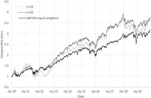
Monthly predictions from the random forest method play a major role in our research. In the first step, we present the results of naive portfolios created with random forest monthly predictions. As market capitalization does not impact the weights of our portfolios, we choose an equal-weighted benchmark consisting of all stocks from the S&P500, rebalanced monthly. Table 1 presents the equal-weighted portfolios that deliver higher returns for the cost of higher risk in comparison to the benchmark. As a result, both risk-adjusted performance measures (the Sharpe and Calmar ratios) are worse than the benchmark’s. A portfolio consisting of 50 stocks reaches the Sharpe ratio of 0.82, which is close to the benchmark’s 0.84. The difference between the Calmar ratio is higher (0.46 vs. 0.55). Figure 1 visualizes these relationships.

Figure 1. Equal-Weighted Portfolios vs. SPX500 Equal-Weighted.

This figure presents a line plot between the compounded rate of return and dates. The lines show the compounded total return of two equal-weighted portfolios consisting of 10 stocks (n = 10) and 50 stocks (n = 50) vs. the compounded total return of the equal-weighted S&P500 index. The sample period runs from 01/01/2010 to 31/12/2019.

Source: The Authors.

3.2. The optimum length of historical data as an input for the mean-variance optimizer

We start the empirical study on optimizers with a search for the optimum number of days that should be used to calculate the covariance matrix for the mean-variance optimizer. Additionally, we examine the HRP optimizer’s performance depending on the length of input data. Figure 2 visualizes the differences in the Sharpe ratio of portfolios constructed by the mean-variance and HRP optimizers that use 1–3 years of daily historical prices that are not high. The biggest difference appears between small portfolios consisting of 25 stocks. In this case, according to data from Table 2, the mean-variance portfolio with 3 years of daily prices generates a Sharpe ratio that is 5% better than a portfolio with 2 years of prices and 13% higher in comparison to the portfolio with 1 year of prices. We can see similar relationships with the smallest portfolio when using the HRP optimizer. However, this relationship stops working for portfolios built with additional stocks. The broken line, which represents a portfolio built with an optimizer fed with 2 years of daily prices, tends to situate over the other lines for most portfolios. For portfolios constructed with 100, 200, 225, and 250 stocks, the broken line lies above the others. In the case of the HRP optimizer, the differences in the Sharpe ratio for 2 or 3 years of historical daily prices are not important. It seems to be irrelevant to the HRP if the input history covers 2 or 3 years of historical daily prices.

Figure 2. Optimized Portfolio Performance Depending on the Length of Historical Data.

This figure presents line plots between the Sharpe or Calmar ratios and the number $n$ of stocks in portfolios. The two upper subfigures present the Sharpe ratio on the vertical axis. The two lower subfigures present the Calmar ratio on the vertical axis. The two subfigures on the left demonstrate ratios for the mean-variance (MV) optimized portfolios. The two subfigures on the right demonstrate ratios for the HRP (HRP) optimized portfolios. Optimizers fed with $d=365$ daily historical data are marked as 1-year history. Optimizers fed with $d=2*365$ daily historical data are marked as 2-year history. Optimizers fed with $d=3*365$ daily historical data are marked as 3-year history. The sample period runs from 01/01/2010 to 31/12/2019. The data covers stocks from the S&P500 index.

Source: The Authors.

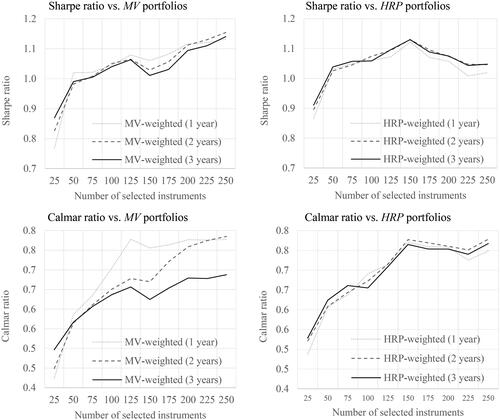
We can confirm our observations about the optimum length of data fed to the optimizer with the Calmar ratio. In this case, the mean-variance optimizer prefers 1 year of historical prices, while the HRP is not relatively sensitive, preferring 2 years. For larger portfolios, the Calmar ratio takes the highest values with 2 years of prices confirming the base relationship found with the Sharpe ratio.

Finally, we conclude that the optimum length of daily prices for the mean-variance optimizer is 2 years. Data with a shorter timespan might be problematic in the case of portfolios built with a smaller number of stocks ($n=25$). On the other hand, data with a longer timespan might present some old price correlations that are no longer valid and misrepresent the present stock price relationships. This can reduce the mean-variance optimizer’s efficiency for portfolios built with a large number of stocks ($n\ge 150$). In the case of HRP, it is not that important if we choose 1, 2, or 3 years of historical input. To stay constant with the length of input data in the research, we take 2 years as the best choice for both optimizers.

3.3. Optimized portfolios vs. the 1/n rule

Figure 3 visualizes how different portfolio creation techniques impact the Sharpe and Calmar ratios. Equal-weighted portfolios achieve the worst results measured with the Sharpe ratio. Table 2 shows that in the case of equal-weighted portfolios, the highest Sharpe ratio is achieved for portfolios consisting of $n=150$ and $n=200$ stocks with a value of 0.94. This is in contrast to the traditional approach where equal-weighted portfolios are commonly used for machine learning portfolio creation (Gu et al., 2020; Rasekhschaffe & Jones, 2019).

Figure 3. Portfolio Performance Depending on Creation Technique.

This figure presents line plots between Sharpe or Calmar ratios and the number $n$ of stocks in portfolios. The left subfigure presents the Sharpe ratio on the vertical axis. The right subfigure presents the Calmar ratio on the vertical axis. The equal-weighted line represents portfolios built with the 1/N rule. The MV-weighted (2 years) line represents portfolios built with the mean-variance optimizer using 2 years of daily historical prices. The HRP-weighted (2 years) line represents portfolios built with HRP optimized using 2 years of daily historical prices. The S&P500 equal-weighted broken line represents an equal-weighted portfolio of all stocks from the S&P500 index. The S&P500 dotted line represents the market portfolio of the S&P500 index. Note that for S&P500 equal-weighted and S&P500, all index constituents are taken under consideration; thus, the horizontal axis representing the different number of stocks used to create a portfolio does not impact these constants.

Source: The Authors.

The best Sharpe ratio is achieved by the mean-variance optimizer. The optimizer creates a portfolio from $n=250$ stocks that reaches a Sharpe ratio equal to 1.15. The mean-variance optimizer enhances its results with a growing number of selected stocks. The bigger its degree of freedom, the better the results. The relative outperformance of the mean-variance optimizer over the HRP optimizer starts with $n=200.$ This is quite surprising taking into account that there are only 500 stocks in the S&P500 index. The mean-variance optimizer needs 40% of stocks from the index to show its best performance. With $n<200,$ the best portfolios are created by HRP. This technique reaches its highest peak performance for $n=150$ with a Sharpe ratio of 1.13. Despite the lower number of stocks required to build a high-quality portfolio, HRP strongly diversifies the portfolio and the sum of the highest 10 weights state only for 20.1% of the portfolio. In contrast, a mean-variance optimizer that uses $n=250$ stocks concentrates on the top 10 weights 76.6% of the portfolio. Finally, the average outperformance in terms of the Sharpe ratio of mean-variance and HRP optimized portfolios over equal-weighted ones is 16.5% and 18.0%, respectively.

A portfolio’s efficiency measured with the Calmar ratio presents very similar tendencies. Overall, the best results are demonstrated by the mean-variance optimizer for $n=250$ stocks. The HRP optimizer demonstrates almost the same results with the peak performance reached for $n=150$ stocks. The weakest performance is shown by naive diversification with a peak Calmar ratio that is worse by 25% in comparison to the mean-variance peak performance. From an average perspective, in terms of the Calmar ratio, mean-variance portfolios outperformed equal-weighted ones by 23.9% and HRP portfolios by 30.6%.

3.4. Optimized portfolios vs. benchmarks

Figure 3 presents the Sharpe and the Calmar ratios for an equal-weighted portfolio consisting of S&P500 stocks and for the S&P500 index. The Sharpe ratio for the equal-weighted portfolio index reaches 0.84. Only one portfolio constructed with the mean-variance optimizer gets a worse score ($n=25,$ Sharpe ratio equal to 0.83). The rest of the configurations bring much better results. On its peak performance, the mean-variance optimizer outperforms the equal-weighted portfolio index by 37%. This relationship is confirmed with the Calmar ratio where the maximum overperformance reaches 44%.

In the analyzed period, the S&P500 index outperformed its equal-weighted portfolio in terms of both the Sharpe and the Calmar ratios by 15% and 32%, respectively. However, this performance was not enough to match the efficiency of the mean-variance portfolio that reaches a better score by 18% in terms of the Sharpe ratio and by 8% in terms of the Calmar ratio at its peak performance. It is worth noting that HRP managed to beat the index performance, too. Thus, optimized portfolios showed considerably better results than their benchmarks.

4. Robustness and additional tests

We verify the robustness of our results with two modifications from the original methodology. First, we adjust the mean-variance optimizer configuration by changing the limit of maximum weight per single instrument from 10% to 5%. This change affects more diversified portfolios. Second, we change the input data for our study from the S&P500 stocks to companies listed in the STOXX600 index. Additionally, to present the meaning of random forest predictions to the mean-variance optimizer’s performance, we show the performance of portfolios optimized with historical returns. In other words, we change the source of the expected return of information from the random forest predictions to historical returns.

4.1. Verification of optimal length of historical data

In Section 3.2, we conclude that the optimum length of historical data that should be used to feed the mean-variance and HRP optimizers is 2 years. Figure C.1. in the Online Appendix demonstrates the performance of portfolios created with a mean-variance optimizer that has a constraint for the maximum share of a single stock in the portfolio at the 5% level (instead of 10%). The charts visualize similar tendencies to the basic setting (see Figure 2). The broken line that represents the mean-variance optimizer fed with 2 years of historical daily stock prices tends to be situated above the other lines. Table C.1. in the Online Appendix shows precise numbers for each of the portfolios. In terms of the Sharpe ratio, a mean-variance optimizer that uses 2 years of historical data performs best for portfolios built with 100 to 250 stocks (which is 7 out of 10 configurations). In terms of the Calmar ratio, the performance of a mean-variance optimizer fed with 2 years of historical data is similar to that with 1 year of data and significantly better than for the optimizer using the longest timeframe. Therefore, the study on a more diversified optimizer (with a 5% limit) confirms our base findings that we should use 2 years of historical daily prices to feed the mean-variance optimizer.

Figure C.2. in the Online Appendix presents the performance of portfolios created with stocks from the STOXX600 index. The two subfigures on the left concentrate on the mean-variance optimizer. This time, the broken lines that represent the mean-variance optimizer fed with 2 years of historical daily prices lie very close to the continuous line that represents the optimizer using 3 years of historical data. The shortest data feed, represented by the dotted line, is situated considerably lower. Slightly different relationships are demonstrated in the two subfigures on the right. It seems that the HRP optimizer prefers a shorter feed. This is in contrast to results obtained with stocks from the S&P500 index. Table C.2. in the Online Appendix presents detailed values of the portfolios’ performances created with the STOXX600 index.

In summary, our robustness check confirms that the mean-variance optimizer should be fed with 2 years of historical data. The HRP optimizer is more unstable with its data length preference: the S&P500 case with 1 year of historical data is the worst choice, whereas in the STOXX600 case, it is the best solution. Yet, in both cases, the differences in HRP performance are not major and for consistency with our research, we stay with 2 years of data for both the mean-variance and HRP optimizers.

4.2. The sensitivity of results to mean-variance configuration changes

In this section, we verify how two configuration parameters impact the mean-variance optimizer’s performance. First, we change the constraint for maximum weight in a single instrument from 10% to 5%. Second, we modify the data used as expected returns. In our base model, we use the random forest prediction as input for expected returns. We test how the optimizer performs if it uses 2 years of historical prices as a proxy for expected returns. Figure C.3. in the Online Appendix visualizes the Sharpe and Calmar ratios’ performances in portfolios optimized with the mean-variance optimizer and configured with three different settings.

The mean-variance optimizer that uses a 10% maximum weight reaches the best Sharpe ratios (illustrated in the continuous line). The broken line representing the optimizer with a 5% limit has a similar slope, but lies slightly under the continuous line. In contrast, the dotted line indicating an optimizer fed with historical returns as a proxy for expected return has a downward orientation. With portfolios of more than 50 stocks, it lies significantly under the other lines. The difference grows with the rising number of stocks used to build portfolios. A performance measured with the Calmar ratio confirms the relationships visualized with the Sharpe ratio.

The analysis of the results presented in Figure C.3. proves that the performance of the mean-variance optimizer is not highly sensitive to constraint by the maximum weight limit per single instrument. Depending on the investor’s preferences or investment policy, different limits can be chosen without any major impact on portfolio performance. On the other hand, when one decides to build optimized portfolios with machine learning predictions, the expected returns should be estimated with such predictions instead of historical prices. This choice has a major impact on the portfolios’ performances.

4.3. Optimized portfolios vs. the 1/n rule on data from the STOXX600 index

Finally, we verify how mean-variance optimization performs with a different dataset. We move our focus from the U.S. S&P500 index to the European STOXX600 index. We use the same factors to create the random forest predictions and follow the random forest configuration methodology described in Section 2.2.2. It is important to highlight that the factors we use are optimized from the U.S. stocks’ perspective (Fama & French, 2015; Gu et al., 2020; Welch & Goyal, 2008). Therefore, it is not surprising that the relative overperformance of our portfolios in comparison to the STOXX600 benchmark is smaller than in the case of the S&P500.

Figure C.4. in the Online Appendix demonstrates the performance of different portfolio creation techniques. The left subfigure concentrates on the Sharpe ratio. The black continuous line that represents the mean-variance optimized portfolios is situated significantly higher than the other continuous lines. Along with data from Table C.2. in the Online Appendix, the maximum Sharpe ratio for the mean-variance optimizer using 2 years of historical daily prices reaches 0.66 for $n$ = 100, 125, and 150 stocks used to create the portfolio. That is 16% more than the maximum performance for an equal-weighted portfolio (0.57), and 10% more than for the HRP optimizer using 2 years of data (0.60).⁶ Very similar tendencies are visualized on the left subfigure of Figure C.4 in the Online Appendix. The Calmar ratio performance measure confirms the relative strength of the mean-variance optimizer over other portfolio creation techniques.

5. Conclusions

Using the recent advances in predicting the cross-section of excess returns with the random forest machine learning tool, we perform a comparative analysis of different portfolio construction techniques. We use 20 years of historical data of stocks from the S&P500 index to train the random forest and prepare the out-of-sample predictions. We find that, on average, the mean-variance optimized portfolios outperform the 1/N portfolios by 16.5% in terms of the Sharpe ratio. This result is in opposition to common criticism towards mean-variance optimizers (DeMiguel et al., 2009; Kolm et al., 2014). In an extensive study on optimizers, DeMiguel et al. (2009) demonstrate that the traditional mean-variance optimizer measured with the Sharpe ratio underperforms an equal-weighted portfolio on average by 41.1%. It reached an outperformance by 5.0% for only 1 out of the 6 tested portfolios. Furthermore, none of the 11 other modified mean-variance optimizers, on average, outperform a naive, equal-weighted portfolio.

We confirm the sound results of optimized portfolios’ performances with the Hierarchical Risk Parity (HRP) optimizer that, on average, outperforms the equal-weighted portfolios by 18.0%. The differences in the performance of the mean-variance and HRP optimizers are not significant and depend mainly on the number of stocks used to create portfolios, where HRP prefers a smaller number of shares and the mean-variance prefers a larger one. In absolute terms, the mean-variance optimizer outperforms HRP. Our results are robust with stocks from the European STOXX600 index and with different settings for the mean-variance optimizer.

At the highest level, our findings demonstrate that optimizers are efficient tools that cooperate with machine learning predictions. In the studies on empirical asset pricing that uses machine learning, it is a common practice to create equal-weighted portfolios with $n$ stocks having the highest monthly predictions (Gu et al., 2020; Rasekhschaffe & Jones, 2019). Our research proves that with optimizers, we can enhance the performance of machine learning portfolios.

From the portfolio optimization theory perspective, we show that excess return forecasts derived from machine learning may help to overcome the well-identified problems of quadratic mean-variance optimizers connected with sensitivity to changes in the inputs. We find that mean-variance optimizers fed with machine learning predictions as expected returns build more efficient portfolios in terms of the Sharpe ratio compared to naive diversification. This finding is supported by the Calmar ratio observations.

Our research proposes a portfolio-creation methodology based on the random forest machine learning tool and one of two optimizers (the mean-variance or HRP). This methodology is effective in outperforming the market benchmark. While we test two different optimizers to weighted portfolios derived from a cross-section of expected returns, other methods such as the Bayesian approach to estimation error, moment restrictions, portfolio constraints, or optimal combinations of portfolios may also be applied for the same purpose (DeMiguel et al., 2009). For future studies, one may explore the effect of a wider set of optimizers used with a cross-section of expected excess returns, where an improved methodology may result in better efficiency measures. Another direction of further studies may be to search for further improvements in the predictions’ accuracy and volatility. Following Gu et al. (2020), we implement the random forest method to forecast excess returns, but potentially one can use other, more effective methods. Finally, it is worth verifying how this two-step methodology performs in different markets and after the impact of transaction costs.

Disclosure statement

No potential conflict of interest was reported by the authors.

Data availability statement

The data that support the findings of this study are available from Refinitiv. Restrictions apply to the availability of these data, which were used under license for this study. Data are available from the authors on request with the permission of Refinitiv.

Additional information

Funding

The project was financed within the Regional Initiative for Excellence programme of the Minister of Science and Higher Education of Poland, years 2019-2022, grant no. 004/RID/2018/19, financing 3,000,000 PLN.

Notes

1 Kolm et al. (2014) present some of the approaches developed to address the challenges encountered when using portfolio optimization in practice, including the sensitivity to the estimates of expected returns. In order to mitigate the impact of estimation errors in mean variance optimization, the following techniques are demonstrated: 1) constraints on portfolio weights (Jagannathan & Ma, 2003), 2) diversification measures (Bouchaud et al., 1997), 3) Bayesian techniques and the Black-Litterman model (Black & Litterman, 1992), 4) robust optimization (Goldfarb & Iyengar, 2003), and 5) incorporating higher moments and tail-risk measures (Rockafellar & Uryasev, 2000). Futhermore Tang et al. (2004) demonstrates different approaches to incorporate uncertainty in portfolio optimization categorized as stochastic uncertainy and fuzziness.

2 The empirical study on the mean-variance model and its extensions showed that none is consistently better than the 1/N rule in terms of the Sharpe ratio, certainty-equivalent return, or turnover (DeMiguel et al., 2009).

3 We follow the machine learning definition proposed by Gu et al. (2020). The full definition is: “(i) a diverse collection of high-dimensional models for statistical prediction, combined with (ii) so-called ‘regularization’ methods for model selection and mitigation of overfit, and (iii) efficient algorithms for searching among a vast number of potential model specifications.”

4 Gu et al. (2020) indicate 20 factors that have the biggest impact on the random forest method. Datastream provides data for 18 factors that explain around 90% of the model’s performance. Thus, 10% of unexplained performance is not problematic in the context of our research main objective, which is to prepare stable stock excess return predictions.

5 We look closely for any potential forward-looking bias. We conclude that the data from Revinitiv Datastream does not need to be time shifted. Note, however, that the verification of the time shifts is crucial for a prediction’s reliability. Another issue is missing characteristics. We remove monthly observations that lack both the closing price and 12-month rate of returns. We replace other gaps with the cross-sectional median.

6 As highlighted in Section 4.1., the HRP optimizer performs best with 1 year of historical data on stocks from the STOXX600 index. With 1 year of data, its maximum Sharpe ratio reaches 0.66, which is equal to the mean-variance optimizer’s maximum performance.

References

- Abraham, A., Nath, B., & Mahanti, P. K. (2001). Hybrid intelligent systems for stock market analysis. Lecture Notes in Computer Science (Including Subseries Lecture Notes in Artificial Intelligence and Lecture Notes in Bioinformatics), 2074, 337–345. https://doi.org/10.1007/3-540-45718-6_38
- Atsalakis, G. S., & Valavanis, K. P. (2009a). Forecasting stock market short-term trends using a neuro-fuzzy based methodology. Expert Systems with Applications, 36(7), 10696–10707. https://doi.org/10.1016/j.eswa.2009.02.043
- Atsalakis, G. S., & Valavanis, K. P. (2009b). Surveying stock market forecasting techniques – Part II: Soft computing methods. Expert Systems with Applications, 36(3), 5932–5941. https://doi.org/10.1016/j.eswa.2008.07.006
- Black, F., & Litterman, R. (1992). Global portfolio optimization. Financial Analysts Journal, 48(5), 28–43. https://doi.org/10.2469/faj.v48.n5.28
- Bouchaud, J.-P., Potters, M., & Aguilar, J.-P. (1997). Missing information and asset allocation. Science & Finance (CFM) working paper archive 500045, Science & Finance, Capital Fund Management. https://ideas.repec.org/p/sfi/sfiwpa/500045.html
- Breiman, L. (2001). Random forests. Machine Learning, 45(1), 5–32. https://doi.org/10.1023/A:1010933404324
- Breiman, L., Friedman, J. H., Olshen, R. A., & Stone, C. J. (1984). Classification and regression trees. Chapman & Hall.
- Clarke, R., De Silva, H., & Thorley, S. (2002). Portfolio constraints and the fundamental law of active management. Financial Analysts Journal, 58(5), 48–66. https://doi.org/10.2469/faj.v58.n5.2468
- Cochrane, J. H. (2011). Presidential address: discount rates. The Journal of Finance, 66(4), 1047–1108. https://doi.org/10.1111/j.1540-6261.2011.01671.x
- DeMiguel, V., Garlappi, L., & Uppal, R. (2009). Optimal versus naive diversification: How inefficient is the 1/N portfolio strategy? Review of Financial Studies, 22(5), 1915–1953. https://doi.org/10.1093/rfs/hhm075
- Fama, E. F., & French, K. R. (2015). A five-factor asset pricing model. Journal of Financial Economics , 116(1), 1–22. https://doi.org/10.1016/j.jfineco.2014.10.010
- Fama, E. F., & MacBeth, J. D. (1973). Risk, return, and equilibrium: empirical tests. Journal of Political Economy, 81(3), 607–636. In The University of Chicago Press. https://doi.org/10.2307/1831028 https://doi.org/10.1086/260061
- Frydman, H., Altman, E. I., & Kao, D.-L. (1985). Introducing recursive partitioning for financial classification: the case of financial distress. The Journal of Finance, 40(1), 269–291. https://doi.org/10.2307/2328060
- Goldfarb, D., & Iyengar, G. (2003). Robust portfolio selection problems. Mathematics of Operations Research, 28(1), 1–38. https://doi.org/10.1287/moor.28.1.1.14260
- Gu, S., Kelly, B., & Xiu, D. (2020). Empirical asset pricing via machine learning. The Review of Financial Studies, 33(5), 2223–2273. https://doi.org/10.1093/rfs/hhaa009
- Harvey, C. R., Liu, Y., Zhu, H. (2016). … and the cross-section of expected returns. Review of Financial Studies, 29(1), 5–68. https://doi.org/10.1093/rfs/hhv059
- Jagannathan, R., & Ma, T. (2003). Risk reduction in large portfolios: why imposing the wrong constraints helps. The Journal of Finance , 58(4), 1651–1683. In ( Issue John Wiley & Sons, Ltd. https://doi.org/10.1111/1540-6261.00580
- Kao, D. L., & Shumaker, R. D. (1999). Equity style timing. Financial Analysts Journal, 55(1), 37–48. Issue CFA Institute. https://doi.org/10.2469/faj.v55.n1.2240
- Kolm, P. N., Tütüncü, R., & Fabozzi, F. J. (2014). 60 Years of portfolio optimization: Practical challenges and current trends. European Journal of Operational Research, 234(2), 356–371. https://doi.org/10.1016/j.ejor.2013.10.060
- Ledoit, O., & Wolf, M. (2003). Improved estimation of the covariance matrix of stock returns with an application to portfolio selection. Journal of Empirical Finance, 10(5), 603–621. https://doi.org/10.1016/S0927-5398(03)00007-0
- Lintner, J. (1965). Security prices, risk, and maximal gains from diversification. The Journal of Finance, 20(4), 587. https://doi.org/10.2307/2977249
- López de Prado, M. (2016). Building diversified portfolios that outperform out of sample. The Journal of Portfolio Management, 42(4), 59–69. https://doi.org/10.3905/jpm.2016.42.4.059
- Markowitz, H. (1952). Portfolio selection. The Journal of Finance, 7(1), 77. https://doi.org/10.2307/2975974
- Miller, K. L., Li, H., Zhou, T. G., & Giamouridis, D. (2015). A risk-oriented model for factor timing decisions. The Journal of Portfolio Management, 41(3), 46–58. https://doi.org/10.3905/jpm.2015.41.3.046
- Miller, K. L., Ooi, C., Li, H., & Giamouridis, D. (2013). Size rotation in the U.S. equity market. The Journal of Portfolio Management, 39(2), 116–127. https://doi.org/10.3905/jpm.2013.39.2.116
- Mossin, J. (1966). Equilibrium in a capital asset market. Econometrica, 34(4), 768. https://doi.org/10.2307/1910098
- Naveed Jan, M., & Ayub, U. (2019). Do the fama and french five-factor model forecast well using ANN? Journal of Business Economics and Management, 20(1), 168–191. https://doi.org/10.3846/jbem.2019.8250
- Pantazopoulos, K. N., Tsoukalas, L. H., Bourbakis, N. G., Brün, M. J., & Houstis, E. N. (1998). Financial prediction and trading strategies using neurofuzzy approaches. IEEE Transactions on Systems, Man, and Cybernetics. Part B, Cybernetics : a Publication of the IEEE Systems, Man, and Cybernetics Society, 28(4), 520–531. https://doi.org/10.1109/3477.704291
- Rasekhschaffe, K. C., & Jones, R. C. (2019). Machine learning for stock selection. Financial Analysts Journal, 75(3), 70–88. https://doi.org/10.1080/0015198X.2019.1596678
- Rockafellar, R. T., & Uryasev, S. (2000). Optimization of conditional value-at-risk. The Journal of Risk, 2(3), 21–41. https://doi.org/10.21314/JOR.2000.038
- Sharpe, W. F. (1964). Capital asset prices: a theory of market equilibrium under conditions of risk. The Journal of Finance, 19(3), 425. https://doi.org/10.2307/2977928
- Sorensen, E. H., Miller, K. L., & Ooi, C. K. (2000). The decision tree approach to stock selection. The Journal of Portfolio Management, 27(1), 42–52. https://doi.org/10.3905/jpm.2000.319781
- Tang, J., Wang, D. W., Fung, R. Y. K., & Yung, K.-L. (2004). Understanding of fuzzy optimization: theories and methods. Journal of Systems Science and Complexity, 17(1), 117–136.
- Welch, I., & Goyal, A. (2008). A comprehensive look at the empirical performance of equity premium prediction. Review of Financial Studies, 21(4), 1455–1508. https://doi.org/10.1093/rfs/hhm014