Machine learning methods based on probabilistic decision tree under the multi-valued preference environment

Abstract

In the classification calculation, the data are sometimes not unique and there are different values and probabilities. Then, it is meaningful to develop the appropriate methods to make classification decision. To solve this issue, this paper proposes the machine learning methods based on a probabilistic decision tree (DT) under the multi-valued preference environment and the probabilistic multi-valued preference environment respectively for the different classification aims. First, this paper develops a data pre-processing method to deal with the weight and quantity matching under the multi-valued preference environment. In this method, we use the least common multiple and weight assignments to balance the probability of each preference. Then, based on the training data, this paper introduces the entropy method to further optimize the DT model under the multi-valued preference environment. After that, the corresponding calculation rules and probability classifications are given. In addition, considering the different numbers and probabilities of the preferences, this paper also uses the entropy method to develop the DT model under the probabilistic multi-valued preference environment. Furthermore, the calculation rules and probability classifications are similarly derived. At last, we demonstrate the feasibility of the machine learning methods and the DT models under the above two preference environments based on the illustrated examples.

Keywords:

• Machine learning method
• probabilistic decision tree
• multi-valued preference
• decision making

JLE CLASSIFICATIONS:

• G15
• G11
• G10

1. Introduction

With the development of artificial intelligence, machine learning plays a vital role in it. Machine learning is used in addressing data set containing a lot of messy information (Blum & Langley, 1997), and it can be widely applied in various fields, such as the sales (Sun et al., 2008; Tsoumakas, 2019; Wong & Guo, 2010), the credit assessment (Kruppa et al., 2013; Pal et al., 2016), and the autonomous vehicles (Qayyum et al., 2020), etc. Moreover, machine learning is commonly be divided into two different types including the unsupervised learning and the supervised learning. The unsupervised learning is a method that classifies samples through data analysis of a large number of samples without the category information (Barlow, 1989; Goldsmith, 2001). The most common unsupervised learning algorithm is the k-means method (Capó et al., 2020; Han et al., 2020). The supervised learning is a kind of method to learn a function from a given training data. Next, when new data comes, it can predict the result based on the former function (Figueiredo, 2003; Gerfo et al., 2008). The supervised learning contains many algorithms, such as the decision tree (DT) (Pal & Mather, 2003; Polat & Güneş, 2007), the k-nearest neighbor (Zhang & Zhou, 2007; Lee et al., 2019), the random forests (Mantas et al., 2019), and the support vector machines (Utkin, 2019; Yuan et al., 2010). Obviously, we can conclude that the machine learning method is not only widely used but also has many kinds of extended algorithms. Based on this, the machine learning method can be developed by fusing some new conditions according to the actual requirements.

In the above machine learning methods, the DT is a basic machine learning classification, regression (Galton, 1889), and data mining (Han & Micheline, 2006) method. Hunt (1965) proposed the Concept Learning System (CLS) which introduces the concept of the DT. Based on the ID3 algorithm, the DT was formally proposed and defined (Quinlan, 1986, 1987). After that, some scholars continued to research and improve this method based on the ID3 algorithm, resulting in many classic classification algorithms such as the CART (Crawford, 1989; Rutkowski et al., 2014), the C4.5 (Quinlan, 1996), and the SLIQ (Narasimha & Naidu, 2014). In addition, these methods have a large number of extended applications (Bhargava et al., 2013; Hardikar et al., 2012; Ruggieri, 2002; Santhosh, 2013). Although the above algorithms with inductive properties used to construct the DTs can make classification and regression in the single-valued attributes environment, the operation results are not satisfactory when the environment changes (Chen et al., 2003).

According to the above analysis, the multi-valued concept and the multi-valued environment were presented (Miao & Wang, 1997). Some scholars built the models by using the similarity (Clarke, 1993; Santini & Jain, 1999; Tversky,1977) to solve the problem under the defined multi-valued and multi-labeled environments (Chen et al., 2010; Cheng, 2014; Chou & Hsu, 2005; Hsu, 2021; Yi et al., 2011; Zhao & Li, 2007). Obviously, they realized the transition from the single-valued to the multi-valued environments. This lays a research foundation for the proposal of a decision classification algorithm under the multi-valued preference environment. However, in the decision-making process, the numbers and weights of the preferences are sometimes different. Therefore, it also provides a research direction for this paper to extend the multi-valued preference environment to the probabilistic multi-valued preference environment.

To achieve the above aims, this paper is organized as follows: This paper briefly reviews the traditional DT models in Section 2. The weight and quantity matching method and the DT algorithm under the multi-valued preference environment are proposed in Section 3. In Section 4, we further propose a machine learning model under the probabilistic multi-valued preference environment and demonstrate the operation process with an example. Section 5 gives the derived conclusions.

2. Preliminaries

The concept of the probabilistic multi-valued attributes environment can be divided into two perspectives to understand. The first perspective is the environment with the multi-valued preferences; the second perspective is the environment with the probabilistic multi-valued preferences. It is found that both of these environments are established based on the traditional single-valued attributes environment. Therefore, before introducing the two new environments in detail, we first briefly review machine learning in the traditional single-valued attributes environment. Then, this paper introduces the construction process of the DT model under the traditional single-valued attributes environment. Finally, we describe the multi-valued and probabilistic multi-valued preference environments. By comparing the three environments through examples, this paper can intuitively present the changes.

2.1. The DT model in a traditional single-valued attributes environment

The traditional DTs include the ID3, C4.5, and CART methods. In this paper, the ID3 algorithm is selected as the basic technique. This method uses the entropy method and information gain to construct a DT, where the information gain is the difference between the information entropy and conditional entropy, and then selects the attribute with the largest information gain as the optimal attribute to form a classification node. The main construction steps of the DT model are shown below:

Assume that a training data set is $S$ where $\left|S\right|$ denotes the sample number, and these samples have $K$ classes labeled $C_k,$ $k=1,2,3,\dots ,K,$ and $\left|C_k\right|$ represents the number of samples belonging to the class $C_k.$ If a discrete attribute $A$ has $m$ possible values, and then $A$ divides the training data set $S$ into $D$ training data subsets and each training data subset can be labeled as $S_d\mathrm{}\mathrm{(}d=1,2,\dots ,D),$ where $\left|S_d\right|$ is the number of samples in $S_d.$ Note that the set $S_{dk}$ belongs to the class $C_k$ in the subset $S_d$ and $\left|S_{dk}\right|$ is its sample number of $S_{dk}.$ The corresponding calculation formula of the information gain is given as follows: (1) $$\mathit{Gain}(S,A)=\mathit{Info}(S)-\mathit{Info}(S/A)$$(1)

Eq. (1)(1) $$\mathit{Gain}(S,A)=\mathit{Info}(S)-\mathit{Info}(S/A)$$(1) denotes the information gain of the attribute $A$ in the training data set $S,$ it is used to measure the degree of information uncertainty reduction.

Eq. (2)(2) $$\mathit{Info}(S)=-{\sum }_{k=1}^K\frac{\left|C_k\right|}{\left|S\right|}{\hspace{0.17em}\text{log}\hspace{0.17em}}_2\frac{\left|C_k\right|}{\left|S\right|}$$(2) represents the information entropy of the training set $S.$ (2) $$\mathit{Info}(S)=-{\sum }_{k=1}^K\frac{\left|C_k\right|}{\left|S\right|}{\hspace{0.17em}\text{log}\hspace{0.17em}}_2\frac{\left|C_k\right|}{\left|S\right|}$$(2)

Eq. (3)(3) $$\mathit{Info}(S/A)=-{\sum }_{d=1}^D\frac{\left|S_d\right|}{\left|S\right|}{\sum }_{k=1}^K\frac{\left|S_{dk}\right|}{\left|S_d\right|}{\hspace{0.17em}\text{log}\hspace{0.17em}}_2\frac{\left|S_{dk}\right|}{\left|S_d\right|}.$$(3) denotes the conditional entropy of the attribute $A$ in the training data set $S.$ Generally, the classification ability of an attribute is enhanced with the increase of the information gain. Then, we can select the attribute with the largest information gain as the optimal attribute. (3) $$\mathit{Info}(S/A)=-{\sum }_{d=1}^D\frac{\left|S_d\right|}{\left|S\right|}{\sum }_{k=1}^K\frac{\left|S_{dk}\right|}{\left|S_d\right|}{\hspace{0.17em}\text{log}\hspace{0.17em}}_2\frac{\left|S_{dk}\right|}{\left|S_d\right|}.$$(3)

According to this idea, this paper traverses the entire training data set and finds out all the attributes to construct the probabilistic DT. Note that the study in this subsection is only based on the traditional single-valued attributes environment, and then we study the multi-valued and probabilistic multi-valued preference environment in the next section.

2.2. The multi-valued and probabilistic multi-valued preference environment

As we know, there are some situations which show the multi-valued preference and probabilistic multi-valued preference characters in real life. However, few models are developed based on the multi-valued and probabilistic multi-valued preference environments. Therefore, we try to study these two new environments and propose the feasible probabilistic classification and machine learning models in this paper.

It is noted that the original data are derived from the DT cases (Quinlan, 1987). Tables 1–3 respectively represent the above three environments in this reference. We can find that there are four attributes in each table, namely “outlook, temperature, humidity, windy”. Each attribute has its sub attributes. For example, “outlook” contains three sub attributes of “sunny, overcast, rain”; “humidity” contains three sub attributes of “hot, mild, cool”; “temperature” contains two sub attributes “high, normal”, and “windy” contains two sub attributes “true, false”. Among them, $D_i$ denotes the sample of day $i.$ The attributes “outlook, temperature, humidity, windy” means that there are four attributes in the data set; each attribute contains different sub attributes such as “sunny, overcast, rain”. According to these setting, we have $o_{ij},$ $t_{ij},$ $h_{ij},$ and $w_{ij}$ represent the probability values of the $j$ th attribute in the $i$ th sample. Classes $P$ and $N$ represent the positive and negative instances. $p_i$ and $1-p_i$ denote the probability values of $P$ and $N$ in the $i$ th sample. Therefore, we can further describe these three environments in detail.

Table 1. A single-valued preference sample.

No.	Attributes				Class P/N
	Outlook	Temperature	Humidity	Windy
$D11$	rain	mild	normal	false	$P$
$D12$	rain	cool	normal	true	$N$
$D13$	overcast	hot	high	false	$P$

Source: The Authors.

Table 1 shows a single-value preference environment. Extract sample $D13$ from Table 1 as an illustration, we can find that $D13$ shows each attribute only retains one attribute value as the final state. For example, the attribute “outlook” selects the attribute of “overcast”, “temperature” selects the attribute of “hot”, “humidity” selects the attribute of “high”, and “windy” selects the attribute of “false”. In this single-valued preference environment, each rule corresponds to only one classification result $P$ or $N,$ which is called the absolute classification.

Table 2 shows a multi-valued preference environment. We can find that the preference values of the sample have the multi-valued forms. Take the sample $D23$ in Table 2 as an illustrated example, $D23$ shows that its each attribute contains one or more preferences. In this example, the attribute “outlook” selects three preferences, namely “overcast, sunny, rain”, which means that three different preferences of “outlook” appeared on this day. Obviously, this situation is common in real life. In this paper, we focus on these three preferences but not the order that they occur. Based on this, a multi-valued preference environment can be shown as follows:

Table 2. A multi-valued preference sample.

No.	Attributes				Class P/N
	Outlook	Temperature	Humidity	Windy
$D21$	rain	mild	normal	false	$(p_{21},1-p_{21})$
$D22$	rain, overcast	cool, hot	normal, high	true	$(p_{22},1-p_{22})$
$D23$	overcast, sunny, rain	hot, mild, cool	high	false, true	$(p_{23},1-p_{23})$

Source: The Authors.

Definition 1. Let $D_i$ be the $i$ th sample with $j$ attributes, and each attribute contains $t$ preferences, and then this case can be defined as the multi-valued preference environment, where the probability of each preference is equal, $i=1,2,\dots ,n,$ $j=1,2,\dots ,m,$ and $t=1,2,\dots ,l.$

According to Def. 1, we can obtain the multi-valued preference environment. Then, it is found that all the attributes in the data retain the single and multiple preferences. The weight of each preference in the same sample and the same attribute is equal. Furthermore, we can find that the probability of preference is not involved here.

Table 3 shows the multi-valued preference environment with the probability. Taking $D33$ in Table 3 as an example, we can find that this is different from Table 2 and each preference have their probability. Moreover, $O,$ $T,$ $H,$ and $W$ respectively represent the possible probabilities. Taking the attribute “temperature” in $D33$ as an example, this shows that the occurrence probability of preference “hot” is $t_{31},$ “mild” is $t_{32},$ and “cool” is $t_{33}$ on the same day, and the sum of the probabilities of these three preferences is 1.

Table 3. A probabilistic multi-valued preference sample.

No.	Attributes				Class P/N
	Outlook	Temperature	Humidity	Windy
$D31$	rain $o_{13}$	mild $t_{12}$	normal $h_{12}$	false $w_{12}$	$(p_{31},1-p_{31})$
$D32$	overcast, rain $o_{22},o_{23}$	hot, cool $t_{21},t_{23}$	high, normal $h_{21},h_{22}$	true $w_{21}$	$(p_{32},1-p_{32})$
$D33$	sunny, overcast, rain $o_{31},o_{32},o_{33}$	hot, mild, cool $t_{31},t_{32},t_{33}$	high $h_{31}$	true, false $w_{31},w_{32}$	$(p_{33},1-p_{33})$

Source: The Authors.

Moreover, the attribute “humidity” just has one attribute value “high”. Obviously, the occurrence probability of the attribute value “high” in this day can be set as 100%, and the occurrence probability of the other attribute “normal” can be set as 0%. Finally, by observing the three small samples in Table 3, we can find that the number of attribute in each sample can be set as the different values, which means that the attribute situation that occurs every day is also different. We think that this situation including the multi-valued preference and its probability is closer to real life.

The three different environments aforementioned are three kinds of presentations and show the different relationships. The multi-valued preference is a development of the single-valued attribute, while the probabilistic multi-valued preference is a development of the multi-valued preference. Therefore, this paper develops the DT model based on these different environments and analyzes them according to these two situations which are the main innovations of this paper.

3. The machine learning model in the multi-valued preference environment

As aforementioned in Section 2.1, the ID3 algorithm is used to calculate the single-valued discrete data. Then, this method directly selects the optimal attribute by calculating their information gains and constructs the machine learning model. The hypothesis of the ID3 algorithm is that the weight of each sample in each column of attributes is 1. However, the multi-valued and probability multi-valued data sets studied in this paper have the main characteristics, which are the different numbers of attribute values in the same attribute and sample. Thus, these two types of data cannot be directly embedded in the information gain formula to select the optimal attribute in the calculation process.

With respect to the above discussion, we can find that the build of the DT in the multi-valued preference environment includes two main steps. The first step is to solve the aforementioned problem by preprocessing the original training data. In this step, the numbers and weights of the preferences in the original training data should be re-matched to balance them. The second step is to construct a DT using the new training data. Compare with the optimal degree of each attribute and its preference based on the bifurcation criterion, we can find that the optimal attribute is different. Based on this, we first propose the weight and quantity matching method under the multi-valued preference environment in the next subsection.

3.1. The weight and quantity matching in the multi-valued preference environment

In the multi-valued preference environment, the training data set $S$ contains $n$ samples for the multi-dimensional attributes which presents a multi-dimensional matrix. Suppose the attribute $A$ in $i$ th sample contains $l$ preferences can be expressed as $\left\{a_{i1},a_{i2},\dots ,a_{il}\right\}.$ Then, the preferences that are selected for the attribute $A$ in the training data set $S$ can be shown as a matrix below: $$S^A=\left[\begin{array}{c}{a}_{11},a_{12},a_{13},\dots ,a_{1l}\\ a_{21},a_{22},a_{23},\dots ,a_{2l}\\ \dots \\ a_{n1},a_{n2},a_{n3},\dots ,a_{nl}\end{array}\right].$$ where $S^A$ represents a matrix includes the different preferences in the attribute $A$ of all the samples, which is a combination of the $n$ sets $\{a_{i1},a_{i2},a_{i3},\dots ,a_{il}\}$ and $i=1,2,\dots ,n.$ $a_{it}$ denotes the $i$ th sample selects the $t$ th preference in the attribute $A$ and $t=1,2,\dots ,l,$ $\left|a_{it}\right|$ is defined as the weight of the preference $a_{it}.$ Moreover, let $L_i$ denotes the number of preferences belonging to the attribute $A$ in the $i$ th sample. However, since each sample exists independently, each $L_i$ can be unequal. Therefore, different preferences have different weights under the attribute $A.$

To address the issue of uneven weights caused by the unequal numbers, this paper proposes a weight and quantity matching method. This method is to use the least common multiple to match the quantity of data. This principle of the least common multiple can change the amounts of data into the same one. Assume the least common multiple is marked $\theta =〚〛.$ In this multi-valued training data set $S,$ the least common multiple of the attribute $A$ can be calculated as $\theta =〚L_1,L_2,L_3,\dots ,L_n〛.$ The original training data set $S$ can be expanded accordingly and the expansion multiple is marked with $\theta /L_i.$ Here, we make the number of preferences in each sample with respect to the attribute $A$ become $\theta .$ Therefore, the weight reduction of each preference is a multiple of $1/L_i$ where $1/L_i=\frac{\theta }{L_i}/\theta .$ Similarly, the preferences of other attributes can also obtain new weights using the given weight and quantity matching method. Then, we can get a new multi-valued preference data set $S^{\prime },$ and assume $\left|a_{it}\right|/L_i\mathrm{}(i=1,2,\dots ,n;\mathrm{}t=1,2,\dots ,l)$ as the new weight of each preference.

Based on this, we finish the process of quantity matching and give a weight and quantity matching method. Therefore, we complete the weight and quantity matching in the multi-valued preference environment. Further, we can analyze how to use the weight and quantity matching method to develop the DT algorithm under the multi-valued preference environment.

3.2. The DT algorithm in the multi-valued preference environment

As we know, the DT model under the single-valued environment uses the information gain to select bifurcation nodes. Similarly, under the multi-valued attribute environment, we also construct the DT model based on the bifurcation nodes. However, with respect to the different environments, the selection criterion for the bifurcation nodes are changed accordingly. In this paper, we develop a new method of selecting nodes under the multi-valued preference environment as the bifurcation criterion.

The following content explains these concepts in conjunction with the mathematical expressions and modeling process of the new DTs and machine learning. We also introduce the notations that are used in the following Sections, which are shown in Table 4.

Table 4. The main notations in the multi-valued preference environment.

Notations	Introduction	Notations	Introduction
$S^{\prime }$	The training data set after quantity matching	$1/L_i$	The multiple of preferences $a_{iw}$ that should be reduced after quantity matching
$\left|S^{\prime }\right|$	The sample number of $S^{\prime }$	$1/L_{ik}$	The multiple of preferences $a_{\mathit{iwk}}$ that should be reduced after quantity matching
$A$	The attribute of $S^{\prime }$	$1/R_i^c$	The multiple of preferences $a_{iu}^c$ that should be reduced after quantity matching
$\left|C_k\right|$	The sample number of the class $C_k$	$1/R_{ik}^c$	The multiple of preferences $a_{\mathit{iuk}}^c$ that should be reduced after quantity matching
$\left|a_{iw}\right|$	The weight about the $w$ th preference of the root node attribute in the $i$ th sample	$P_{iw}^Z(b)$	The preferences $a_{iw}$ of the root node attribute is under branch $Z,$ where there are $b$ samples with classification result $P$
$\left|a_{\mathit{iwk}}\right|$	The weight about the $w$ th preference in the root node attribute belongs to the class $k$ in the $i$ th sample	$P_{\mathit{icu}}^Z(b)$	The preference $a_{iu}$ of the $c$ th sub node is under branch $Z,$ where there are $b$ samples with classification result $P$
$\left|a_{iu}^c\right|$	The weight about the $u$ th preference of the sub node attribute $c$ in the $i$ th sample	$N_{iw}^Z(g)$	The preference $a_{iw}$ of the root node attribute is under branch $Z,$ where there are $g$ samples with classification result $N$
$\left|a_{\mathit{iuk}}^c\right|$	The weight about the $u$ th preference of the sub node attribute $c$ belongs to class $k$ in the $i$ th sample	$N_{\mathit{icu}}^Z(g)$	The preference $a_{iu}$ of the $c$ th sub node is under branch $Z,$ where there are $g$ samples with classification result $N$

Source: The Authors.

Due to the different environments, this paper optimizes the algorithm in the single-valued preference environment and improves the information gain as a bifurcation criterion that can handle the multi-valued preferences. Moreover, this paper divides the node selection into two steps, which are the selection of the root node and the other nodes. The reason is that the selection of the root node only considers the changing relationship between the preference and classification. However, the selection of other nodes needs to be based on the known conditions of the previous node. Therefore, the weight modification should be considered, as well as the previous node's weights.

With respect to these principles, the calculation of the root node bifurcation criterion in the multi-valued preference environment is summarized as follows: (4) $$M_r\left(S^{\prime },A\right)=bi{f}_r\left(S^{\prime }\right)-co{n}_r\left(S^{\prime }/A\right)$$(4)

Then, the bifurcation information entropy $bi{f}_r(S^{\prime })$ of the root node is shown as (5) $$bi{f}_r\left(S^{\prime }\right)=-{\sum }_{k=1}^K\frac{\left|C_k\right|}{\left|S^{\prime }\right|}{\hspace{0.17em}\text{log}\hspace{0.17em}}_2\frac{\left|C_k\right|}{\left|S^{\prime }\right|}\mathrm{ }\mathrm{ }$$(5)

Furthermore, the conditional information entropy of the root node is presented as follows: (6) $$co{n}_r\left(S^{\prime }/A\right)\mathrm{ }\mathrm{ }=-\sum _{i=1}^n\left[\sum _{w=1}^W\frac{\left|a_{iw}\right|.\frac{1}{L_i}}{\left|S^{\prime }\right|}\left(\frac{\sum _{k=1}^K\left|a_{\mathit{iwk}}\right|.\frac{1}{L_{ik}}}{\left|a_{iw}\right|.\frac{1}{L_i}}{\hspace{0.17em}\text{log}\hspace{0.17em}}_2\frac{\sum _{k=1}^K\left|a_{\mathit{iwk}}\right|.\frac{1}{L_{ik}}}{\left|a_{iw}\right|.\frac{1}{L_i}}\right)\right]$$(6)

Similarly, the calculation of the sub node bifurcation criterion in the multi-valued preference environment is summarized as follows: (7) $$M_{\mathit{sub}}\left(S^{\prime },A\right)=bi{f}_{\mathit{sub}}\left(S^{\prime }\right)-co{n}_{\mathit{sub}}\left(S^{\prime }/A\right)$$(7)

Then, the bifurcation information entropy $bi{f}_{\mathit{sub}}(S_w^{\prime })\mathrm{}(w=1,2,\dots ,W)$ of the sub node is (8) $$bi{f}_{\mathit{sub}}\left(S_w^{\prime }\right)\mathrm{ }\mathrm{ }=-\sum _{i=1}^n\sum _{k=1}^K\frac{\left|a_{\mathit{iwk}}\right|.\frac{1}{L_{ik}}}{\left|a_{iw}\right|.\frac{1}{L_i}}{\hspace{0.17em}\text{log}\hspace{0.17em}}_2\frac{\left|a_{\mathit{iwk}}\right|.\frac{1}{L_{ik}}}{\left|a_{iw}\right|.\frac{1}{L_i}}$$(8)

Moreover, the conditional information entropy of the sub node is presented as (9) $$co{n}_{\mathit{sub}}\left(S_{wc}^{\prime }/A\right)\mathrm{ }\mathrm{ }=-\sum _{i=1}^n\frac{{\prod }_{u=1}^U(\left|a_{iw}\right|.\frac{1}{L_i}.\left|a_{iu}^c\right|.\frac{1}{R_i^c})}{\left|a_{iw}\right|.\frac{1}{L_i}}\cdot \left(\frac{{\sum }_{k=1}^K(\left|a_{iw}\right|.\frac{1}{L_i}.{\prod }_{u=1}^U\left|a_{\mathit{iuk}}^c\right|.\frac{1}{R_{ik}^c})}{\left|a_{iw}\right|.\frac{1}{L_i}.{\prod }_{u=1}^U\left|a_{iu}^c\right|.\frac{1}{R_i^c}}{\hspace{0.17em}\text{log}\hspace{0.17em}}_2\frac{{\sum }_{k=1}^K(\left|a_{iw}\right|.\frac{1}{L_i}.{\prod }_{u=1}^U\left|a_{\mathit{iuk}}^c\right|.\frac{1}{R_{ik}^c})}{\left|a_{iw}\right|.\frac{1}{L_i}.{\prod }_{u=1}^U\left|a_{iu}^c\right|.\frac{1}{R_i^c}}\right)$$(9)

Therefore, we can obtain the root node and sub node bifurcation criterion in the multi-valued preference environment. As we know, after the numbers of attributes are matched, the preference weights can be changed. When calculating the bifurcation criterion values of the nodes, the previous nodes should be considered again. Generally, the larger bifurcation criterion, the more information contained in the data, and the greater uncertainty.

However, the classification result of the DT can be not accurate at this stage and the same attribute branch can appear the different classification results. Then, the final result can be a multi-class result containing probabilities. Therefore, we should calculate the corresponding probabilities of the classification results in all branches to help decision-making. Assume that the preference set corresponds to a branch $Z$ and the classification results are $P$ and $N.$ Then, we can obtain the probability $e_P$ that the classification result is $P$ by Eq. (10)(10) $$e_P=\frac{\sum _{b=1}^B(\left|P_{iw}^Z(b)\right|\cdot \prod _{u=1}^U\left|P_{\mathit{icu}}^Z(b)\right|)}{\sum _{b=1}^B(\left|P_{iw}^Z(b)\right|\cdot \prod _{u=1}^U\left|P_{\mathit{icu}}^Z(b)\right|)+\sum _{g=1}^G(\left|N_{iw}^Z(g)\right|\cdot \prod _{u=1}^U\left|N_{\mathit{icu}}^Z(g)\right|)}$$(10) . Similarly, we also can get $e_N.$ (10) $$e_P=\frac{\sum _{b=1}^B(\left|P_{iw}^Z(b)\right|\cdot \prod _{u=1}^U\left|P_{\mathit{icu}}^Z(b)\right|)}{\sum _{b=1}^B(\left|P_{iw}^Z(b)\right|\cdot \prod _{u=1}^U\left|P_{\mathit{icu}}^Z(b)\right|)+\sum _{g=1}^G(\left|N_{iw}^Z(g)\right|\cdot \prod _{u=1}^U\left|N_{\mathit{icu}}^Z(g)\right|)}$$(10)

Thus, the main construction process of the probabilistic DT and machine learning in the multi-valued preference environment is given. Obviously, we can make a decision based on the above classification results correspond to each branch. Here, we choose a classification with a probability greater than 50%. To further demonstrate the calculation steps, we give the following pseudo-code.

Table

Input: The multi-valued training data set $S.$ Step 1: Preprocess the multi-valued training data set $S$ to match its weight and quantity, and obtain a new data set $S^{\prime }.$ Step 2: Take each attribute $A$ in the new training data set $S^{\prime }$ as a node. Step 3: Transform the preference in an attribute and divide the corresponding data into the different sub nodes. Step 4: Use the bifurcation criterion to calculate the optimal preference for partitioning. Step 5: Convert all the attributes according to the second step, select the best attribute and preference, and derive the final sub node. Step 6: Perform Steps 3-5 again for all the nodes until each node becomes a final node, and then we can obtain a DT. Step 7: Compare the DT with the original data and obtain classification results under the same bifurcation, and then calculate the probability of each classification and obtain a probabilistic DT.

Output: A probabilistic DT.

To understand the above algorithm and its steps, we use an illustrated example to prove its feasibility in the next subsection.

3.3. An illustrated example

To show the above machine learning model, a simple example is given in this section to show the operation process. For an intuitive comparison, this section follows the example in Section 2.2, retains 10 samples, namely $Si\mathrm{}(i=1,2,3,\dots ,10).$ We consider four attributes, which are outlook $A_1,$ temperature $A_2,$ humidity $A_3,$ and windy $A_4.$ The training data set $S$ is shown in Table 5 and it is further expanded and shown in Table 6. The final classification DT is shown in Figure 1.

Figure 1. The DT generated based on the information gain and the data set ${\mathit{S}}^{\prime }.$

Source: The Authors.

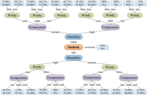
Table 5. A multi-valued training set containing 10 samples.

No.	Attributes				Class
	Outlook	Temperature	Humidity	Windy
$S1$	sunny	hot	normal	false	P
$S2$	rain	mild	high	true	N
$S3$	rain, sunny	cool, mild	normal	true	P
$S4$	overcast, rain	hot, cool	high, normal	false, true	P
$S5$	overcast	mild, hot	high, normal	false	P
$S6$	sunny, rain	hot, cool	high	true, false	N
$S7$	overcast, rain, sunny	cool, mild	normal	true	P
$S8$	rain, overcast	cool, mild, hot	normal, high	false	P
$S9$	sunny, rain	hot, cool, mild	normal	false, true	N
$S10$	rain, sunny, overcast	mild, cool, hot	normal, high	true, false	P

Source: The Authors.

Table 6. A new training sample set after quantity expanding.

No.	Attributes				Class
	Outlook	Temperature	Humidity	Windy
$S^{\prime }1$	sunny; sunny; sunny; sunny; sunny; sunny	hot; hot; hot; hot; hot; hot	normal; normal	false; false	P
$S^{\prime }2$	rain; rain; rain; rain; rain; rain	mild; mild; mild; mild; mild; mild	high; high	true; true	N
$S^{\prime }3$	rain, sunny; rain, sunny; rain, sunny	cool, mild; cool, mild; cool, mild	normal; normal	true; true	P
$S^{\prime }4$	overcast, rain; overcast, rain; overcast, rain	hot, cool; hot, cool; hot, cool	high, normal	false, true	P
$S^{\prime }5$	overcast; overcast; overcast; overcast; overcast; overcast	mild, hot; mild, hot; mild, hot	high, normal	false; false	P
$S^{\prime }6$	sunny, rain; sunny, rain; sunny, rain	hot, cool; hot, cool; hot, cool	high; high	true, false	N
$S^{\prime }7$	overcast, rain, sunny; overcast, rain, sunny	cool, mild; cool, mild; cool, mild	normal; normal;	true; true	P
$S^{\prime }8$	rain, overcast; rain, overcast; rain, overcast	cool, mild, hot; cool, mild, hot	normal, high	false; false	P
$S^{\prime }9$	sunny, overcast, rain; sunny, overcast, rain	hot, cool, mild; hot, cool, mild	normal; normal	false, true	N
$S^{\prime }10$	rain, sunny, overcast; rain, sunny, overcast	mild, cool, hot; mild, cool, hot	normal, high	true, false	P

Source: The Authors.

According to the steps to build a multi-valued DT, this subsection first performs the quantity matching in the original data set $S,$ and then calculates the least common multiple of the four attributes, then we can obtain their matching values when ${\theta }_1=6,$ ${\theta }_2=6,$ ${\theta }_3=2,$ and ${\theta }_4=2.$ Then, based on the result of quantity matching, the original data set $S$ is expanded to a new data set $S^{\prime }$ as shown in Table 6. It is found that the number and weights of attribute values in the same attribute are kept consistent. Further, we use the bifurcation criterion to select the optimal attributes and construct a DT.

In the following content, we only show the selection process of the first node. The calculation processes of other nodes are the same and the results are shown in Table 7.

Table 7. The bifurcation criterion value in the multi-valued preference environment.

Preference = “sunny”		Preference = “rain”
M (S′1, A2) =0.0222		M (S′2, A2) =0.1393
M (S′1, A3) =0.1776		M (S′2, A3) =0.1463
M (S′1, A4) =0.0143		M (S′2, A4) =0.0243
Select the attribute “A3”		Select the attribute “A3”
Pre = "sunny, high"	Pre = "sunny, normal"	Pre = "rain, high"	Pre = "rain, normal"
M (S′11, A2) = 0.1843	M (S′12, A2) = 0.0177	M (S′21, A2) = 0.1335	M (S′22, A2) = 0.0196
M (S′11, A4) = 0	M (S′12, A4) = 0.0008	M (S′21, A4) = 0.1860	M (S′22, A4) = 0.0218
Select the attribute “A2”, and the last attribute is “A4”		Select the attribute “A4”, and the last attribute is “A2”
Pre = “sunny, high, hot”	Pre = “sunny, normal, hot”	Pre = “rain, high, true”	Pre = “rain, normal, true”
“sunny, high, hot, true”	“sunny, normal, hot, true”	“rain, high, true, hot”	“rain, normal, true, hot”
“sunny, high, hot, false”	“sunny, normal, hot, false”	“rain, high, true, mild”	“rain, normal, true, mild”
Pre = “sunny, high, mild”	Pre= “sunny, normal, mild”	“rain, high, true, cool”	“rain, normal, true, cool”
“sunny, high, mild, true”	“sunny, normal, mild, true”	Pre = “rain, high, false”	Pre = “rain, normal, false”
“sunny, high, mild, false”	“sunny, normal, mild, false”	“rain, high, false, hot”	“rain, normal, false, hot”
Pre = “sunny, high, cool”	Pre = “sunny, normal, cool”	“rain, high, false, mild”	“rain, normal, false, mild”
“sunny, high, cool, true”	“sunny, normal, cool, true”	“rain, high, false, cool”	“rain, normal, false, cool”
“sunny, high, cool, false”	“sunny, normal, cool, false”

Source: The Authors.

First, we calculate the bifurcation information of the training data set $S$ and compute the bifurcation criterion of four attributes, and then select the attribute with the largest bifurcation criterion value as the root node. The main process is given as follows: $$\begin{array}{c}bi{f}_r(S^{\prime })=-\frac{3}{10}\hspace{0.17em}{\text{log}}_2\frac{3}{10}-\frac{7}{10}\hspace{0.17em}{\text{log}}_2\frac{7}{10}=0.8813\\ M(S^{\prime },A_1)=0.8813-[-\frac{19}{60}(\frac{13}{19}{\hspace{0.17em}\text{log}\hspace{0.17em}}_2\frac{13}{19}+\frac{6}{19}{\hspace{0.17em}\text{log}\hspace{0.17em}}_2\frac{6}{19})-\frac{8}{30}(1{\hspace{0.17em}\text{log}\hspace{0.17em}}_{2}1+0)-\frac{25}{60}(\frac{13}{25}{\hspace{0.17em}\text{log}\hspace{0.17em}}_2\frac{13}{25}+\frac{12}{25}{\hspace{0.17em}\text{log}\hspace{0.17em}}_2\frac{12}{25})]=0.1802\\ M(S^{\prime },A_2)=0.8813-[-\frac{7}{20}(\frac{16}{21}{\hspace{0.17em}\text{log}\hspace{0.17em}}_2\frac{16}{21}+\frac{10}{42}{\hspace{0.17em}\text{log}\hspace{0.17em}}_2\frac{10}{42})-\frac{7}{20}(\frac{13}{21}{\hspace{0.17em}\text{log}\hspace{0.17em}}_2\frac{13}{21}+\frac{8}{21}{\hspace{0.17em}\text{log}\hspace{0.17em}}_2\frac{8}{21})-\frac{3}{10}(\frac{13}{18}{\hspace{0.17em}\text{log}\hspace{0.17em}}_2\frac{13}{18}+\frac{15}{18}{\hspace{0.17em}\text{log}\hspace{0.17em}}_2\frac{15}{18})]=0.0129\\ M(S^{\prime },A_3)=0.8813-[-\frac{4}{10}(\frac{2}{4}{\hspace{0.17em}\text{log}\hspace{0.17em}}_2\frac{2}{4}+\frac{2}{4}{\hspace{0.17em}\text{log}\hspace{0.17em}}_2\frac{2}{4})-\frac{6}{10}(\frac{5}{6}{\hspace{0.17em}\text{log}\hspace{0.17em}}_2\frac{5}{6}+\frac{1}{6}{\hspace{0.17em}\text{log}\hspace{0.17em}}_2\frac{1}{6})]=0.0913\\ M(S^{\prime },A_4)=0.8813-[-\frac{5}{10}(\frac{3}{5}{\hspace{0.17em}\text{log}\hspace{0.17em}}_2\frac{3}{5}+\frac{2}{5}{\hspace{0.17em}\text{log}\hspace{0.17em}}_2\frac{2}{5})-\frac{5}{10}(\frac{4}{5}{\hspace{0.17em}\text{log}\hspace{0.17em}}_2\frac{4}{5}+\frac{1}{5}{\hspace{0.17em}\text{log}\hspace{0.17em}}_2\frac{1}{5})]=0.0349\end{array}$$

From the above calculation results, we can find that the attribute $A_1$ has the largest bifurcation criterion value, which is selected as the optimal attribute. Specifically, the attribute $A_1$ contains three branch nodes “sunny”, “overcast”, and “rain”, which divides the data set $S^{\prime }$ into three preferences $S_1^{‘},$ $S_2^{‘},$ and $S_3^{‘}.$ Furthermore, we calculate the classifications under the two branches of “sunny” and “rain”. The results are shown in Table 7.

In Table 7, the left part shows the classification process under the attribute value is “sunny”. The right part shows the classification process under the attribute value is “rain”. Obviously, under the two branches, the bifurcation criterion value of $A_3$ is greater than the values of $A_2$ and $A_4.$ Thus, the attribute $A_3$ is selected as the optimal node. Since the classification with respect to the attribute $A_3$ still contains $P$ and $N,$ then, $A_3$ is only used as a bifurcation node. The two preferences “high” and “normal” of attribute $A_3$ can divide the data set again. Thus, $S_1$ is divided into $S_{11}$ and $S_{12}.$ These two sets select the attributes from the remaining attributes $A_2$ and $A_4$ respectively as the next bifurcation node. Table 7 shows the more detailed results.

From the calculation results in Table 7, it can be seen that in $S_{11},$ the bifurcation criterion value of the attribute $A_2$ is greater than the value of $A_4.$ Thus, $A_2$ is selected as the bifurcation node in both sets. The last attribute $A_4$ is left as a stop node. Furthermore, in $S_{12},$ the bifurcation criterion value of the attribute $A_2$ is greater than the value of $A_4,$ and then $A_2$ is selected as the bifurcation node. Thus, only the last attribute $A_4$ is left as a stop node. Based on this, we temporarily get a DT that lacks classification results. Since the classification results also contain probabilities, we need to calculate them again.

Figure 1 is a probabilistic DT derived from the training data set. The ellipse represents the attribute of the bifurcation node, the better the classification performance is, the closer the attribute is to the root of the tree. The line denotes the division preference, and the rectangle shows the probability of the classification result. The upper and lower numbers represent the probabilities of the classification results respectively under the bifurcation, which are $P$ and $N.$ For example, when the preferences are “rain, high, false, mild”, we can find that the corresponding classification result is $P=100\%$ and $N=0\%.$ Obviously, $P$ is better than others under this branch. If preferences are “sunny, high, cool, false”, we can find that the corresponding classification result is $P=18.18\%$ and $N=81.82\%.$ Then, $N$ is better than others under this branch. If preferences are “sunny, high, hot, true”, we can find that the corresponding classification result is $P=55\%$ and $N=45\%.$ There is very little difference in the classification probabilities between $P$ and $N$ under this branch. Then, both the alternatives are equal.

As aforementioned, to develop a DT model in machine learning under the multi-valued preference environment, this section first proposes a weight and quantity matching method in the multi-valued preference environment. Then, the corresponding DT algorithm is proposed and applied to an illustrated example. In the next section, we develop a machine learning model in the probabilistic multi-valued preference environment.

4. The machine learning model in the probabilistic multi-valued preference environment

It is found that the probability of each preference is the same in the machine learning models under the multi-valued preference environment. However, in the real classification calculation process, the probability of each preference may be different. Therefore, in this section, we propose a machine learning model in the probabilistic multi-valued preference environment. First, we propose a DT algorithm under this environment in the following subsection.

4.1. The DT algorithm in the probabilistic multi-valued preference environment

The probabilistic multi-valued preference environment is a situation based on the expansion of the multi-valued preference. The training data set in the probabilistic multi-valued preference not only contains multi-valued preferences, but also each preference contains the different probability instead of the equal weight values.

In Section 3.1, to re-match the numbers and weights of the preferences under all the attributes, the original data $S$ in the multi-valued preference environment needs to be preprocessed. Then, we can ensure that each attribute is balanced during the calculation process. However, each preference in the probabilistic multi-valued environment contains a probability. It is unnecessary to preprocess the data in this environment and we can directly calculate the bifurcation criterion of each attribute. Based on this, we can select the optimal bifurcation node and bifurcation sub node. Additionally, in the probabilistic multi-valued preference environment, it is noted that since each preference contains the probability, the preference probability need to be added in the entire calculation process. Therefore, we can build a DT model in the probabilistic multi-valued preference environment, which is also a machine learning model. Some related notations used in this section are given in Table 8.

Table 8. Some main notations in the probabilistic multi-valued preference environment.

Notations	Introduction	Notations	Introduction
$T^{\prime }$	The new training data set after quantity matching	$\left|q_{iu}^c\right|$	The weight about the $u$ th preference of the sub node attribute $c$ in the $i$ th sample
$\left|T^{\prime }\right|$	The sample number of $T^{\prime }$	$\left|q_{\mathit{iuk}}^c\right|$	The weight about the $u$ th preference of the sub node attribute $c$ belongs to class $k$ in the $i$ th sample
$Q$	An attribute of $T^{\prime }$	$P_{iw}^Z{(b)}^{\prime }$	The preferences $q_{iw}$ of the root node attribute is under branch $Z,$ where there are $b$ samples with classification result $P$
$\left|C_k\right|$	The sample number of the class $C_k$	$P_{\mathit{icu}}^Z{(b)}^{\prime }$	The preference $q_{iu}$ of the $c$ th sub node is under branch $Z,$ where there are $b$ samples with classification result $P$
$\left|q_{iw}\right|$	The weight about the $w$ th preference of the root node attribute in the $i$ th sample	$N_{iw}^Z{(g)}^{\prime }$	The preference $q_{iw}$ of the root node attribute is under branch $Z,$ where there are $g$ samples with classification result $N$
$\left|q_{\mathit{iwk}}\right|$	The weight about the $w$ th preference in the root node attribute belongs to the class $k$ in the $i$ th sample	$N_{\mathit{icu}}^Z{(g)}^{\prime }$	The preference $q_{iu}$ of the $c$ th sub node is under branch $Z,$ where there are $g$ samples with classification result $N$

Source: The Authors.

Although this environment does not require preprocessing of the original training data set, we need to consider the probability contained in each preference. Then, we subdivide this modeling process into two steps, namely the selection of the root node and the other nodes.

The selection of the optimal root node is done individually, and each branch only considers a certain attribute. We calculate the bifurcation criterion of each attribute separately, and the attribute with the largest bifurcation criterion is the optimal one. There is only one optimal root node in a DT, while there may be multiple optimal sub nodes. The selection principle of all the sub nodes is the same. In this case, the sub node not only considers the current attribute and its belonging preference, but also considers all the previous nodes including the root node. Then, we can take the conditional probability in this environment as the probabilities of other sub nodes when the root node is known, and the corresponding probabilities are multiplied in the calculation process.

With respect to these principles, the calculation of the root node bifurcation criterion in the probabilistic multi-valued environment can be shown as (11) $$M{p}_r\left(T^{\prime },Q\right)=\mathit{Mpbi}{f}_r\left(T^{\prime }\right)-\mathit{Mpco}{n}_r\left(T^{\prime }/Q\right)$$(11)

Then, the bifurcation information entropy $\mathit{Mpbi}{f}_r(T^{\prime })$ of the root node is shown as (12) $$\mathit{Mpbi}{f}_r\left(T^{\prime }\right)=-{\sum }_{k=1}^K\frac{\left|C_k\right|}{\left|T^{\prime }\right|}{\hspace{0.17em}\text{log}\hspace{0.17em}}_2\frac{\left|C_k\right|}{\left|T^{\prime }\right|}\mathrm{ }\mathrm{ }$$(12)

Furthermore, the conditional information entropy of the root node is presented as follows: (13) $$\mathit{Mpco}{n}_r\left(T^{\prime }/Q\right)=-\sum _{i=1}^n\left[\sum _{w=1}^W\frac{\left|q_{iw}\right|}{\left|T^{\prime }\right|}\left(\sum _{k=1}^K\frac{\left|q_{\mathit{iwk}}\right|}{\left|q_{iw}\right|}{\hspace{0.17em}\text{log}\hspace{0.17em}}_2\frac{\left|q_{\mathit{iwk}}\right|}{\left|q_{iw}\right|}\mathrm{ }\mathrm{ }\right)\mathrm{ }\right]$$(13)

Similarly, the calculation of the sub node bifurcation criterion in the probabilistic multi-valued preference environment is summarized as follows: (14) $$M{p}_{\mathit{sub}}\left(T^{\prime },Q\right)=\mathit{Mpbi}{f}_{\mathit{sub}}\left(T^{\prime }\right)-\mathit{Mpco}{n}_{\mathit{sub}}\left(T^{\prime }/Q\right)$$(14)

Then, the bifurcation information entropy $\mathit{Mpbi}{f}_{\mathit{sub}}(T_w^{\prime })(w=1,2,\dots ,W)$ of the sub node is (15) $$\mathit{Mpbi}{f}_{\mathit{sub}}\left(T_w^{\prime }\right)=-\sum _{i=1}^n\sum _{k=1}^K\frac{\left|q_{\mathit{iwk}}\right|}{\left|q_{iw}\right|}{\hspace{0.17em}\text{log}\hspace{0.17em}}_2\frac{\left|q_{\mathit{iwk}}\right|}{\left|q_{iw}\right|}$$(15)

Moreover, the conditional information entropy of the sub node is presented as follows: (16) $$\mathit{Mpco}{n}_{\mathit{sub}}\left(T_{wc}^{\prime }/Q\right)=-\sum _{i=1}^n\frac{{\prod }_{u=1}^U(\left|q_{iu}^c\right|\cdot \left|q_{iw}\right|)}{\left|q_{iw}\right|}\cdot \left(\frac{\sum _{k=1}^K(\left|q_{iw}\right|\cdot {\prod }_{u=1}^U\left|q_{\mathit{iuk}}^c\right|)}{\left|q_{iw}\right|\cdot {\prod }_{u=1}^U\left|q_{iu}^c\right|}{\hspace{0.17em}\text{log}\hspace{0.17em}}_2\frac{\sum _{k=1}^K(\left|q_{iw}\right|\cdot {\prod }_{u=1}^U\left|q_{\mathit{iuk}}^c\right|)}{\left|q_{iw}\right|\cdot {\prod }_{u=1}^U\left|q_{iu}^c\right|}\right)$$(16)

Therefore, we can obtain the root node and sub node bifurcation criterion in the probabilistic multi-valued preference environment. Furthermore, we need to calculate the probability of each branch in the DT, and then obtain the probability $e_P^{\prime }$ that the classification result is $P$ by Eq. (17)(17) $$e_P^{\prime }=\frac{\sum _{b=1}^B(\left|P_{iw}^Z{(b)}^{\prime }\right|\cdot \prod _{u=1}^U\left|P_{\mathit{icu}}^Z{(b)}^{\prime }\right|)}{\sum _{b=1}^B(\left|P_{iw}^Z{(b)}^{\prime }\right|\cdot \prod _{u=1}^U\left|P_{\mathit{icu}}^Z{(b)}^{\prime }\right|)+\sum _{g=1}^G(\left|N_{iw}^Z{(g)}^{\prime }\right|\cdot \prod _{u=1}^U\left|N_{\mathit{icu}}^Z{(g)}^{\prime }\right|)}$$(17) . Similarly, we also can get $e_N^{\prime }.$ (17) $$e_P^{\prime }=\frac{\sum _{b=1}^B(\left|P_{iw}^Z{(b)}^{\prime }\right|\cdot \prod _{u=1}^U\left|P_{\mathit{icu}}^Z{(b)}^{\prime }\right|)}{\sum _{b=1}^B(\left|P_{iw}^Z{(b)}^{\prime }\right|\cdot \prod _{u=1}^U\left|P_{\mathit{icu}}^Z{(b)}^{\prime }\right|)+\sum _{g=1}^G(\left|N_{iw}^Z{(g)}^{\prime }\right|\cdot \prod _{u=1}^U\left|N_{\mathit{icu}}^Z{(g)}^{\prime }\right|)}$$(17)

Thus, we construct the DT model in machine learning under the probabilistic multi-valued preference environment, and the DT shows the probabilistic character. The above calculation process can be further shown by the following pseudo-code.

Table

Input: The training data set $T.$ Step 1: Treat each attribute $Q$ in the new training data set $T$′ as a node. Step 2: Traverse each preference $q$ of the current attribute and divide the data into different sub nodes by preference. Step 3: Use bifurcation criterion to determine the optimal preference for partitioning. Step 4: Consider the probability of each preference in the calculation process. Step 5: Traverse all the attributes by the second step, select the best attribute and the best preference of the attribute, and get the final sub node. Step 6: Continue to perform Steps 2-5 for all sub nodes, until each final sub node becomes a stop node, and obtain a DT. Step 7: Calculate the probability of the classification result under each branch in the DT.

Output: A probabilistic DT.

4.2. An illustrated example

In this section, to show the effectiveness and feasibility of the above algorithm in the probabilistic multi-valued preference environment, we give the detailed calculation process based on an illustrated example. To present the advantages, we follow the example in Subsection 3.2 and expand the data set to 60 samples which are shown in Table 9. We can find that the entire data set is divided into two parts, the first 50 samples are taken as the training data sets, and the last 10 samples are taken as the prediction data sets. In addition, the preference in each sample contains the probability and the sum of the preference probabilities is 1 in the same sample and attribute.

Table 9. The probabilistic multi-valued training set containing 60 samples.

NO.	Attributes				Class	NO.	Attributes				Class
	Outlook	Temperature	Humidity	Windy			Outlook	Temperature	Humidity	Windy
$T1$	sunny	hot	normal	false	P	$T31$	sunny, rain	hot, cool	normal	true	N
	1.0	1.0	1.0	1.0			0.33, 0.67	0.02, 0.98	1.0	1.0
$T2$	rain	mild	high	true	N	$T32$	overcast, rain	mild, cool	high, normal	true, false	P
	1.0	1.0	1.0	1.0			0.46, 0.54	0.19, 0.81	0.45, 0.55	0.2, 0.8
$T3$	sunny, rain	mild, cool	normal	true, false	P	$T33$	sunny	hot, cool	normal	true	P
	0.13, 0.87	0.28, 0.72	1.0	0.31, 0.69			1.0	0.17, 0.83	1.0	1.0
$T4$	overcast, rain	hot, cool	high, normal	true, false	P	$T34$	sunny, overcast, rain	mild	high	false	P
	0.75, 0.25	0.81, 0.19	0.88, 0.12	0.8, 0.2			0.2, 0.43, 0.37	1.0	1.0	1.0
$T5$	overcast	hot, mild	high, normal	false	P	$T35$	overcast	hot, cool	high	true, false	P
	1.0	0.43, 0.57	0.49, 0.51	1.0			1.0	0.03, 0.97	1.0	0.24, 0.76
$T6$	sunny, rain	hot, cool	high	true	N	$T36$	sunny, overcast, rain	hot, mild	normal	true	P
	0.9, 0.1	0.74, 0.26	1.0	1.0			0.19, 0.31, 0.5	0.06, 0.94	1.0	1.0
$T7$	sunny, overcast, rain	mild, cool	normal	true	P	$T37$	rain	cool	normal	false	N
	0.1, 0.78, 0.12	0.05, 0.95	1.0	1.0			1.0	1.0	1.0	1.0
$T8$	overcast, rain	hot, cool	high, normal	false	P	$T38$	sunny, rain	mild, cool	high	true, false	P
	0.31, 0.69	0.49, 0.51	0.17, 0.83	1.0			0.43, 0.57	0.49, 0.51	1.0	0.32, 0.68
$T9$	sunny, rain	mild	normal	true	N	$T39$	overcast	hot, mild	high, normal	false	P
	0.4, 0.6	1.0	1.0	1.0			1.0	0.59, 0.41	0.06, 0.94	1.0
$T10$	overcast, rain	hot, cool	high, normal	false	P	$T40$	rain	cool	normal	true	N
	0.55, 0.45	0.8, 0.2	0.21, 0.79	1.0			1.0	1.0	1.0	1.0
$T11$	sunny, rain	hot, mild	normal	true, false	N	$T41$	sunny, overcast, rain	mild, cool	high	true, false	P
	0.39, 0.61	0.73, 0.27	1.0	0.14, 0.86			0.14, 0.41, 0.45	0.07, 0.93	1.0	0.06, 0.94
$T12$	sunny, overcast, rain	mild, cool	high, normal	true	P	$T42$	overcast	hot mild	high, normal	false	P
	0.2, 0.23, 0.57	0.38, 0.62	0.05, 0.95	1.0			1.0	0.21, 0.79	0.09, 0.91	1.0
$T13$	overcast, rain	hot, cool	high	true, false	P	$T43$	sunny, overcast, rain	hot, cool	normal	true, false	P
	0.06, 0.94	0.26, 0.74	1.0	0.06, 0.94			0.28, 0.25, 0.47	0.03, 0.97	1.0	0.39, 0.61
$T14$	sunny, rain	mild	high, normal	false	P	$T44$	sunny	hot, mild	high	false	P
	0.27, 0.73	1.0	0.1, 0.9	1.0			1.0	0.16, 0.84	1.0	1.0
$T15$	overcast	hot, mild, cool	normal	true, false	P	$T45$	sunny, overcast, rain	cool	normal	true	P
	1.0	0.26, 0.14, 0.6	1.0	0.33, 0.67			0.25, 0.16, 0.59	1.0	1.0	1.0
$T16$	sunny, overcast, rain	hot, cool	high, normal	false	P	$T46$	rain	hot, cool	high, normal	true, false	N
	0.46, 0.19, 0.35	0.13, 0.87	0.33, 0.67	1.0			1.0	0.41, 0.59	0.08, 0.92	0.13, 0.87
$T17$	sunny, overcast	hot, mild, cool	high	true, false	P	$T47$	sunny, overcast	hot, mild	high, normal	true, false	P
	0.77, 0.23	0.1, 0.26, 0.64	1.0	0.02, 0.98			0.49, 0.51	0.06, 0.94	0.07, 0.93	0.4, 0.6
$T18$	rain	mild	high, normal	true, false	N	$T48$	overcast, rain	mild	high	true	P
	1.0	1.0	0.08, 0.92	0.29, 0.71			0.42, 0.58	1.0	1.0	1.0
$T19$	sunny, rain	hot, mild, cool	normal	true	N	$T49$	sunny, overcast	hot, cool	normal	true, false	P
	0.43, 0.57	0.09, 0.33, 0.58	1.0	1.0			0.3, 0.7	0.42, 0.58	1.0	0.15, 0.85
$T20$	sunny, overcast	hot	high, normal	true, false	P	$T50$	sunny, rain	mild	high, normal	false	N
	0.78, 0.22	1.0	0.18, 0.82	0.01, 0.99			0.24, 0.76	1.0	0.35, 0.65	1.0
$T21$	sunny, overcast, rain	mild, cool,	high	false	P	$T51$	sunny, rain	cool, hot	high, normal	true	P 50.05% N 49.95%
	0.16, 0.23, 0.61	0.08, 0.92,	1.0	1.0			0.19, 0.81	0.29, 0.71	0.06, 0.94	1.0
$T22$	overcast	hot	normal	true, false	P	$T52$	overcast, sunny, rain	hot, mild	normal	true, false	P 48.62% N 51.38%
	1.0	1.0	1.0	0.28, 0.72			0.18, 0.77,0.05	0.27, 0.73	1.0	0.91, 0.09
$T23$	sunny, rain	hot, mild, cool	high, normal	true, false	N	$T53$	overcast, rain	cool	high, normal	false	P 91.68% N 8.32%
	0.49, 0.51	0.05, 0.19, 0.76	0.07, 0.93	0.39, 0.61			0.54, 0.46	1.0	0.72, 0.28	1.0
$T24$	overcast, rain	mild	normal	false	P	$T54$	sunny, overcast	mild, cool, hot	normal	true	P 96.8% N 3.2%
	0.43 0.57	1.0	1.0	1.0			0.09, 0.91	0.10, 0.17, 0.73	1.0	1.0
$T25$	rain	hot, mild, cool	normal	true	N	$T55$	rain, sunny, overcast	hot, cool	high	true, false	P 74.91% N 25.09%
	1.0	0.08, 0.05, 0.87	1.0	1.0			0.39, 0.48, 0.13	0.39, 0.61	1.0	0.95, 0.05
$T26$	sunny, overcast, rain	hot, cool	high, normal	true, false	P	$T56$	sunny	hot, mild, cool	normal, high	false	P 85% N 15%
	0.46, 0.4, 0.14	0.1, 0.9	0.16, 0.84	0.34, 0.66			1.0	0.23, 0.42, 0.35	0.83, 0.17	1.0
$T27$	sunny	hot, mild, cool	high	true, false	P	$T57$	overcast, sunny, rain	mild	normal	true, false	P 68.41% N 31.59%
	1.0	0.02, 0.19, 0.79	1.0	0.17, 0.83			0.03, 0.71, 0.26	1.0	1.0	0.40, 0.60
$T28$	overcast	cool	normal	false	P	$T58$	rain, overcast	mild, hot	high	true	P 72.13% N 27.87%
	1.0	1.0	1.0	1.0			0.86, 0.14	0.73, 0.27	1.0	1.0
$T29$	sunny, overcast, rain	hot, mild,	high	true, false	P	$T59$	sunny, rain	hot, cool	high, normal	false	P 72.18% N 27.82%
	0.12, 0.29, 0.59	0.7, 0.3,	1.0	0.02, 0.98			0.36, 0.64	0.88, 0.12	0.52, 0.48	1.0
$T30$	overcast, rain	mild, cool	high, normal	false	P	$T60$	rain	cool, mild	normal, high	true, false	P 68.11% N 31.89%
	0.21, 0.79	0.67, 0.33	0.44, 0.56	1.0			1.0	0.69,0.31	0.71,0.29	0.30,0.70

Source: The Authors.

In this example, we only show the calculation process of the root node selection. Similarly, the selection of other sub nodes can be calculated. The calculation results are shown in Table 10. $$\begin{array}{c}bif(T^{\prime })=-\frac{27}{50}\hspace{0.17em}{\text{log}}_2\frac{27}{50}-\frac{13}{50}\hspace{0.17em}{\text{log}}_2\frac{13}{50}=0.9853\\ M(T^{\prime },A_1)=0.9853-[-\frac{12.91}{50}(\frac{9.73}{12.91}{\hspace{0.17em}\text{log}\hspace{0.17em}}_2\frac{9.73}{12.91}+\frac{3.18}{12.91}{\hspace{0.17em}\text{log}\hspace{0.17em}}_2\frac{3.18}{12.91})-\frac{21.56}{50}(\frac{11.74}{21.56}{\hspace{0.17em}\text{log}\hspace{0.17em}}_2\frac{11.74}{21.56}+\frac{9.82}{21.56}{\hspace{0.17em}\text{log}\hspace{0.17em}}_2\frac{9.82}{21.56})]=0.3486\\ M(T^{\prime },A_2)=0.9853-[-\frac{10.95}{50}(\frac{8.83}{10.95}{\hspace{0.17em}\text{log}\hspace{0.17em}}_2\frac{9.83}{10.95}+\frac{2.12}{10.95}{\hspace{0.17em}\text{log}\hspace{0.17em}}_2\frac{2.12}{10.95})-\frac{16.43}{50}(\frac{11.59}{16.43}{\hspace{0.17em}\text{log}\hspace{0.17em}}_2\frac{11.59}{16.43}+\frac{4.84}{16.43}{\hspace{0.17em}\text{log}\hspace{0.17em}}_2\frac{4.84}{16.43})\\ -\frac{22.62}{50}(\frac{16.58}{22.62}{\hspace{0.17em}\text{log}\hspace{0.17em}}_2\frac{16.58}{22.62}+\frac{6.04}{22.62}{\hspace{0.17em}\text{log}\hspace{0.17em}}_2\frac{6.04}{22.62})]=0.1639\\ M(T^{\prime },A_3)=0.9853-[-\frac{17.26}{50}(\frac{14.68}{17.26}{\hspace{0.17em}\text{log}\hspace{0.17em}}_2\frac{14.68}{17.26}+\frac{3.58}{17.26}{\hspace{0.17em}\text{log}\hspace{0.17em}}_2\frac{3.58}{17.26})-\frac{32.74}{10}(\frac{22.32}{32.74}{\hspace{0.17em}\text{log}\hspace{0.17em}}_2\frac{22.32}{32.74}+\frac{9.42}{32.74}{\hspace{0.17em}\text{log}\hspace{0.17em}}_2\frac{9.42}{32.74})]=0.1689\\ M(T^{\prime },A_4)=0.9853-[-\frac{18.05}{50}(\frac{10.1}{18.05}{\hspace{0.17em}\text{log}\hspace{0.17em}}_2\frac{10.1}{18.05}+\frac{7.95}{18.05}{\hspace{0.17em}\text{log}\hspace{0.17em}}_2\frac{7.95}{18.05})-\frac{31.95}{50}(\frac{26.9}{31.95}{\hspace{0.17em}\text{log}\hspace{0.17em}}_2\frac{26.9}{31.95}+\frac{5.05}{31.95}{\hspace{0.17em}\text{log}\hspace{0.17em}}_2\frac{5.05}{31.95})]=0.2257\end{array}$$

Table 10. The bifurcation criterion value about sub nodes in the probabilistic multi-valued environment.

Preference = “sunny”		Preference = “rain”
M (T′1, A2) =0.0439		M (T′3, A2) =0.0010
M (T′1, A3) =0.0461		M (T′3, A3) =0.0300
M (T′1, A4) =0.1767		M (T′3, A4) =0.0590
Select the attribute “A4”		Select the attribute “A4”
Pre = “sunny, true”	Pre = “sunny, false”	Pre = “rain, true”	Pre= “rain, false”
M (T′11, A2) = 0.0825	M (T′12, A2) = 0.0177	M (T′31, A2) = 0.0036	M (T′32, A2) = 0.0016
M (T′11, A3) = 0.0971	M (T′12, A4) = 0.0008	M (T′31, A3) = 0.1470	M (T′32, A3) = 0.0192
Select the attribute “A3”, and the last attribute is “A2”		Select the attribute “A3”, and the last attribute is “A2”
Pre = “sunny, true, high”	Pre= “sunny, true, normal”	Pre = “rain, true, high”	Pre = “rain, false, high”
“sunny, true, high, hot”	“sunny, true, normal, hot”	“rain, true, high, hot”	“rain, false, high, hot”
“sunny, true, high, mild”	“sunny, true, normal, mild”	“rain, true, high, hot”	“rain, false, high, mild”
“sunny, true, high, cool”	“sunny, true, normal, cool”	“rain, true, high, hot”	“rain, false, high, cool”
Pre = “sunny, false, high”		Pre = “rain, true, normal”	Pre = “rain, false, normal”
		“rain, true, normal, hot”	“rain, false, normal, hot”
		“rain, true, normal, mild”	“rain, false, normal, mild”
		“rain, true, normal, cool”	“rain, false, normal, cool”

Source: The Authors.

The above calculation shows the selection process of the root node. From the results, we can find that the attribute $A_1$ has the largest bifurcation criterion value, and then the attribute $A_1$ can be selected as the optimal attribute. Specifically, the three preferences “sunny”, “overcast”, and “rain” in the attribute $A_1$ divided data set $T^{\prime }$ into three kinds of preferences $T_1^{\prime },$ $T_2^{\prime },$ and $T_3^{\prime }.$

When the preference contained in the branch is “overcast”, we can find that all the classification results are unique and the category is $P.$ In this case, there is no need to further divide this node, and then the classification process is end.

Then, we calculate the bifurcation criterion of other attributes in the two kinds of preferences $T_1^{\prime },$ and $T_3^{\prime },$ namely “sunny” and “rain”, to find all the sub nodes. This calculation process involves more multi-attribute bifurcation criterion. The bifurcation criterion values and node selection results are given in Table 10. Then, we can find that the attribute selection order is $A_1,$ $A_4,$ $A_3,$ and $A_2.$ Based on this, we can get a DT in machine learning. At last, we use Eq. (17)(17) $$e_P^{\prime }=\frac{\sum _{b=1}^B(\left|P_{iw}^Z{(b)}^{\prime }\right|\cdot \prod _{u=1}^U\left|P_{\mathit{icu}}^Z{(b)}^{\prime }\right|)}{\sum _{b=1}^B(\left|P_{iw}^Z{(b)}^{\prime }\right|\cdot \prod _{u=1}^U\left|P_{\mathit{icu}}^Z{(b)}^{\prime }\right|)+\sum _{g=1}^G(\left|N_{iw}^Z{(g)}^{\prime }\right|\cdot \prod _{u=1}^U\left|N_{\mathit{icu}}^Z{(g)}^{\prime }\right|)}$$(17) to calculate the probability of each branch in the tree and get a probabilistic DT, which are shown in Figure 2.

Figure 2. The DT based on the information gain and the data set ${\mathit{T}}^{\prime }.$

Source: The Authors.

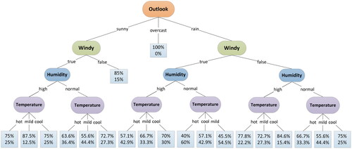
Based on Figure 2, we can obtain the probabilities of all the branches in the DT and their corresponding classification results. As shown in Figure 2, the ellipse represents the bifurcation node, the line represents the division preference, and the rectangle denotes the probability of the classification result. The upper and lower numbers in the rectangle refer to the probabilities of the classification results, which are $P$ and $N$ respectively. According to this, we can further obtain the classification results of the prediction data set. Moreover, Figure 2 shows all the probabilities of the classification results for $P$ and $N.$

As aforementioned, in this section, we propose a DT model in machine learning under the probabilistic multi-valued preference environment. In addition, we apply them to an illustrated example which reflects their feasibility and effectiveness.

5. Conclusions

In the classification process, the data are often not unique, there may be multiple values and probabilities, and then it is meaningful to develop an appropriate method to make a classification decision in this situation. To do this, this paper has given the multi-valued preference environment and probabilistic multi-valued preference environment, and then constructed two optimization machine learning methods based on the new DT models. First, in the multi-valued preference environment, a training data set with matching quantity and weight has been obtained through data preprocessing, and a DT model in the multi-valued preference environment has been proposed by using the entropy to generate several branches and probabilistic classifications. Then, according to the different probabilities, we have developed a DT model in the probabilistic multi-valued preference environment, and the branches and their corresponding probabilities have been similarly generated. Meanwhile, we have given two illustrated examples to show the calculation process and proved the feasibility of the proposed machine learning methods. Therefore, there are three contributions of this paper: (1) This paper has proposed a data preprocessing method to match the weights and numbers in the multi-valued preference environment; (2) This paper has developed a machine learning method and a DT algorithm in the multi-valued preference environment to obtain the corresponding probability classification; (3) This paper has constructed a machine learning method and a DT algorithm in the probabilistic multi-valued preference environment, and the corresponding probability classification has been obtained.

The machine learning methods and the DT algorithms in the multi-valued preference and probabilistic multi-valued preference environments have been proposed in this paper. These can show the practical significance and provide decision makers with reasonable classification decision suggestions. However, these methods also have some limitations in data preprocessing. For example, they are only suitable for the small samples. These limitations are also the focus of our future research.

Disclosure statement

No potential conflict of interest was reported by the authors.

Additional information

Funding

This work was supported by Natural Science Foundation of China (Nos. 72071176 and 71840001).

References

- Barlow, H. B. (1989). Unsupervised learning. Neural Computation, 1(3), 295–311. https://doi.org/10.1162/neco.1989.1.3.295
- Bhargava, D. N., Sharma, G., Bhargava, R., & Mathuria, M. (2013). Decision tree analysis on j48 algorithm for data mining. Proceedings of International Journal of Advanced Research in Computer Science and Software Engineering, 3(6), 22–45.
- Blum, A. L., & Langley, P. (1997). Selection of relevant features and examples in machine learning. Artificial Intelligence, 97(1–2), 245–271. https://doi.org/10.1016/S0004-3702(97)00063-5
- Capó, M., Pérez, A., & Lozano, J. A. (2020). An efficient K-means clustering algorithm for tall data. Data Mining and Knowledge Discovery, 34(3), 776–811. https://doi.org/10.1007/s10618-020-00678-9
- Chen, B., Gu, W., & Hu, J. (2010). An improved multi-label classification method and its application to functional genomics. International Journal of Computational Biology and Drug Design, 3(2), 133–145. https://doi.org/10.1504/IJCBDD.2010.035239
- Chen, Y.-L., Hsu, C.-L., & Chou, S.-C. (2003). Construction a multi-valued and multi-label decision tree. Expert Systems with Applications, 25(2), 199–209. https://doi.org/10.1016/S0957-4174(03)00047-2
- Cheng, J. (2014). A study of improving the performance of mining multi-valued and multi-labeled data. Informatica, 25(1), 95–111.
- Chou, S., & Hsu, C. L. (2005). MMDT: A multi-valued and multi-labeled decision tree classifier for data mining. Expert Systems with Applications, 28(4), 799–812. https://doi.org/10.1016/j.eswa.2004.12.035
- Clarke, K. R. (1993). Non‐parametric multivariate analyses of changes in community structure. Austral Ecology, 18(1), 117–143. https://doi.org/10.1111/j.1442-9993.1993.tb00438.x
- Crawford, S. L. (1989). Extension to the CART algorithm. International Journal of Man-Machine Studies, 31(2), 197–217. https://doi.org/10.1016/0020-7373(89)90027-8
- Figueiredo, M. A. T. (2003). Adaptive sparseness for supervised learning. IEEE Transactions on Pattern Analysis and Machine Intelligence, 25(9), 1150–1159. https://doi.org/10.1109/TPAMI.2003.1227989
- Galton, F. (1889). Co-relations and their measurement, chiefly from anthropometric data. Proceedings of the Royal Society of London, 45, 135–145.
- Gerfo, L. L., Rosasco, L., Odone, F., Vito, E. D., & Verri, A. (2008). Spectral Algorithms for Supervised Learning. Neural Computation, 20(7), 1873–1897. https://doi.org/10.1162/neco.2008.05-07-517
- Goldsmith, J. (2001). Unsupervised learning of the morphology of a natural language. Computational Linguistics, 27(2), 153–198. https://doi.org/10.1162/089120101750300490
- Han, J. W., & Micheline, K. (2006). Data mining: Concepts and techniques. In Data mining concepts models methods & algorithms (2nd ed., Vol. 5, pp. 1–18). Morgan Kaufmann.
- Han, Q. Q., Liu, J. M., Shen, Z. W., Liu, J. W., & Gong, F. K. (2020). Vector partitioning quantization utilizing K-means clustering for physical layer secret key generation. Information Sciences, 512, 137–160. https://doi.org/10.1016/j.ins.2019.09.076
- Hardikar, S., Shrivastava, A., & Choudary, V. (2012). Comparison between ID3 and C4.5. International Journal of Computer Science, 2(7), 34–39.
- Hsu, C. L. (2021). A multi-valued and sequential-labeled decision tree method for recommending sequential patterns in cold-start situations. Applied Intelligence, 51(1), 506–526. https://doi.org/10.1007/s10489-020-01806-0
- Hunt, E. (1965). Selection and reception conditions in grammar and concept learning. Journal of Verbal Learning and Verbal Behavior, 4(3), 211–215. https://doi.org/10.1016/S0022-5371(65)80022-6
- Kruppa, J., Schwarz, A., Arminger, G., & Ziegler, A. (2013). Consumer credit risk: Individual probability estimates using machine learning. Expert Systems with Applications, 40(13), 5125–5131. https://doi.org/10.1016/j.eswa.2013.03.019
- Lee, T. R., Wood, W. T., & Phrampus, B. J. (2019). A machine learning (KNN) approach to predicting global seafloor total organic carbon. Global Biogeochemical Cycles, 33(1), 37–46. https://doi.org/10.1029/2018GB005992
- Mantas, C. J., Castellano, J. G., Moral, G. S., & Abellán, J. (2019). A comparison of random forest based on algorithms: Random credal random forest versus oblique random forest. Soft Computing, 23(21), 10739–10754. https://doi.org/10.1007/s00500-018-3628-5
- Miao, D. Q., & Wang, J. (1997). Rough sets based on approach for multivariate decision tree construction. Journal of Software, 8(6), 425–431.
- Narasimha, P. L. V., & Naidu, M. M. (2014). CC-SLIQ: Performance enhancement with 2k split points in SLIQ decision tree algorithm. IAENG International Journal of Computer Science, 41(3), 163–173.
- Pal, M., & Mather, P. M. (2003). An assessment of the effectiveness of decision tree methods for land cover classification. Remote Sensing of Environment, 86(4), 554–565. https://doi.org/10.1016/S0034-4257(03)00132-9
- Pal, R., Kupka, K., Aneja, A. P., & Militky, J. (2016). Business health characterization: A hybrid regression and support vector machine analysis. Expert Systems with Applications, 49, 48–59. https://doi.org/10.1016/j.eswa.2015.11.027
- Polat, K., & Güneş, S. (2007). Classification of epileptiform EEG using a hybrid system based on decision tree classifier and fast Fourier transform. Applied Mathematics and Computation, 187(2), 1017–1026. https://doi.org/10.1016/j.amc.2006.09.022
- Qayyum, A., Usama, M., Qadir, J., & Al-Fuqaha, A. (2020). Securing future autonomous & connected vehicles: Challenges posed by adversarial machine learning and the way forward. IEEE Communications Surveys & Tutorials, 22(2), 998–1026.
- Quinlan, J. R. (1986). Induction of decision trees. Machine Learning, 1(1), 81–106. https://doi.org/10.1007/BF00116251
- Quinlan, J. R. (1987). Simplifying decision trees. International Journal of Man-Machine Studies, 27(3), 221–234. https://doi.org/10.1016/S0020-7373(87)80053-6
- Quinlan, J. R. (1996). Improved use of continuous attributes in C4.5. Journal of Artificial Intelligence Research, 4(1), 77–90. https://doi.org/10.1613/jair.279
- Ruggieri, S. (2002). Efficient C4.5 classification algorithm. IEEE Transactions on Knowledge and Data Engineering, 14(2), 438–444. https://doi.org/10.1109/69.991727
- Rutkowski, L., Jaworski, M., Pietruczuk, L., & Duda, P. (2014). The CART decision tree for mining data streams. Information Sciences, 266(1), 1–15. https://doi.org/10.1016/j.ins.2013.12.060
- Santhosh, K. (2013). Modified C4.5 algorithm with improved information entropy. International Journal of Engineering Research & Technology, 2(14), 485–512.
- Santini, S., & Jain, R. (1999). Similarity measures. IEEE Transactions on Pattern Analysis & Machine Intelligence, 21(9), 871–883.
- Sun, Z. L., Choi, T. M., Au, K. F., & Yu, Y. (2008). Sales forecasting using extreme learning machine with applications in fashion retailing. Decision Support Systems, 46(1), 411–419. https://doi.org/10.1016/j.dss.2008.07.009
- Tsoumakas, G. (2019). A survey of machine learning techniques for food sales prediction. Artificial Intelligence Review, 52(1), 441–447. https://doi.org/10.1007/s10462-018-9637-z
- Tversky, A. (1977). Features of similarity. Psychological Review, 84(4), 327–352. https://doi.org/10.1037/0033-295X.84.4.327
- Utkin, L. V. (2019). An imprecise extension of SVM-based machine learning models. Neurocomputing, 331, 18–32.
- Wong, W. K., & Guo, Z. X. (2010). A hybrid intelligent model for medium-term sales forecasting in fashion retail supply chains using extreme learning machine and harmony search algorithm. International Journal of Production Economics, 128(2), 614–624. https://doi.org/10.1016/j.ijpe.2010.07.008
- Yi, W., Lu, M., & Liu, Z. (2011). Multi-valued attribute and multi-labeled data decision tree algorithm. Pattern Recognition & Artificial Intelligence, 2(2), 67–74.
- Yuan, R. X., Li, Z., Guan, X. H., & Xu, L. (2010). An SVM-based machine learning method for accurate internet traffic classification. Information Systems Frontiers, 12(2), 149–156. https://doi.org/10.1007/s10796-008-9131-2
- Zhang, M. L., & Zhou, Z. H. (2007). ML-KNN: A lazy learning approach to multi-label learning. Pattern Recognition, 40(7), 2038–2048. https://doi.org/10.1016/j.patcog.2006.12.019
- Zhao, R., & Li, H. (2007). Algorithm of multi-valued attribute and multi-labeled data decision tree. Computer Engineering, 33(13), 87–89.