Combined probabilistic linguistic term set and ELECTRE II method for solving a venture capital project evaluation problem

Abstract

Multiple criteria decision making (MCDM) frameworks assist people in assessing alternatives and making reasonable decisions, with the ELECTRE II MCDM method in particular being widely applied to many diverse fields. As it is not always possible to assess qualitative attributes or accurately evaluate alternatives using precise values, this paper proposes a new approach that combines the ELECTRE II method with probabilistic linguistic term sets (PLTS) to allow decision makers to state their qualitative preferences using corresponding probabilities. To demonstrate the viability of the PTLS-ELECTRE II method and assess its practicability, the proposed method was applied to a typical MCDM venture capital project evaluation problem, for which a comprehensive venture capital project evaluation index system was constructed that included multiple qualitative and quantitative indicators, such as industry background, marketing, product technology, team management and financial data. The reasonable evaluation sequence of alternatives was then determined using the PTLS-ELECTRE II method which can provide more accurate MCDM decisions.

Keywords:

• Multiple criteria decision-making
• ELECTRE II method
• Probabilistic linguistic term set
• Venture capital project evaluation

JEL CODES:

• C44; D81; G24

1. Introduction

When people make a decision, they generally have to consider multiple criteria, which are known as multiple criteria decision making (MCDM) problems. MCDM decision-making research on relevant theories and solutions has been an important part of operational research and management (Govindan & Jepsen, 2016). A large number of MCDM methods have been developed, such as the Technique of Order Preference Similarity to the Ideal Solution (TOPSIS), ELimination Et Choix Traduisant la REalité (ELECTRE), the Analytic Hierarchy Process (AHP), the analytic network process (ANP), and the Preference Ranking Organization Method for Enrichment of Evaluations (PROMETHEE).

MCDM methods have been widely applied in many different fields. To systematically review the range of MCDM techniques and methodologies, Mardani et al. (2015) reviewed 393 articles and grouped them into over 15 fields: energy, environment and sustainability, supply chain management, materials, quality management, GIS, construction and project management, safety and risk management, manufacturing systems, technology management, operation research and soft computing, strategic management, knowledge management, production management, and tourism management.

The ELECTRE method was first proposed by Benayoun et al. (1966), and Roy (1968) described it in detail in a journal article, naming it ELECTRE I. Over the following 20 years, ELECTRE methods received widespread attention and were being continually developed and improved. ELECTRE II in particular was designed for ranking problems and particularly accounts for outranking degrees of actions (Roy & Bertier, 1973) by constructing different concordance and discordance sets based on the degree to which one alternative is superior to another with respect to a specific criterion. By assigning weights, several concordance and discordance outranking relations levels can be aggregated to support the ranking computations (Liao et al., 2018). Because ELECTRE II can successfully rank alternatives, it has been widely used to solve multiple criteria decision making problems. For example, Gershon et al. (1982), researcher in natural resources and environmental management, studied and compared three MCDM methods including ELECTRE II for watershed planning. Elshorbagy (2006) used ELECTRE II and AVF for a multi-criteria watershed management decision problem that had seven evaluation indicators. Coronado et al. (2011) used EV, WS, ELECTRE II and REG methods to evaluate construction and demolition waste management in northern Spain and assess the sensitivity of the results. Alexopoulos et al. (2012) established an index system that had nine attributes and used the ELECTRE II method to rank enterprise management corporate strategies in the publishing industry.

Because of the uncertainties and limitations of human judgement, it is often difficult to obtain accurate evaluation information. ELECTRE II methods have also been widely applied in fuzzy environments, with many fuzzy escalated approaches developed (Ghorabaee et al., 2017). For example, Chen and Xu (2015) proposed a method of combining hesitant fuzzy sets and ELECTRE II. By defining the concepts of hesitant fuzzy concordance and discordance sets, and by constructing strong and weak ranking relationships, rankings are determined to deal with different opinions of multi-criteria decision-making members. Ferreira et al. (2016) proposed a fuzzy decision-making method combining the elements of fuzzy-ELECTRE and fuzzy-TOPSIS to establish a new ranking procedure and obtained good results in experiments. Liang et al. (2019) used the picture fuzzy number to express the evaluation information of the green mine, and proposed a novel multi-criteria decision-making method, which integrates the TODIM method with the elimination and the ELECTRE method in the picture fuzzy environment. Combining bipolar fuzzy set with ELECTRE II, Shumaiza et al. (2019) proposed a new multi-criteria decision model. By using optimisation techniques based on the maximum deviation method, the standard normalised weights that may not be fully understood by the decision maker can be calculated. Chen (2020) developed an extended ELECTRE method based on the Chebyshev distance metric to conduct multi-criteria decision analysis involving PF information to determine the partial and complete ranking of candidate alternatives, and conducted a practical application of comparative analysis to test Effectiveness. Niu et al. (2020) proposed a fuzzy MCDM technology based on interval value hesitation elimination and selection to represent reality, and took into account the uncertainty and ambiguity of information, and ranked renewable energy alternatives. Akram et al. (2020) proposed a hesitant fuzzy N-soft ELECTRE-II method. First, the concept of the notion of hesitant fuzzy N-soft concordance and discordance sets was described, and then the strong and weak sorting relationship was constructed for sorting.

In reality, decision makers usually tend to use words to express their assessment information. The linguistic variables concept was first proposed by Zadeh (1975); decision makers could be able to give their evaluation values more naturally. With the application in decision making (Herrera & Herrera-Viedma, 2000), quality assessment (Celotto et al., 2015) and many other fields, the linguist decision making has made great progress and is developing and improving continuously. Considering decision makers often showed hesitance between the possible linguistic choices, Rodriguez et al. (2012) proposed hesitant fuzzy linguistic term set (HFLTS), which allowed decision makers to express their preferences using more than one word. Liao et al. (2018) used HFLTS to extend the ELECTRE II method, and applied the new method to solve the selection of the well-performed maintenance servicing. Liu et al. (2020) proposed the improved ELECTRE II method with unknown weight information under the double hierarchy hesitant fuzzy linguistic term set to deal with a selection of public service outsourcer. However, in most HFLTS studies, each linguistic term has been given equal importance or weight, which is obviously not in accordance with reality. Therefore, to overcome this HFLTS disadvantage, Pang et al. (2016) proposed the probabilistic linguistic term set (PLTS), which assigned a probability to each linguistic term. The PLTS enriched the methods available for decision makers to give their preference information and enhanced their ability to express uncertain information. Since the PLTS was proposed, it has also been combined with ELECTRE method to solve MCDM problems. Liao et al. (2019) proposed novel PLTS operations and implemented the new ELECTRE III method to solve nurse-patient relationship problems. Mao et al. (2019) proposed a new method for solving MAGDM problems with PLTSs, which generate the ranking order of alternatives by integrating ELECTRE and TOPSIS.

Venture capital was defined by the Organization for Economic Cooperation and Development (OECD) as equity capital investment into start-ups or small businesses that have great competitive potential. Venture capital often follows a rigorous decision-making process, and Batterson (1986) points out that a well-regulated investment decision-making process can reduce the risk of failing to invest in a start-up. The venture capital project evaluation is a typical multi-attribute group decision-making problem. To solve the investment decision problem, scholars have done a lot of research related to the index system of venture capital project selection. The index system usually covers quantitative financial indicators which can be used to assess a company's operating profitability, development ability, debt paying ability and risk situation, as well as some important and often uncertain qualitative attributes, such as the management capabilities, technical product feasibility and uniqueness marketing abilities and the industry situation also need to be assessed. Cheng et al. (2017) proposed that an important issue in the investment decision is the expression of assessment information, and the venture capitalist are more likely to use fuzzy expressions in the evaluation of venture capital. Therefore, using the PLTSs to describe these qualitative attributes is more suitable and could better reflect the investors’ decision preferences.

This paper makes the following contributions:

1. A method combining PLTS and ELECTRE II is proposed to solve the multiple criteria decision making problems.

2. In the process of constructing the discordance index, this paper uses the novel score function called ScoreC-PLTS proposed by Lin et al. (2021). Compared with the original PLTS distance measurement method that needs to insert linguistic items for PLTS comparison, ScoreC-PLTS does not need to extend the shorter PLTS. This avoids the distortion of the original evaluation information and makes the construction of the PLTS discordance index more reasonable.

3. A comprehensive venture capital project evaluation index system is constructed that includes both quantitative and qualitative attributes.

4. We use the PLTS-ELECTRE II method to select the most appropriate projects for venture capital investment and provide an illustrative example.

The remainder of this paper is organised as follows. Section 2 introduces the PTLS and ELECTRE II concepts, Section 3 details the probabilistic linguistic concordance and discordance indices and the PLTSs-ELECTRE II method framework, Section 4 constructs the venture capital project qualitative and quantitative evaluation index, Section 5 gives a case study of venture capital project selection to demonstrate the proposed method, and conclusion is given in Section 6.

2. Relevant PLTS and ELECTRE II theories

2.1. PLTS

2.1.1. The LTS and the HFLTS

Decision makers could use LTSs to express their opinions on the considered objects. The additive LTS, which is finite and totally ordered, has been the most widely used LTS, and is defined as follows:$S=\{S_t\mid t=-\tau ,\dots ,-1,0,1,\dots ,\tau \},$ where $S_t$ is a possible value for a linguistic variable, $\mathrm{\tau }$ is a positive integer, and $S_{-\tau }$ and $S_{\tau }$ are the lower and upper limits of the linguistic terms.

As decision makers may hesitate between several possible values, Rodríguez et al. (2012) introduced the hesitant fuzzy linguistic term set (HFLTS):

Definition 1

(Rodríguez et al., 2012) Let $S=\{S_{\alpha }\mid \alpha =-\tau ,\dots ,-1,0,1,\dots ,\tau \}$ be an LTS, then the HFLTS is an ordered finite subset of the consecutive linguistic terms for $S.$

Example 1.

When $\tau =3,$ a LTS can be taken as:$S=\left\{s_{-3}=\mathit{very}\mathrm{}\mathit{low},s_{-2}=\mathit{low},s_{-1}=\mathit{slightly}\mathrm{}\mathit{low},s_0=\mathit{fair},s_1=\mathit{slightly}\mathrm{}\mathit{high},s_2=\mathit{high},\mathrm{}{s}_3=\mathit{very}\mathrm{}\mathit{high}\right\}.$Suppose that the linguistic expression opinions given by a decision maker are ‘at least low’ and ‘at least fair but no more than high’, then two HFLTSs are obtained： $$h_s\left(x_1\right)=\left\{s_{-2},s_{-1},s_0,s_1,s_2,s_3\right\}$$ $$h_s\left(x_1\right)=\left\{s_0,s_1,s_2\right\}$$

2.1.2. The PLTS

In an HFLTS, the linguistic terms all have the same probability; therefore, to resolve this issue, Pang et al. (2016) proposed the probabilistic linguistic term set (PLTS), to allow for each linguistic term to have an assigned probability, the definition for which is:

Definition 2

(Pang et al., 2016). Let $\mathrm{S}=\{{\mathrm{S}}_{\mathrm{\alpha }}\mid \mathrm{\alpha }=-\mathrm{\tau },\dots ,-1,0,1,\dots ,\mathrm{\tau }\}$ be an LTS; therefore, the PLTS can be defined as: (1) $$L\left(p\right)=\left\{L^{\left(k\right)}\right(p^{\left(k\right)})\mid L^{\left(k\right)}\in S,p^{\left(k\right)}\ge 0,k=1,2,\cdots ,\#L(p),{\sum }_{k=1}^{\#L\left(p\right)}{p}^{\left(k\right)}\le 1\}$$(1) where $L^{\left(k\right)}\left(p^{\left(k\right)}\right)$ is the linguistic term $L^{\left(k\right)}$ associated with probability $p^{\left(k\right)},$ and $\#L\left(p\right)$ is the number of all different linguistic terms in $L\left(p\right).$

2.1.3. Comparison between PLTSs

To compare PLTSs, Pang et al. (2016) also defined the PLTS score and deviation degree:

Definition 3

(Pang et al., 2016). Let $L\left(p\right)=\left\{L^{\left(k\right)}\right(p^{\left(k\right)})\mid k=1,2,\cdots ,\#L(p\left)\right\}$ be a PLTS, and $r^{\left(k\right)}$ be the subscript for the linguistic term $L^{\left(k\right)};$ then, the $L\left(p\right)s\mathit{core}\mathrm{}$ is: (2) $$\mathrm{s}\left(L_1\left(p\right)\right)={\sum }_{k=1}^{\#L\left(p\right)}{r}^{\left(k\right)}{p}^{\left(k\right)}/{\sum }_{k=1}^{\#L\left(p\right)}{p}^{\left(k\right)}$$(2)

For two PLTSs $L_1\left(p\right)$ and $L_2\left(p\right);$

1. if $s\left(L_1\left(p\right)\right)>s\left(L_2\left(p\right)\right),$ then $L_1\left(p\right)$ is superior to $L_2\left(p\right),$ which is denoted $L_1\left(p\right)>L_2\left(p\right);$

2. if $s\left(L_1\left(p\right)\right)<s\left(L_2\left(p\right)\right),$ then ${\mathrm{L}}_1\left(\mathrm{p}\right)$ is inferior to $L_2\left(p\right),$ which is denoted $L_1\left(p\right)<L_2\left(p\right);$

3. if $s\left(L_1\left(p\right)\right)=s\left(L_2\left(p\right)\right),$ $L_1\left(p\right)$ and $L_2\left(p\right)$ cannot be distinguished using the score function. The deviation degree is defined as follows:

Definition 4

(Pang et al., 2016). Let $L\left(p\right)=\left\{L^{\left(k\right)}\left(p^{\left(k\right)}\right)k=1,2,\dots ,\#L(p)\right\}$ be a PLTS and $r^{\left(k\right)}$ be the subscript for the linguistic term $L^{\left(k\right)},$ and $E\left(L\left(p\right)\right)=s_{\overline{\alpha }},$ where $\overline{\alpha }={\sum }_{k=1}^{\#L(p)}{r}^{\left(k\right)}{p}^{\left(k\right)}/{\sum }_{k=1}^{\#L(p)}{p}^{\left(k\right)};$ then, the deviation degree for $L\left(p\right)$ is: (3) $$\sigma \left(L\left(p\right)\right)={\sum }_{k=1}^{\#L\left(p\right)}{\left({\left(p^{\left(k\right)}\left(r^{\left(k\right)}-S\left(L\left(p\right)\right)\right)\right)}^2\right)}^{\frac{1}{2}}/{\sum }_{k=1}^{\#L\left(p\right)}{p}^{\left(k\right)}$$(3)

For the two PLTSs $L_1\left(p\right)$ and $L_2\left(p\right)$ with$\mathrm{}s\left(L_1\left(p\right)\right)=s\left(L_2\left(p\right)\right):$

1. if $\sigma \left(L_1\left(p\right)\right)>\sigma \left(L_2\left(p\right)\right),$then $L_1\left(p\right)<L_2\left(p\right);$

2. if $\sigma \left(L_1\left(p\right)\right)<\sigma \left(L_2\left(p\right)\right),$then $L_1\left(p\right)>L_2\left(p\right);$

3. if $\sigma \left(L_1\left(p\right)\right)=\sigma \left(L_2\left(p\right)\right),$ then $L_1\left(p\right)$ is indifferent to $L_2\left(p\right),$ which is denoted $L_1\left(p\right)\sim L_2\left(p\right).$

Example 2

. Let $S=\left\{s_{-3},s_{-2},s_{-1},s_0,s_1,s_2,\mathrm{}{s}_3\right\}$ be an LTS, and the two PLTSs are $$L_1\left(p\right)=\left\{s_{-2}=0.2,s_1=0.6\right\}$$ $$L_2\left(p\right)=\left\{s_{-3}=0.2,s_0=0.3,s_2=0.1,s_3=0.2\right\}$$

Using Equation (2)(2) $$\mathrm{s}\left(L_1\left(p\right)\right)={\sum }_{k=1}^{\#L\left(p\right)}{r}^{\left(k\right)}{p}^{\left(k\right)}/{\sum }_{k=1}^{\#L\left(p\right)}{p}^{\left(k\right)}$$(2) , the scores are: $$S\left(L_1\left(p\right)\right)=\frac{-2\times 0.2+1\times 0.6}{0.2+0.6}=0.25$$ $$S\left(L_2\left(p\right)\right)=\frac{-3\times 0.2+0\times 0.3+2\times 0.1+3\times 0.2}{0.2+0.3+0.1+0.2}=0.25$$

As the PLTS scores are the same, the deviation degrees need to be calculated, as follows: $$\sigma \left(L_1\left(p\right)\right)=\frac{\sqrt{{\left(0.2\times \left(-2-0.25\right)\right)}^2+{\left(0.6\times \left(1-0.25\right)\right)}^2}}{0.2+0.6}=0.7955$$ $$\sigma \left(L_2\left(p\right)\right)=\frac{\sqrt{{\left(0.2\times \left(-3-0.25\right)\right)}^2+{\left(0.3\times \left(0-0.25\right)\right)}^2+{\left(0.1\times \left(2-0.25\right)\right)}^2+{\left(0.2\times \left(3-0.25\right)\right)}^2}}{0.2+0.3+0.1+0.2}=1.0906$$

Therefore, as $\sigma \left(L_1\left(p\right)\right)<\sigma \left(L_2\left(p\right)\right),$ $L_1\left(p\right)>L_2\left(p\right).$

2.2. The Core of the ELECTRE II Method

As previously explained, the ELECTRE method has been widely used to select, rank and classify alternatives based on outranking relations, which is the core concept of the method. ELECTRE II in particular has been mainly used to solve ranking problems as it can define both the strong outranking relations and the weak outranking relations and then ranks all alternatives by constructing outranking graphs.

Preference is expressed in the ELECTRE method using binary outranking relations, with S meaning ‘at least as good as’ (Xu & Shen, 2014).

The ELECTRE II outranking relations are based on two major concepts: concordance and discordance. ELECTRE II divides the original outranking relations into strong outranking relations and weak outranking relations based on concordance and discordance inspections. The algorithms and concepts are fully detailed in Section 3.

3. PLTS-ELECTRE II method framework

In this section, an extended ELECTRE II method with probabilistic linguistic information is proposed as the PLTS-ELECTRE II, which is designed to solve hybrid MADM problems in which there are both qualitative and quantitative attributes.

3.1. Decision matrix

Most multi-criteria decision-making problems can be described using the following sets:

1. A set of m alternatives called $A=\left\{A_1,A_2,\dots {,A}_m\right\};$

2. A set of n attributes called $C=\left\{c_1,c_2,\dots {,c}_n\right\};$

3. A set of n attribute weights called $W=\left\{w_1,w_2,\dots {,w}_n\right\},$ the sum of which are equal to 1;

4. A set of performance ratings for $A_i\left(\mathrm{i}=1,2,\dots ,\mathrm{m}\right)$ on criteria $c_j\mathrm{}\left(\mathrm{j}=1,2,\dots ,\mathrm{n}\right)$ called matrix $X={\left(x_{ij}\right)}_{m\times n}.$

As there are generally both qualitative and quantitative attributes in practical multi-attribute decision making problems, it is assumed that of the n attributes, there are p quantitative attributes and (n-p) qualitative attributes, with the quantitative attributes being represented using real numbers denoted $x_{ij}=r_{ij},$ and the qualitative attributes being assessed by the decision makers who give their preferences using PLTSs denoted $x_{ij}=L_{ij}\left(p\right).$

In this way, decision matrix $X$ is obtained: (4) $$X={\left(x_{ij}\right)}_{m\times n}=\left[\begin{array}{cccccc}{r}_{11}& \cdots & r_{1p}& L_{1\left(p+1\right)}\left(p\right)& \cdots & L_{1n}\left(p\right)\\ ⋮& \ddots & ⋮& ⋮& \ddots & ⋮\\ r_{m1}& \cdots & r_{mp}& L_{m\left(p+1\right)}\left(p\right)& \cdots & L_{mn}\left(p\right)\end{array}\right]$$(4)

3.2. Concordance and discordance index

3.2.1. Constructing the concordance set

The performance rating for alternative $A_i$ on attribute $c_j$ is denoted$\mathrm{}{x}_{ij}.$ When attribute $c_j$ is a quantitative attribute, the actual attribute meaning should be considered. The original performance rating for alternative $A_i$ on attribute $c_j$ is presented using a real number denoted $x_{ij}=r_{ij}.$ When attribute $c_j$ is a qualitative attribute, the original performance rating for alternative $A_i$ on attribute $c_j$ is presented using PLTS $L_{ij}\left(p\right).$

For the quantitative attributes, the high concordance set $J^h\left(A_i,A_k\right),$ the moderate concordance set $J^m\left(A_i,A_k\right)\mathrm{}$ and the low concordance set $J^l\left(A_i,A_k\right)$ are respectively defined as: (5) $$J^h(A_i,A_k)=\{j\mid r_{ij}>r_{kj},\mathrm{}1\le j\le p\}$$(5) (6) $$J^m({\mathrm{A}}_i,{\mathrm{A}}_k)=\{j\mid r_{ij}=r_{kj},\mathrm{}1\le j\le p\}$$(6) (7) $$J^l({\mathrm{A}}_i,{\mathrm{A}}_k)=\{j\mid r_{ij}<r_{kj},\mathrm{}1\le j\le p\}$$(7)

For the qualitative attributes, the strong probabilistic linguistic concordance set $J_p^h\left(A_i,A_k\right),$ the moderate probabilistic linguistic concordance set $J_p^m\left(A_i,A_k\right)\mathrm{}$ and the weak probabilistic linguistic concordance set $J_p^l\left(A_i,A_k\right)$ are respectively defined as: (8) $$J^h({\mathrm{A}}_i,{\mathrm{A}}_k)=\{j\mid \mathrm{s}\left(L_{ij}\right)>s\left(L_{kj}\right)\mathrm{}or\mathrm{}\mathrm{s}\left(L_{ij}\right)=s\left(L_{kj}\right),\mathrm{}\mathrm{\sigma }\left(L_{ij}\right)<\sigma \left(L_{kj}\right),\mathrm{}p+1\le j\le n\}$$(8) (9) $$J^m({\mathrm{A}}_i,{\mathrm{A}}_k)=\{j\mid \mathrm{s}\left(L_{ij}\right)=s\left(L_{kj}\right),\mathrm{}\mathrm{\sigma }\left(L_{ij}\right)=\sigma \left(L_{ij}\right),\mathrm{}p+1\le j\le n\}$$(9) (10) $$J^l({\mathrm{A}}_i,{\mathrm{A}}_k)=\left\{j\mid \mathrm{s}\left(L_{ij}\right)<s\left(L_{kj}\right)\mathrm{}or\mathrm{}\mathrm{s}\left(L_{ij}\right)=s\left(L_{kj}\right),\mathrm{}\mathrm{\sigma }\left(L_{ij}\right)>\sigma \left(L_{kj}\right),\mathrm{}p+1\le j\le n\right\}$$(10)

The concordance index includes $C\left(A_i,A_k\right),$ which is defined as follows: (11) $$C\left(A_i,A_k\right)=\left(\sum _{j\in {\mathrm{J}}^{\mathrm{h}}\left({\mathrm{A}}_i,{\mathrm{A}}_k\right)}{\omega }_j+\sum _{j\in {\mathrm{J}}^{\mathrm{m}}\left({\mathrm{A}}_i,{\mathrm{A}}_k\right)}{\omega }_j\right)/\sum _{j=1}^n{\omega }_j$$(11)

Select three thresholds ${\alpha }^{*},{\alpha }^0{,\alpha }^{-}$ that have the condition ${0.5<\alpha }^{-}<{\alpha }^0<{\alpha }^{*}<1.$ Therefore, based on these thresholds, the concordance index can be divided into three levels:

1. $C\left(A_i,A_k\right)\ge {\alpha }^{\mathrm{*}}:$ high concordance;

2. $C\left(A_i,A_k\right)\ge {\alpha }^0:$ moderate concordance;

3. $C\left(A_i,A_k\right)\ge {\alpha }^{-}:$ low concordance.

3.2.2. Constructing the discordance set

Select the thresholds $d_j^{\mathrm{*}},\mathrm{}{d}_j^0,$ for the quantitative attributes, the strong discordance set $D_j^h\left({\mathrm{A}}_i,{\mathrm{A}}_k\right),\mathrm{}$ the moderate discordance set $D_j^m\left({\mathrm{A}}_i,{\mathrm{A}}_k\right)\mathrm{}$ and the weak discordance set $D_j^l\left({\mathrm{A}}_i,{\mathrm{A}}_k\right)$ can be respectively formulated as: (12) $$D_j^h({\mathrm{A}}_i,{\mathrm{A}}_k)=\{c_j\mid r_{kj}-r_{ij}\ge d_j^{\mathrm{*}},\mathrm{}1\le j\le p\}$$(12) (13) $$D_j^m({\mathrm{A}}_i,{\mathrm{A}}_k)=\{c_j\mid d_j^{\mathrm{*}}{>r}_{kj}-r_{ij}\ge d_j^0,\mathrm{}1\le j\le p\}$$(13) (14) $$D_j^l({\mathrm{A}}_i,{\mathrm{A}}_k)=\{c_j\mid r_{kj}-r_{ij}<d_j^0,1\le j\le p\}$$(14)

For the qualitative attributes, the high probabilistic linguistic discordance set $D_j^h\left({\mathrm{A}}_i,{\mathrm{A}}_k\right),\mathrm{}$ the moderate probabilistic linguistic discordance set $D_j^m\left({\mathrm{A}}_i,{\mathrm{A}}_k\right)\mathrm{}$ and the low probabilistic linguistic discordance set $D_j^l\left({\mathrm{A}}_i,{\mathrm{A}}_k\right)$ can be respectively formulated as: (15) $$D_j^h(A_i,A_k)=\{c_j\mid S(L_{kj}\left(P\right))-S(L_{ij}\left(P\right))\ge d_j^{*},1\le j\le p\}$$(15) (16) $$D_j^m({\mathrm{A}}_i,{\mathrm{A}}_k)=\{c_j\mid d_j^{\mathrm{*}}{>S(L}_{kj}\left(P\right))-S(L_{ij}\left(\mathrm{P}\right))\ge d_j^0,\mathrm{}1\le j\le p\}$$(16) (17) $$D_j^l({\mathrm{A}}_i,{\mathrm{A}}_k)=\{c_j\mid {S(L}_{kj}\left(P\right))-S(L_{ij}\left(\mathrm{P}\right))<d_j^0,1\le j\le p\}$$(17)

Where $S\left(L\left(P\right)\right)=s_{\overline{\alpha }\times cd\left(L\left(P\right)\right)}$ is called ScoreC-PLTS proposed by Lin et al. (2021), $\overline{\alpha }={\sum }_{l=1}^{L}I\left(s^{\left(l\right)}\right)p^{\left(l\right)}{\sum }_{l=1}^L{p}^{\left(l\right)},\mathrm{}cd\left(L\left(P\right)\right)=1+{\sum }_{l=1}^L{p}^{\left(l\right)}{\mathit{log}}_2(1-\frac{\left|I\left(s^{\left(l\right)}\right)-I\left(E\left(L\left(P\right)\right)\right)\right|}{I\left(d_{\mathit{lts}}\right)}).$ The expectation value of $L\left(P\right)\mathrm{}$ is $E\left(L\left(P\right)\right),$$\mathrm{}I\left(s^{\left(l\right)}\right)$ is the subscript of the linguistic term $s^{\left(l\right)},$ $I\left(d_{\mathit{lts}}\right)$ is the subscript of the linguistic term that is the difference value between the maximum linguistic term and the minimum linguistic term in the LTS$\mathrm{}S,$and $I\left(E\left(L\left(P\right)\right)\right)$ is the subscript of the score function value/expectation value of$\mathrm{}L\left(P\right).$ The ScoreC-PLTS function is composed of expectation value and concentration degree. It considers hesitance and uncertainty degree in the concentration degree. It can more effectively process the probability information contained in PLTS.

The discordance indices can also be divided into three levels:

1. $c_j\in D_j^h\left(A_i,A_k\right),\mathrm{}\forall c_j\in C:$ high discordance.

2. $c_j\in D_j^m\left(A_i,A_k\right),\mathrm{}\forall c_j\in C:$ moderate discordance.

3. $c_j\in D_j^l\left(A_i,A_k\right),\mathrm{}\forall c_j\in C:$ low discordance.

3.3. Strong and weak outranking relations

If (i) the concordance level is high and the discordance level is moderate or weak or (ii) the concordance level is moderate and the discordance level is low, then the strong outranking relation can be respectively formulated as: (18) $${A_{i}O}_s{A}_k\iff \{\begin{array}{c}C\left(A_i,A_k\right)\ge {\mathrm{\alpha }}^{\mathrm{*}}\\ c_j\in D_j^m\left(A_i,A_k\right)\mathit{\text{or}}{D}_j^l\left(A_i,A_k\right),\forall c_j\in C\\ \sum _{j\in {\mathrm{J}}^{\mathrm{h}}\left({\mathrm{A}}_i,{\mathrm{A}}_k\right)}{\omega }_j/\sum _{j\in {\mathrm{J}}^{\mathrm{l}}\left({\mathrm{A}}_i,{\mathrm{A}}_k\right)}{\omega }_j\ge 1\end{array}$$(18) or (19) $${A_{i}O}_s{A}_k\iff \{\begin{array}{c}C\left(A_i,A_k\right)\ge {\mathrm{\alpha }}^0\\ c_j\in D_j^l\left(A_i,A_k\right),\forall c_j\in C\\ \sum _{j\in {\mathrm{J}}^{\mathrm{h}}\left({\mathrm{A}}_i,{\mathrm{A}}_k\right)}{\omega }_j/\sum _{j\in {\mathrm{J}}^{\mathrm{l}}\left({\mathrm{A}}_i,{\mathrm{A}}_k\right)}{\omega }_j\ge 1\end{array}$$(19)

If (i) both the concordance and discordance level are moderate or (ii) the concordance and discordance level are low, then the weak outranking relation can be respectively formulated as: (20) $${A_{i}O}_w{A}_k\iff \{\begin{array}{c}C\left(A_i,A_k\right)\ge {\mathrm{\alpha }}^0\\ c_j\in D_j^m\left(A_i,A_k\right),\forall c_j\in C\\ \sum _{j\in {\mathrm{J}}^{\mathrm{h}}\left({\mathrm{A}}_i,{\mathrm{A}}_k\right)}{\omega }_j/\sum _{j\in {\mathrm{J}}^{\mathrm{l}}\left({\mathrm{A}}_i,{\mathrm{A}}_k\right)}{\omega }_j\ge 1\end{array}$$(20) or (21) $${A_{i}O}_w{A}_k\iff \{\begin{array}{c}C\left(A_i,A_k\right)\ge {\mathrm{\alpha }}^{-}\\ c_j\in D_j^l\left(A_i,A_k\right),\forall C_j\in C\\ \sum _{j\in {\mathrm{J}}^{\mathrm{h}}\left({\mathrm{A}}_i,{\mathrm{A}}_k\right)}{\omega }_j/\sum _{j\in {\mathrm{J}}^{\mathrm{l}}\left({\mathrm{A}}_i,{\mathrm{A}}_k\right)}{\omega }_j\ge 1\end{array}$$(21)

3.4. Strong outranking graph $G_s\mathbf{and}\mathbf{weak}\mathbf{outranking}\mathbf{graph}{G}_w$

The two outranking relationships are used to respectively construct the strong outranking graph and the weak outranking graph. The outranking graph uses circles to represent the alternatives and a directed arc to represent the priority relations, with arrows used to point from the superior alternative to the inferior alternative.

In particular, there are three main situations:

1. if ${{\mathrm{A}}_{\mathrm{i}}\mathrm{O}}_{\mathrm{s}}{\mathrm{A}}_{\mathrm{k}},$ then a directed arc is drawn from ${\mathrm{A}}_{\mathrm{i}}$ to ${\mathrm{A}}_{\mathrm{k}}$ in the strong outranking graph;

2. if ${A_{i}O}_w{A}_k,$ then a directed arc is drawn from $A_i$ to $A_k$ in the weak outranking graph;

3. If there is no relationship between alternative $A_i$ and $A_k,$ $A_i$ is incomparable to $A_k,$ and nothing is drawn.

3.5. Rank the alternatives

According to the literature (Yue, 2003), the strong outranking graph and weak outranking graph can be used to determine the ranking of all alternatives, with alternatives that have no arrows pointing to it being called the non-inferior alternative.

1. Rank in forward order

   Let the non-inferior alternative set in the strong outranking graph be $T_s,$ and the non-inferior alternative set in the weak outranking graph be $T_w.$ Then, the concrete ranking steps are as follows:

   1. The initial strong outranking graph is denoted $G_s^1,$ and the initial weak outranking graph is denoted $G_w^1;$

   2. The non-inferior alternative sets $T_s^1$ and $T_w^1$ are respectively determined from $G_s^1$ and $G_w^1,$ and the intersection set $T^1=T_s^1\cap T_w^1$ is obtained;

   3. The alternatives in set $T^1$ and the directed arcs that start from these alternatives are erased, with the remaining two graphs being denoted $G_s^2$ and $G_w^2;$

   4. Steps (ii) and (iii) are repeated to determine the non-inferior alternatives from $G_s^{\mathrm{k}}$ and $G_w^{\mathrm{k}},$ after which the intersection set $T^{\mathrm{k}}$ and the outranking graphs $G_s^{k+1}$ and $G_w^{\mathrm{k}+1}$ are obtained. When all alternatives have been erased from the graphs and $C_s^{\mathrm{k}}$ and $C_w^{\mathrm{k}}$ are both empty sets, the repetition stops;

   5. If $A_i$ is in the set $C^k,$ then ${\phi }_1\left(A_i\right)=k.$ The sequences ${\phi }_1\left(A_i\right)$ for all alternatives are calculated.

2. Rank in reverse order

   The reverse order graph is obtained by reversing all the arrows in the directed arcs in the outranking graphs $G_s^1$ and $G_w^1,$ and then calculating the reverse sequence ${\mathrm{\phi }}_2\left(A_i\right)$ in the same way. The lower ${\mathrm{\phi }}_2\left(A_i\right)$ is, the lower the priority of $A_i.$ ${\mathrm{\phi }}_2\left(A_i\right)$ should be transformed as follows: (22) $${\phi }_3\left(A_i\right)=1+\underset{A_k\in A}{\max }{\phi }_2\left(A_k\right)-{\phi }_2\left(A_i\right)$$(22)

3. Calculate the average sequence $\overline{\phi }$ of $A_i$ as follows: (23) $$\overline{\phi }\left(A_i\right)=\frac{{\phi }_1\left(A_i\right)+{\mathrm{\phi }}_3\left(A_i\right)}{2}$$(23)

The lower $\overline{\phi }\left(A_i\right)$ indicates that alternative $A_i\mathrm{}$ has higher priority.

The steps for the PLTS-ELECTRE II method are as follows:

In the decision stage, the relevant decision makers choose the relevant criteria according to the decision problem. The decision makers construct the decision matrix $\mathrm{X}={\left(x_{ij}\right)}_{m\times n}$ with quantitative and PLTS evaluation information.

Step 1 Determine the weights of all attributes $W=\left\{w_1,w_2,\dots {,w}_n\right\},$ set by the decision makers.

Step 2 Construct the concordance set $J^h,\mathrm{}{J}^{\mathrm{m}}$ and $J^{\mathrm{l}}$ using Equations (5)(5) $$J^h(A_i,A_k)=\{j\mid r_{ij}>r_{kj},\mathrm{}1\le j\le p\}$$(5) to (10)(10) $$J^l({\mathrm{A}}_i,{\mathrm{A}}_k)=\left\{j\mid \mathrm{s}\left(L_{ij}\right)<s\left(L_{kj}\right)\mathrm{}or\mathrm{}\mathrm{s}\left(L_{ij}\right)=s\left(L_{kj}\right),\mathrm{}\mathrm{\sigma }\left(L_{ij}\right)>\sigma \left(L_{kj}\right),\mathrm{}p+1\le j\le n\right\}$$(10) , and calculate the concordance index $C\left(A_i,A_k\right)$ using Equations (11)(11) $$C\left(A_i,A_k\right)=\left(\sum _{j\in {\mathrm{J}}^{\mathrm{h}}\left({\mathrm{A}}_i,{\mathrm{A}}_k\right)}{\omega }_j+\sum _{j\in {\mathrm{J}}^{\mathrm{m}}\left({\mathrm{A}}_i,{\mathrm{A}}_k\right)}{\omega }_j\right)/\sum _{j=1}^n{\omega }_j$$(11) . Select thresholds ${\alpha }^{-}$、${\alpha }^0$ and ${\alpha }^{*}$ with the condition ${0.5<\alpha }^{-}<{\alpha }^0<{\alpha }^{*}<1,$ and divide the concordance into three levels.

Step 3 Construct the discordance set $D_j^h$、$D_j^m$、$D_j^l$ using Equations (12)(12) $$D_j^h({\mathrm{A}}_i,{\mathrm{A}}_k)=\{c_j\mid r_{kj}-r_{ij}\ge d_j^{\mathrm{*}},\mathrm{}1\le j\le p\}$$(12) to (17)(17) $$D_j^l({\mathrm{A}}_i,{\mathrm{A}}_k)=\{c_j\mid {S(L}_{kj}\left(P\right))-S(L_{ij}\left(\mathrm{P}\right))<d_j^0,1\le j\le p\}$$(17) . Select thresholds $d_j^0$ and $d_j^{\mathrm{*}}$ with the condition $d_j^0<d_j^{\mathrm{*}},$ divide the discordance into three levels.

Step 4 Determine the outranking relations between any two alternative pairs using Equations (18)(18) $${A_{i}O}_s{A}_k\iff \{\begin{array}{c}C\left(A_i,A_k\right)\ge {\mathrm{\alpha }}^{\mathrm{*}}\\ c_j\in D_j^m\left(A_i,A_k\right)\mathit{\text{or}}{D}_j^l\left(A_i,A_k\right),\forall c_j\in C\\ \sum _{j\in {\mathrm{J}}^{\mathrm{h}}\left({\mathrm{A}}_i,{\mathrm{A}}_k\right)}{\omega }_j/\sum _{j\in {\mathrm{J}}^{\mathrm{l}}\left({\mathrm{A}}_i,{\mathrm{A}}_k\right)}{\omega }_j\ge 1\end{array}$$(18) to (21)(21) $${A_{i}O}_w{A}_k\iff \{\begin{array}{c}C\left(A_i,A_k\right)\ge {\mathrm{\alpha }}^{-}\\ c_j\in D_j^l\left(A_i,A_k\right),\forall C_j\in C\\ \sum _{j\in {\mathrm{J}}^{\mathrm{h}}\left({\mathrm{A}}_i,{\mathrm{A}}_k\right)}{\omega }_j/\sum _{j\in {\mathrm{J}}^{\mathrm{l}}\left({\mathrm{A}}_i,{\mathrm{A}}_k\right)}{\omega }_j\ge 1\end{array}$$(21) .

Step 5 Draw the strong outranking graph $G_s$ and the weak outranking graph $G_w.$

Step 6 Using $G_s$ and $G_w,$ rank all alternatives in forward order and in reverse order. Calculate the average sequence $\overline{\phi }$ for each alternative using Equations (22)(22) $${\phi }_3\left(A_i\right)=1+\underset{A_k\in A}{\max }{\phi }_2\left(A_k\right)-{\phi }_2\left(A_i\right)$$(22) and (23)(23) $$\overline{\phi }\left(A_i\right)=\frac{{\phi }_1\left(A_i\right)+{\mathrm{\phi }}_3\left(A_i\right)}{2}$$(23) , and finally obtain the ranking order for all alternatives.

4. Venture capital project evaluation index system construction

Venture capital investment is an investment behaviour that provides financial start-up support to new, often innovative, enterprises and then withdraws the investment after realising capital appreciation when the product and service is fully mature. Start-up companies generally face several uncertainties in such areas as product technology, marketing, and management. So venture capital investors need to conduct scientific evaluations and screening of start-ups, projects or products with development prospects that lack funds, and then provide financial support to those they feel have the greatest potential for capital appreciation.

Research on venture capital project evaluations and selection first started in the 1960s with Myers and Marquis’s large-scale empirical research, with the earliest risk investment index system decision research being Wells (1974), whose analysis factors included management commitment, the product, the market, marketing, financing, and the industry. With the development of research, venture capital project research usually involves an examination of the potential investment enterprises’ finances, the capability of the enterprise managers, the product technology and other factors. Macmillan et al. (1985) emphasised entrepreneurial experience, and Smitham (1990) claimed that project and product uniqueness should be the first-line factor in the investment decision-making, followed by management and enterprise strategies. Zider (1998), however, felt that industry factors were the most important venture capital decisions, followed by management factors. Mason and Stark (2004) concluded that the managers’ abilities and their educational backgrounds and industry experience as well as the technology were important factors. Eckhardt et al. (2006) believed that investment decisions needed to be based on verifiable business development factors, such as the completeness of the business management organisation, and the marketing and sales levels. Tyzoon and Bruno (2011) concluded that management capability, product technology uniqueness, and market potential were the most important factors for venture capital evaluation and decision making.

Based on the past research by scholars and following the principles of comprehensiveness, comparability and a combination of economic, social and environmental benefits, an evaluation index system is constructed in this case study which covers industry background, marketing, product technology, team management and financial situation.

1. Industry background

   To evaluate the industry background, aspects such as industry policy, market scale, market growth, number of competitors, and market concentration as well as industry barriers could be considered.

2. Marketing

   Generally, the evaluation of marketing effectiveness is realised by analysing customer satisfaction, marketing strategies, marketing investment and the market share.

3. Products and technology

   Products and technology can be evaluated by the proportion of R&D personnel, the invested R&D outlays, the number of patents, the advancement, innovation and ingenuity of R&D equipment, and the conversion rate of the products.

4. Team management

   Team management can be evaluated from the managers’ education, capabilities, quality, entrepreneurial experience, corporate culture, team composition, rules and regulations and business philosophy.

5. Financial situation

   A company’s financial situation includes information of its assets, liabilities, revenue, costs, and cash flow. Considering the enterprise's solvency, operating capacity and development potential, we chose six financial ratios: asset-liability ratio, net profit growth rate, current ratio, cash flow ratio, inventory turnover and operating profit rate.

5. Illustrative Applications

A venture capital institution has eight optional venture capital projects to evaluate from which it plans to select one in which to invest. Therefore, the company needs to evaluate and rank these eight projects, then select the one that has the best expected return with appropriate risk. Based on past project experience, the venture capital firm developed a ten-indicator evaluation system consisting of six quantitative indicators and four qualitative indicators. To more accurately evaluate the qualitative indicators, the expert needs to choose from: none; very low; low; medium; high; very high; and prefect. As the expert may hesitate between these multiple options, a probability language fuzzy set is used to express the expert’s preference values.

5.1. Venture capital project evaluation index and concrete data

Initially, eight enterprises ($A_1,$$A_2,$$A_3,$$A_4,$$A_5,$$A_6,$$A_7,$$A_8$) are the evaluation candidates for which an evaluation system with 10 indicators ($c_1,$$c_2,$$c_3,$$c_4,$$c_5,$$c_6,$$c_7,$$c_8,$$c_9,$$c_{10}$) is constructed, as listed in Table 1.

Table 1. Evaluation system indicators.

Quantitative Indicators	$c_1$	Current ratio
	$c_2$	Cash flow ratio
	$c_3$	Asset-liability ratio
	$c_4$	Inventory turnover
	$c_5$	Operating profit ratio
	$c_6$	Net profit growth rate
Qualitative Indicators	$c_7$	Industry environment
	$c_8$	Marketing
	$c_9$	Products and technology
	$c_{10}$	Team management

Source: The Authors.

The quantitative indicators are determined based on each potential investment target’s financial data from their annual financial statements. Considering that the indicators can be divided into cost type and benefit type according to their actual meaning, we convert the asset-liability ratio into the ratio of total assets to total liabilities. The detailed quantitative indicator data are shown in Table 2.

Table 2. Quantitative indicator data.

	$c_1$	$c_2$	$c_3$	$c_4$	$c_5$	$c_6$
$A_1$	2.27	0.40	2.60	2.90	0.11	0.28
$A_2$	4.09	1.77	2.98	2.53	0.17	0.06
$A_3$	6.72	5.24	9.15	4.21	0.32	0.45
$A_4$	1.42	0.21	1.84	1.70	0.10	0.09
$A_5$	1.17	0.08	1.81	1.37	0.07	0.05
$A_6$	2.09	0.43	2.61	2.37	0.09	0.26
$A_7$	2.46	0.50	3.61	2.10	0.08	0.43
$A_8$	3.13	0.51	3.73	3.39	0.12	0.36

Source: The Authors.

Four qualitative indicators are included in the evaluation index system: industry environment ($c_7$); market environment ($c_8$); product technology ($c_9$); and team management ($c_{10}$). The qualitative indicator evaluations are confirmed by evaluation expert. The expert utilises the following LTS: $S=\left\{s_{-3}=\mathit{none},s_{-2}=\mathit{very}\mathrm{}\mathit{low},s_{-1}=\mathit{low},s_0=\mathit{medium},s_1=\mathit{high},s_2=\mathit{very}\mathrm{}\mathit{high},s_3=\mathit{perfect}\right\}.$ The expert rating results for these qualitative indicators are presented as PLTSs in following tables (Table 3–6).

Table 3. Data of Qualitative indicator $c_7.$

	$c_7$
$A_1$	$\left\{s_{-3}\left(0.1\right),s_{-2}\left(0.1\right),s_0\left(0.1\right),s_2\left(0.3\right),s_3\left(0.4\right)\right\}$
$A_2$	$\left\{s_{-2}\left(0.2\right),s_1\left(0.1\right),s_2\left(0.25\right),s_3\left(0.4\right)\right\}$
$A_3$	$\left\{s_{-3}\left(0.05\right),s_{-2}\left(0.15\right),s_1\left(0.15\right),s_2\left(0.2\right),s_3\left(0.3\right)\right\}$
$A_4$	$\left\{s_{-3}\left(0.2\right),s_{-2}\left(0.1\right),s_{-1}\left(0.2\right),s_0\left(0.3\right),s_1\left(0.15\right)\right\}$
$A_5$	$\left\{s_{-3}\left(0.15\right),s_{-2}\left(0.3\right),s_{-1}\left(0.25\right),s_0\left(0.05\right),s_1\left(0.2\right)\right\}$
$A_6$	$\left\{s_{-3}\left(0.3\right),s_{-1}\left(0.2\right),s_0\left(0.1\right),s_1\left(0.2\right),s_2\left(0.1\right)\right\}$
$A_7$	$\left\{s_{-3}\left(0.1\right),s_{-1}\left(0.05\right),s_0\left(0.15\right),s_1\left(0.1\right),s_2\left(0.15\right),s_3\left(0.3\right)\right\}$
$A_8$	$\left\{s_{-3}\left(0.15\right),s_{-2}\left(0.15\right),s_{-1}\left(0.1\right),s_0\left(0.05\right),s_2\left(0.2\right),s_3\left(0.35\right)\right\}$

Source: The Authors.

Table 4. Data of Qualitative indicator $c_8.$

	$c_8$
$A_1$	$\left\{s_{-3}\left(0.15\right),s_{-2}\left(0.1\right),s_1\left(0.2\right),s_2\left(0.3\right),s_3\left(0.2\right)\right\}$
$A_2$	$\left\{s_{-3}\left(0.1\right),s_{-1}\left(0.1\right),s_2\left(0.05\right),s_3\left(0.65\right)\right\}$
$A_3$	$\left\{s_{-2}\left(0.2\right),s_2\left(0.2\right),s_3\left(0.5\right)\right\}$
$A_4$	$\left\{s_{-3}\left(0.2\right),s_{-2}\left(0.25\right),s_{-1}\left(0.3\right),s_1\left(0.1\right),s_2\left(0.1\right)\right\}$
$A_5$	$\left\{s_{-3}\left(0.2\right),s_{-2}\left(0.25\right),s_{-1}\left(0.2\right),s_0\left(0.2\right),s_1\left(0.05\right)\right\}$
$A_6$	$\left\{s_{-3}\left(0.15\right),s_{-2}\left(0.15\right),s_{-1}\left(0.3\right),s_1\left(0.2\right),s_2\left(0.2\right),s_3\left(0.1\right)\right\}$
$A_7$	$\left\{s_{-3}\left(0.05\right),s_{-2}\left(0.15\right),s_0\left(0.4\right),s_2\left(0.15\right),s_3\left(0.15\right)\right\}$
$A_8$	$\left\{s_{-3}\left(0.15\right),s_0\left(0.1\right),s_2\left(0.5\right),s_3\left(0.2\right)\right\}$

Source: The Authors.

Table 5. Data of Qualitative indicator $c_9.$

	$c_9$
$A_1$	$\left\{s_{-3}\left(0.1\right),s_{-2}\left(0.1\right),s_{-1}\left(0.1\right),{s_0\left(0.1\right),s}_1\left(0.05\right),s_2\left(0.2\right),s_3\left(0.25\right)\right\}$
$A_2$	$\left\{s_{-3}\left(0.1\right),s_{-2}\left(0.05\right),s_{-1}\left(0.15\right),s_1\left(0.25\right),s_2\left(0.25\right)\right\}$
$A_3$	$\left\{s_{-3}\left(0.15\right),s_{-2}\left(0.15\right),s_{-1}\left(0.1\right),s_1\left(0.05\right),s_2\left(0.2\right),s_3\left(0.35\right)\right\}$
$A_4$	$\left\{s_{-3}\left(0.1\right),s_{-2}\left(0.05\right),s_{-1}\left(0.15\right),s_1\left(0.25\right),s_2\left(0.2\right),s_3\left(0.25\right)\right\}$
$A_5$	$\left\{s_{-3}\left(0.05\right),s_{-2}\left(0.1\right),s_{-1}\left(0.05\right),{s_0\left(0.15\right),s}_1\left(0.3\right),s_2\left(0.25\right),s_3\left(0.1\right)\right\}$
$A_6$	$\left\{s_{-2}\left(0.2\right),s_{-1}\left(0.25\right),s_1\left(0.2\right),s_2\left(0.2\right)\right\}$
$A_7$	$\left\{s_{-3}\left(0.1\right),s_{-2}\left(0.15\right),s_{-1}\left(0.1\right),{s_0\left(0.05\right),s}_1\left(0.05\right),s_2\left(0.15\right),s_3\left(0.3\right)\right\}$
$A_8$	$\left\{s_{-3}\left(0.05\right),s_{-2}\left(0.1\right),{s_0\left(0.15\right),s}_1\left(0.1\right),s_2\left(0.25\right),s_3\left(0.1\right)\right\}$

Source: The Authors.

Table 6. Data of Qualitative indicator $c_{10}.$

	$c_{10}$
$A_1$	$\left\{s_{-3}\left(0.1\right),s_{-2}\left(0.25\right),s_{-1}\left(0.2\right),s_2\left(0.25\right),s_3\left(0.1\right)\right\}$
$A_2$	$\left\{s_{-3}\left(0.1\right),s_{-1}\left(0.15\right),{s_0\left(0.2\right),s}_1\left(0.1\right),s_2\left(0.15\right),s_3\left(0.2\right)\right\}$
$A_3$	$\left\{s_{-3}\left(0.15\right),s_{-2}\left(0.05\right),s_0\left(0.3\right),s_2\left(0.2\right),s_3\left(0.25\right)\right\}$
$A_4$	$\left\{s_{-1}\left(0.35\right),{s_0\left(0.1\right),s}_1\left(0.3\right),s_2\left(0.1\right),s_3\left(0.15\right)\right\}$
$A_5$	$\left\{s_{-3}\left(0.05\right),s_{-2}\left(0.1\right),s_{-1}\left(0.25\right),s_0\left(0.2\right),s_2\left(0.25\right),s_3\left(0.15\right)\right\}$
$A_6$	$\left\{s_{-3}\left(0.05\right),s_{-2}\left(0.1\right),{s_0\left(0.2\right),s}_1\left(0.1\right),s_2\left(0.15\right),s_3\left(0.15\right)\right\}$
$A_7$	$\left\{s_{-3}\left(0.1\right),s_{-2}\left(0.05\right),s_{-1}\left(0.25\right),{s_0\left(0.1\right),s}_1\left(0.15\right),s_2\left(0.05\right),s_3\left(0.2\right)\right\}$
$A_8$	$\left\{s_{-3}\left(0.2\right),s_{-2}\left(0.1\right),s_{-1}\left(0\right),{s_0\left(0.05\right),s}_1\left(0.2\right),s_2\left(0.2\right),s_3\left(0.15\right)\right\}$

Source: The Authors.

5.2. PLTS-ELECTRE II application

Step 1 The weight vector of attributes is derived as: $$W={\left\{0.1,0.06,0.09,0.07,0.12,0.08,0.14,0.12,0.16,0.06\right\}}^T.$$

Step 2 The concordance sets are constructed, the concordance index calculated, and the concordance inspection completed.

(1) Each of the qualitative attribute scores is calculated as PLTSs using the score function Eq. (2)(2) $$\mathrm{s}\left(L_1\left(p\right)\right)={\sum }_{k=1}^{\#L\left(p\right)}{r}^{\left(k\right)}{p}^{\left(k\right)}/{\sum }_{k=1}^{\#L\left(p\right)}{p}^{\left(k\right)}$$(2) .

The concordance set is then constructed using Equations (5)(5) $$J^h(A_i,A_k)=\{j\mid r_{ij}>r_{kj},\mathrm{}1\le j\le p\}$$(5) to (10)(10) $$J^l({\mathrm{A}}_i,{\mathrm{A}}_k)=\left\{j\mid \mathrm{s}\left(L_{ij}\right)<s\left(L_{kj}\right)\mathrm{}or\mathrm{}\mathrm{s}\left(L_{ij}\right)=s\left(L_{kj}\right),\mathrm{}\mathrm{\sigma }\left(L_{ij}\right)>\sigma \left(L_{kj}\right),\mathrm{}p+1\le j\le n\right\}$$(10) , and denoted $J^h\left(A_i,A_k\right)$、$J^m\left(A_i,A_k\right)$ and $J^l\left(A_i,A_k\right).$

Taking $\left({\mathrm{A}}_1,{\mathrm{A}}_2\right)$ as an example: $$J^h(A_1,A_2)=\{4,6,9\}$$ $$J^m\left(A_1,A_2\right)=\mathrm{\varnothing }$$ $$J^l(A_1,A_2)=\left\{1,2,3,5,7,8,10\right\}$$

The concordance indexes matrix $C(A_i,A_k)$ is calculated using Equations (11)(11) $$C\left(A_i,A_k\right)=\left(\sum _{j\in {\mathrm{J}}^{\mathrm{h}}\left({\mathrm{A}}_i,{\mathrm{A}}_k\right)}{\omega }_j+\sum _{j\in {\mathrm{J}}^{\mathrm{m}}\left({\mathrm{A}}_i,{\mathrm{A}}_k\right)}{\omega }_j\right)/\sum _{j=1}^n{\omega }_j$$(11) as follow: $$C(A_i,A_k)=\left[\begin{array}{cccccccc}-& 0.31& 0.3& 0.78& 0.78& 0.79& 0.61& 0.14\\ 0.69& -& 0.26& 0.76& 0.84& 0.86& 0.67& 0.6\\ 0.7& 0.74& -& 0.84& 0.84& 0.94& 1& 0.84\\ 0.22& 0.24& 0.16& -& 1& 0.28& 0.34& 0.22\\ 0.22& 0.16& 0.16& 0& -& 0.16& 0.22& 0.06\\ 0.21& 0.14& 0.06& 0.72& 0.84& -& 0.25& 0.06\\ 0.39& 0.33& 0& 0.66& 0.78& 0.75& -& 0.22\\ 0.86& 0.4& 0.16& 0.78& 0.94& 0.94& 0.78& -\end{array}\right]$$

Then thresholds ${\alpha }^{-}=0.6,$ ${\alpha }^0=0.8,$ ${\alpha }^{\mathrm{*}}=0.9$ are selected.

Step 3 Construct the discordance sets.

Each attribute is given a high threshold $d_j^{\mathrm{*}}$ and a low threshold $d_j^0,$ as shown in Table 7.

Table 7. Attributes’ high and low thresholds.

	$c_1$	$c_2$	$c_3$	$c_4$	$c_5$	$c_6$	$c_7$	$c_8$	$c_9$	$c_{10}$
$d_j^0$	0	0	0	0	0	0	0.3	0.3	0.3	0.3
$d_j^{\mathrm{*}}$	3	3	5	1.5	0.2	0.3	1.3	1.3	1.3	1.3

Source: The Authors.

The discordance matrix $D_j$ of each attribute $c_j\mathrm{}\left(j=1,2,\dots ,10\right)$ is as follows: $$D_1=\left[\begin{array}{cccccccc}-& 1.82& 4.45& -0.85& -1.10& -0.18& 0.19& 0.86\\ -1.82& -& 2.63& -2.67& -2.92& -2.00& -1.63& -0.96\\ -4.45& -2.63& -& -5.30& -5.55& -4.63& -4.26& -3.59\\ 0.85& 2.67& 5.30& -& -0.25& 0.67& 1.04& 1.71\\ 1.1& 2.92& 5.55& 0.25& -& 0.92& 1.29& 1.96\\ 0.18& 2.00& 4.63& -0.67& -0.92& -& 0.37& 1.04\\ -0.19& 1.63& 4.26& -1.04& -1.29& -0.37& -& 0.67\\ -0.86& 0.96& 3.59& -1.71& -1.96& -1.04& -0.67& -\end{array}\right]$$ $$D_2=\left[\begin{array}{cccccccc}-& 1.37& 4.84& -0.19& -0.32& 0.03& 0.10& 0.11\\ -1.37& -& 3.47& -1.56& -1.69& -1.34& -1.27& -1.26\\ -4.84& -3.47& -& -5.03& -5.16& -4.81& -4.74& -4.73\\ 0.19& 1.56& 5.03& -& -0.13& 0.22& 0.29& 0.30\\ 0.32& 1.69& 5.16& 0.13& -& 0.35& 0.42& 0.43\\ -0.03& 1.34& 4.81& -0.22& -0.35& -& 0.07& 0.08\\ -0.10& 1.27& 4.74& -0.29& -0.42& -0.07& -& 0.01\\ -0.11& 1.26& 4.73& -0.30& -0.43& -0.08& -0.01& -\end{array}\right]$$ $$D_3=\left[\begin{array}{cccccccc}-& 0.38& 6.55& -0.76& -0.79& 0.01& 1.01& 1.13\\ -0.38& -& 6.17& -1.14& -1.17& -0.37& 0.63& 0.75\\ -6.55& -6.17& -& -7.31& -7.34& -6.54& -5.54& -5.42\\ 0.76& 1.14& 7.31& -& -0.03& 0.77& 1.77& 1.89\\ 0.79& 1.17& 7.34& 0.03& -& 0.80& 1.80& 1.92\\ -0.01& 0.37& 6.54& -0.77& -0.80& -& 1.00& 1.12\\ -1.01& -0.63& 5.54& -1.77& -1.80& -1.00& -& 0.12\\ -1.13& -0.75& 5.42& -1.89& -1.92& -1.12& -0.12& -\end{array}\right]$$ $$D_4=\left[\begin{array}{cccccccc}-& -0.37& 1.31& -1.20& -1.53& -0.53& -0.80& 0.49\\ 0.37& -& 1.68& -0.83& -1.16& -0.16& -0.43& 0.86\\ -1.31& -1.68& -& -2.51& -2.84& -1.84& -2.11& -0.82\\ 1.20& 0.83& 2.51& -& -0.33& 0.67& 0.40& 1.69\\ 1.53& 1.16& 2.84& 0.33& -& 1.00& 0.73& 2.02\\ 0.53& 0.16& 1.84& -0.67& -1.00& -& -0.27& 1.02\\ 0.80& 0.43& 2.11& -0.40& -0.73& 0.27& -& 1.29\\ -0.49& -0.86& 0.82& -1.69& -2.02& -1.02& -1.29& -\end{array}\right]$$ $$D_5=\left[\begin{array}{cccccccc}-& 0.06& 0.21& -0.01& -0.04& -0.02& -0.03& 0.01\\ -0.06& -& 0.15& -0.07& -0.10& -0.08& -0.09& -0.05\\ -0.21& -0.15& -& -0.22& -0.25& -0.23& -0.24& -0.20\\ 0.01& 0.07& 0.22& -& -0.03& -0.01& -0.02& 0.02\\ 0.04& 0.10& 0.25& 0.03& -& 0.02& 0.01& 0.05\\ 0.02& 0.08& 0.23& 0.01& -0.02& -& -0.01& 0.03\\ 0.03& 0.09& 0.24& 0.02& -0.01& 0.01& -& 0.04\\ -0.01& 0.05& 0.20& -0.02& -0.05& -0.03& -0.04& -\end{array}\right]$$ $$D_6=\left[\begin{array}{cccccccc}-& -0.22& 0.17& -0.19& -0.23& -0.02& 0.15& 0.08\\ 0.22& -& 0.39& 0.03& -0.01& 0.20& 0.37& 0.30\\ -0.17& -0.39& -& -0.36& -0.40& -0.19& -0.02& -0.09\\ 0.19& -0.03& 0.36& -& -0.04& 0.17& 0.34& 0.27\\ 0.23& 0.01& 0.40& 0.04& -& 0.21& 0.38& 0.31\\ 0.02& -0.20& 0.19& -0.17& -0.21& -& 0.17& 0.10\\ -0.15& -0.37& 0.02& -0.34& -0.38& -0.17& -& -0.07\\ -0.08& -0.30& 0.09& -0.27& -0.27& -0.10& 0.07& -\end{array}\right]$$ $$D_7=\left[\begin{array}{cccccccc}-& 0.24& 0.09& -1.17& -1.36& -1.00& 0.07& -0.37\\ -0.24& -& -0.15& -1.41& -1.60& -1.24& -0.17& -0.61\\ -0.09& 0.15& -& -1.26& -1.45& -1.09& -0.02& -0.46\\ 1.17& 1.41& 1.26& -& -0.19& 0.17& 1.24& 0.80\\ 1.36& 1.60& 1.45& 0.19& -& 0.36& 1.43& 0.99\\ 1.00& 1.24& 1.09& -0.17& -0.36& -& 1.07& 0.63\\ -0.07& 0.17& 0.02& -1.24& -1.43& -1.07& -& -0.44\\ 0.37& 0.61& 0.46& -0.80& -0.99& -0.63& 0.44& -\end{array}\right]$$ $$D_8=\left[\begin{array}{cccccccc}-& 0.50& 0.52& -1.12& -1.39& -0.34& -0.16& 0.25\\ -0.50& -& 0.02& -1.62& -1.89& -0.84& -0.66& -0.25\\ -0.52& -0.02& -& -1.64& -1.91& -0.86& -0.68& -0.27\\ 1.12& 1.62& 1.64& -& -0.27& 0.78& 0.96& 1.37\\ 1.39& 1.89& 1.91& 0.27& -& 1.05& 1.23& 1.64\\ 0.34& 0.84& 0.86& -0.78& -1.05& -& 0.18& 0.59\\ 0.16& 0.66& 0.68& -0.96& -1.23& -0.18& -& 0.41\\ -0.25& 0.25& 0.27& -1.37& -1.64& -0.59& -0.41& -\end{array}\right]$$ $$D_9=\left[\begin{array}{cccccccc}-& -0.15& -0.12& 0.11& 0.12& -0.35& -0.06& 0.17\\ 0.15& -& 0.03& 0.26& 0.27& -0.20& 0.09& 0.32\\ 0.12& -0.03& -& 0.23& 0.24& -0.23& 0.06& 0.29\\ -0.11& -0.26& -0.23& -& 0.01& -0.46& -0.17& 0.06\\ -0.12& -0.27& -0.24& -0.01& -& -0.47& -0.18& 0.05\\ 0.35& 0.20& 0.23& 0.46& 0.47& -& 0.29& 0.52\\ 0.06& -0.09& -0.06& 0.17& 0.18& -0.29& -& 0.23\\ -0.17& -0.32& -0.29& -0.06& -0.05& -0.52& -0.23& -\end{array}\right]$$ $$D_{10}=\left[\begin{array}{cccccccc}-& 0.44& 0.39& 0.49& 0.28& 0.53& 0.22& 0.22\\ -0.44& -& -0.05& 0.05& -0.16& 0.09& -0.22& -0.22\\ -0.39& 0.05& -& 0.10& -0.11& 0.14& -0.17& -0.17\\ -0.49& -0.05& -0.10& -& -0.21& 0.04& -0.27& -0.27\\ -0.28& 0.16& 0.11& 0.21& -& 0.25& -0.06& -0.06\\ -0.53& -0.09& -0.14& -0.04& -0.25& -& -0.31& -0.31\\ -0.22& 0.22& 0.17& 0.27& 0.06& 0.31& -& 0.00\\ -0.22& 0.22& 0.17& 0.27& 0.06& 0.31& 0.00& -\end{array}\right]$$

The discordance set is then constructed using Equations (12)(12) $$D_j^h({\mathrm{A}}_i,{\mathrm{A}}_k)=\{c_j\mid r_{kj}-r_{ij}\ge d_j^{\mathrm{*}},\mathrm{}1\le j\le p\}$$(12) to (17)(17) $$D_j^l({\mathrm{A}}_i,{\mathrm{A}}_k)=\{c_j\mid {S(L}_{kj}\left(P\right))-S(L_{ij}\left(\mathrm{P}\right))<d_j^0,1\le j\le p\}$$(17) .

Taking $\left({\mathrm{A}}_1,{\mathrm{A}}_2\right)$ as example: $$D_j^h\left(A_1,A_2\right)=\mathrm{\varnothing }$$ $$D_j^m\left(A_1,A_2\right)=\left\{c_1,c_2,c_3,c_5,c_8,c_{10}\right\}$$ $$D_j^l\left(A_1,A_2\right)=\left\{c_4,c_6,c_7,c_9\right\}$$

Step 4 From Equations (18)(18) $${A_{i}O}_s{A}_k\iff \{\begin{array}{c}C\left(A_i,A_k\right)\ge {\mathrm{\alpha }}^{\mathrm{*}}\\ c_j\in D_j^m\left(A_i,A_k\right)\mathit{\text{or}}{D}_j^l\left(A_i,A_k\right),\forall c_j\in C\\ \sum _{j\in {\mathrm{J}}^{\mathrm{h}}\left({\mathrm{A}}_i,{\mathrm{A}}_k\right)}{\omega }_j/\sum _{j\in {\mathrm{J}}^{\mathrm{l}}\left({\mathrm{A}}_i,{\mathrm{A}}_k\right)}{\omega }_j\ge 1\end{array}$$(18) to (21)(21) $${A_{i}O}_w{A}_k\iff \{\begin{array}{c}C\left(A_i,A_k\right)\ge {\mathrm{\alpha }}^{-}\\ c_j\in D_j^l\left(A_i,A_k\right),\forall C_j\in C\\ \sum _{j\in {\mathrm{J}}^{\mathrm{h}}\left({\mathrm{A}}_i,{\mathrm{A}}_k\right)}{\omega }_j/\sum _{j\in {\mathrm{J}}^{\mathrm{l}}\left({\mathrm{A}}_i,{\mathrm{A}}_k\right)}{\omega }_j\ge 1\end{array}$$(21) , the outranking relationships between these alternatives are determined.

The strong outranking relationships are: ${A_{2}O}_s{A}_5,$ ${A_{3}O}_s{A}_4,$ ${A_{3}O}_s{A}_5,$ ${A_{3}O}_s{A}_6,$ ${A_{3}O}_s{A}_7,$ ${A_{3}O}_s{A}_8,$ ${A_{4}O}_s{A}_5,$ ${A_{8}O}_s{A}_5,$ ${A_{8}O}_s{A}_6.$

The weak outranking relationships are:$\mathrm{}{A_{1}O}_w{A}_5,$ ${A_{3}O}_w{A}_1,$ ${A_{3}O}_w{A}_2,$ ${A_{7}O}_w{A}_5,$ ${A_{8}O}_w{A}_4.$

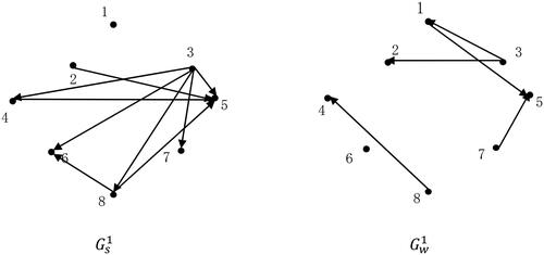
Step 5 The strong and weak outranking graphs are constructed based on the outranking relations shown in Step 4. The results are shown in Figure 1.

Figure 1. Strong outranking graph $G_s^1$ and weak outranking graph $G_w^1.$

Source: The Authors.

Step 6 The alternatives are then ranked in forward order and in reverse order.

1. Rank the alternatives in forward order.

As shown in Figure 1, the non-inferior alternative set in the strong graph $T_s^1=\left\{1,2,3\right\}$ and the non-inferior alternative set in weak graph $T_w^1=\left\{3,6,7,8\right\}$ are determined, with the intersection being $T^1=T_s^1\cap T_w^1=\left\{3\right\}$。

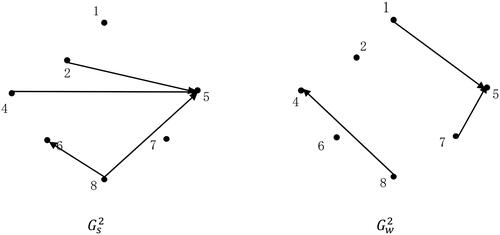
Alternatives $A_3$ and the related directed arcs are erased and the remaining two graphs respectively denoted $G_s^2$ and $G_w^2,$ as shown in Figure 2.

Figure 2. The strong outranking graph $G_s^2$ and the weak outranking graph $G_w^2.$

Source: The Authors.

The non-inferior alternative set $T_s^2=\left\{1,2,4,7,8\right\}$ and $T_w^2=\left\{1,2,6,7,8\right\}$ are then determined, with the intersection set being $T^2=T_s^2\cap T_w^2=\left\{1,2,7,8\right\}.$

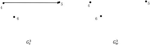
The alternatives in set $T^2$ and the directed arcs that start at these alternatives are then erased and the remaining two graphs in the outranking graph respectively denoted $G_s^3$ and $G_w^3,$ as shown in Figure 3.

Figure 3. The strong outranking graph $G_s^3$ and the weak outranking graph $G_w^3.$

Source: The Authors.

The non-inferior alternative set $T_s^3=\left\{4,6\right\}$ and $T_w^3=\left\{4,5,6\right\}$ are then determined, with the intersection set being $T^3=T_s^3\cap T_w^3=\left\{4,6\right\}.$

The alternatives in set $T^3$ and the directed arcs that start at these alternatives are then erased and the remaining two graphs in the outranking graph respectively denoted $G_s^4$ and $G_w^4,$ as shown in Figure 4.

Figure 4. The strong outranking graph $G_s^4$ and the weak outranking graph $G_w^4.$

Source: The Authors.

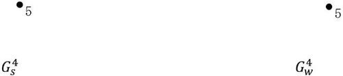
Finally, $T^4=\left\{5\right\}$ is determined.

Therefore, the forward order ${\phi }_1\left(A_i\right)$ of all alternatives is shown in Table 8.

Table 8. Forward order of all alternatives.

$A_i$	$A_1$	$A_2$	$A_3$	$A_4$	$A_5$	$A_6$	$A_7$	$A_8$
${\phi }_1\left(A_i\right)$	2	2	1	3	4	3	2	2

Source: The Authors.

1. Rank in reverse order

Using the same method and the Equations (22) – (23), we get the reverse orders ${\phi }_3\left(A_i\right)$ and the average order $\overline{\phi }(A_i),$ the results are shown in Table 9.

Table 9. Reverse order and average order of all alternatives.

$A_i$	$A_1$	$A_2$	$A_3$	$A_4$	$A_5$	$A_6$	$A_7$	$A_8$
${\phi }_3\left(A_i\right)$	3	3	1	3	4	4	3	2
$\overline{\phi }(A_i)$	2.5	2.5	1	3	4	3.5	2.5	2

Source: The Authors.

The final ranking order for all alternatives is determined as: $$A_3\succ A_8\succ A_1,A_2,A_7\succ A_4\succ A_6\succ A_5$$

Therefore, $A_3$ is superior to the other alternatives.

6. Conclusion

As a valid MCDM method, ELECTRE II is able to evaluate a set of alternatives using several criteria. In this paper, a PLTS-ELECTRE II method was proposed to solve MCDM problems, which was then applied to a typical MCDM venture capital project evaluation problem. A comprehensive venture capital project evaluation index system was constructed that included multiple qualitative and quantitative indicators, such as industry background, marketing, product technology, team management and financial data. In practical applications, qualitative attributes are generally PLTSs to allow for a reasonable evaluation. The sequence of alternatives was then determined using the PLTS-ELECTRE II method. In future studies, the developed PLTS-ELECTRE II method could be used to solve MCDM problems in other fields. Another future research direction could be determining new operations for linguistic term sets so that we could provide more precise assessment information for decision-making problems.

Disclosure statement

No potential conflict of interest was reported by the authors.

Additional information

Funding

This research was supported by the National Natural Science Foundation of China (no. 72001178), the Humanities and Social Sciences Foundation of the Ministry of Education of China (no. 17YJC630119). It was also supported by Applied Basic Research Program of Sichuan Province (no. 2020YJ0042) and the project of Research Center for System Sciences and Enterprise Development (no. Xq20B08).

References

- Akram, M., Adeel, A., Al-Kenani, A. N., & Alcantud, J. C. R. (2020). Hesitant fuzzy N -soft ELECTRE-II model: A new framework for decision-making. Neural Computing and Applications, 32, 1–16. https://doi.org/10.1007/s00521-020-05498-y.
- Alexopoulos, S., Siskos, Y., Tsotsolas, N., & Hristodoulakis, N. (2012). Evaluating strategic actions for a Greek publishing company. Operational Research, 12(2), 253–269. https://doi.org/10.1007/s12351-010-0092-0
- Batterson, L. A. (1986). Raising venture capital and the entrepreneur. McGraw Hill Professional.
- Benayoun, R., Roy, B., & Sussman, B. (1966). ELECTRE: Une méthode pour guider le choix en présence de points de vue multiples. Note de travail no. 49, Direction Scientifique de la SEMA.
- Celotto, A., Loia, V., & Senatore, S. (2015). Fuzzy linguistic approach to quality assessment model for electricity network infrastructure. Information Sciences, 304, 1–15. https://doi.org/10.1016/j.ins.2015.01.001
- Chen, N., & Xu, Z. (2015). Hesitant fuzzy ELECTRE II approach: A new way to handle multi-criteria decision making problems. Information Sciences, 292, 175–197. https://doi.org/10.1016/j.ins.2014.08.054
- Chen, T. (2020). New Chebyshev distance measures for Pythagorean fuzzy sets with applications to multiple criteria decision analysis using an extended ELECTRE approach. Expert Systems with Applications, 147, 113164. https://doi.org/10.1016/j.eswa.2019.113164
- Cheng, X., Gu, J., & Xu, Z. (2017). Venture capital group decision-making with interaction under probabilistic linguistic environment. Knowledge Based Systems, 140, 82–91.
- Coronado, M., Dosal, E., Coz, A., Viguri, J. R., & Andres, A. (2011). Estimation of construction and demolition waste generation and multi-criteria analysis of management alternatives: A case study in Spain. Waste & Biomass Valorization, 2(2), 209–225.
- Eckhardt, J. T., Shane, S., & Delmar, F. (2006). Multistage selection and the financing of new ventures. Management Science, 52(2), 220–232. https://doi.org/10.1287/mnsc.1050.0478
- Elshorbagy, A. (2006). Multi-criterion decision analysis approach to assess the utility of watershed modeling for management decisions. Water Resources Research, 420(9), 2286–2292.
- Ferreira, L., Borenstein, D., & Santi, E. (2016). Hybrid fuzzy MADM ranking procedure for better alternative discrimination. Engineering Applications of Artificial Intelligence, 50, 71–82. https://doi.org/10.1016/j.engappai.2015.12.012
- Gershon, M., Duckstein, L., & Mcaniff, R. (1982). Multi-objective river basin planning with qualitative criteria. Water Resources Research, 18(2), 193–202. https://doi.org/10.1029/WR018i002p00193
- Ghorabaee, M. K., Amiri, M., Zavadskas, E. K., & Antucheviciene, J. (2017). Supplier evaluation and selection in fuzzy environments: A review of MADM approaches. Ekonomska Istraivanja, 30(1), 1073–1118.
- Govindan, K., & Jepsen, M. B. (2016). ELECTRE: A comprehensive literature review on methodologies and applications. European Journal of Operational Research, 250(1), 1–29. https://doi.org/10.1016/j.ejor.2015.07.019
- Herrera, F., & Herrera-Viedma, E. (2000). Linguistic decision analysis: Steps for solving decision problems under linguistic information. Fuzzy Sets & Systems, 115(1), 67–82.
- Liang, W., Dai, B., Zhao, G., & Wu, H. (2019). Performance evaluation of green mine using a combined multi-criteria decision making method with picture fuzzy information. IEEE Access, PP(99), 1–1.
- Liao, H. C., Yang, L. Y., & Xu, Z. S. (2018). Two new approaches based on ELECTRE II to solve the multiple criteria decision making problems with hesitant fuzzy linguistic term sets. Applied Soft Computing, 63, 223–234. https://doi.org/10.1016/j.asoc.2017.11.049
- Liao, H., Jiang, L., Lev, B., & Fujita, H. (2019). Novel operations of PLTSs based on the disparity degrees of linguistic terms and their use in designing the probabilistic linguistic ELECTRE III method. Applied Soft Computing, 80, 450–464. https://doi.org/10.1016/j.asoc.2019.04.018
- Lin, M., Chen, Z., Xu, Z., Gou, X., & Herrera, F. (2021). Score function based on concentration degree for probabilistic linguistic term sets: An application to TOPSIS and VIKOR. Information Sciences, 551, 270–290. https://doi.org/10.1016/j.ins.2020.10.061
- Liu, Z., Zhao, X., Li, L., Wang, X., Wang, D., & Liu, P. (2020). Selecting a public service outsourcer based on the improved ELECTRE II method with unknown weight information under a double hierarchy hesitant linguistic environment. Sustainability, 12(6), 2315. https://doi.org/10.3390/su12062315
- Macmillan, I. C., Siegel, R., & Narasimha, P. N. S. (1985). Criteria used by venture capitalists to evaluate new venture proposals. Journal of Business Venturing, 1(1), 119–128. https://doi.org/10.1016/0883-9026(85)90011-4
- Mao, X. B., Wu, M., Dong, J. Y., Wan, S. P., & Jin, Z. (2019). A new method for probabilistic linguistic multi-attribute group decision making: Application to the selection of financial technologies. Applied Soft Computing, 77, 155–175. https://doi.org/10.1016/j.asoc.2019.01.009
- Mardani, A., Jusoh, A., Nor, K., Khalifah, Z., Zakwan, N., & Valipour, A. (2015). Multiple criteria decision-making techniques and their applications: A review of the literature from 2000 to 2014. Economic Research-Ekonomska Istraživanja, 28(1), 516–571. https://doi.org/10.1080/1331677X.2015.1075139
- Mason, C., & Stark, M. (2004). What do investors look for in a business plan? A comparison of investment criteria of bankers, venture capitalists and business angels. International Small Business Journal: Researching Entrepreneurship, 22(3), 227–248. https://doi.org/10.1177/0266242604042377
- Niu, D., Zhen, H., Yu, M., Wang, K., Sun, L., & Xu, X. (2020). Prioritization of renewable energy alternatives for China by using a hybrid FMCDM methodology with uncertain information. Sustainability, 12(11), 4649. https://doi.org/10.3390/su12114649
- Pang, Q., Wang, H., & Xu, Z. S. (2016). Probabilistic linguistic term sets in multi-attribute group decision making. Information Sciences, 369, 128–143. https://doi.org/10.1016/j.ins.2016.06.021
- Rodríguez, R. M., Martı́nez, L., & Herrera, F. (2012). Hesitant fuzzy linguistic term sets for decision making. IEEE Transactions on fuzzy systems, 20(1), 109–119. https://doi.org/10.1109/TFUZZ.2011.2170076
- Roy, B. (1968). Classement et choix en présence de points de vue multiples. Revue Française D'informatique et de Recherche Opérationnelle, 2(8), 57–75. https://doi.org/10.1051/ro/196802V100571
- Roy, B., & Bertier, P. (1973). La methode ELECTRE II: une methode au media-planning. Operational Research, 1973(72), 291–302.
- Shumaiza, Akram M., & Al-Kenani, A. N. (2019). Multiple-attribute decision making ELECTRE II method under bipolar fuzzy model. Algorithms, 12(11), 226.
- Smitham, P. (1990). Down the venture capital route. Accountancy, 106(10), 74–77.
- Tyzoon, T. T., & Bruno, A. V. (2011). A model of venture capitalist investment activity. Management Science, 30(9), 1051–1066.
- Wells, W. A. (1974). Venture capital decision-making. University Microfilms.
- Xu, J., & Shen, F. (2014). A new outranking choice method for group decision making under Atanassov’s interval-valued intuitionistic fuzzy environment. Knowledge-Based Systems, 70, 177–188. https://doi.org/10.1016/j.knosys.2014.06.023
- Yue, C. Y. (2003). Decision theory and method. Science Press.
- Zadeh, L. A. (1975). The concept of a linguistic variable and its application to approximate reasoning - II. Information Sciences, 8(4), 301–357. https://doi.org/10.1016/0020-0255(75)90046-8
- Zider, B. (1998). How venture capital works. Harvard Business Review, 76(6), 131–139.