How do firms form inflation expectations? Empirical evidence from the United States

Abstract

Inflation expectations of firms affect their micro-decision-making behaviors and therefore impact the macro-economy. Thus, a deep understanding of how firms form inflation expectations benefits the achievement of central bank’s policy objectives on macro-economic sustainability and development. In this paper, we focus on the inflation expectations of firms from surveys. Specifically, the Naïve Expectation, Adaptive Expectation, Rational Expectation, VAR, and Heterogeneous Static Expectation formation models are adopted to test the models being used by firms to form inflation expectations. Empirically, this paper reveals the heterogeneity between the formation mechanisms of households and firms. Then, empirical results reject the rational expectation hypothesis of firms’ inflation expectations, which means that they are not perfectly rational. Finally, we find that the inflation perception is a non-negligible factor in forming firms’ inflation expectations. Therefore, central banks’ monetary policies that aiming to formulate firms’ inflation perceptions can be a useful tool in regulating their inflation expectations, which are expected to benefit the stability of the macro-economy.

Keywords:

• Inflation expectations
• firm
• heterogeneity
• inflation perception
• monetary policy

JEL Codes:

• E31; E17; E3

1. Introduction

The inflation expectation is the core of current macro-economic research as it affects the economy through its influences on the actual inflation (Rudd & Whelan, 2007). Thus, the inflation expectation attracts numerous investigations in the macroeconomic field, e.g., the macro-finance term structure (Gomez-Cram & Yaron, 2017) and the spillover in global financial uncertainty (Ghosh et al., 2020). Economic agents are inherently different in affecting the macro economy. Thereby, inflation expectations can also be divided into three types, i.e., households, firms, and professional forecasters (Coibion et al., 2018). Tremendous studies focus on inflation expectations of households and professional forecasters; however, the research on firms’ inflation expectations, which is the decisive factor regarding the most important paradigm in analyzing the macro economy, i.e., the New Keynesian Phillips Curve (NKPC), appears to be limited. Firms’ inflation expectations are expected to be more important than that of households and professional forecasters because of their unique role in pricing decisions and labour markets. For example, Kaihatsu and Shiraki (2016) argue that both wages and short-term inflation expectations of firms tend to increase along with medium- to long-term inflation expectations. Besides, they illustrate that wages and operating profits tend to decrease when only short-term inflation expectations increase. Consequently, investigating the formation of firms’ inflation expectations and making comparisons with households are enlightening for central banks in structuring monetary policies.

Lyziak (2014) reports a significant difference between inflation expectations of firms and individual consumers and attributes such difference to information sets and expectation formation models. A further in-depth study of Lyziak (2016) suggests that compared with expectations of consumers or profession forecasters, firms’ expectations are more appropriate to explain and forecast the real economy. Unfortunately, there is limited research directly studying the formation mechanism of firms’ inflation expectations, which leaves a significant empirical gap for firms’ inflation expectations. In this paper, we focus on the inflation expectation of firms and, specifically, investigate the formation mechanism of their expectations. Based on the seminal works of Mankiw et al. (2003) and Sims (2003), the imperfect information theory is adopted in this paper to analyze the formation mechanism of firms’ inflation expectations.

Regarding the formation mechanism, previous studies propose many different models regarding inflation expectations of individuals and professional forecasters, e.g., the Rational Expectation (RE), Static Expectation (SE), and Adaptive Expectation (AE) (Bernanke et al., 2004; Cagan, 1956; Muth, 1961). Nevertheless, empirical results conflict with theories that assume a single formation mechanism for all agents. Instead, there are evidence suggesting that the formation of inflation expectations regards more than one of the above theories (Brock & Hommes, 1997; Mankiw & Reis, 2002; Sims, 2003). Thus, the heterogeneity in adopting inflation expectation formation models attracts much attention since then. Brock and Hommes (1997) choose a set of available predictors and establish an Adaptive Rational Dynamic Equilibrium (ARDE) model to investigate the formation of inflation expectations. Branch (2004) further proposes the Rational Heterogeneous Expectations (RHE) theory based on the ARDE model. An in-depth study of Branch (2007) confirms the important assumption agreeing with the RHE that the probability of one predictor being selected is negatively correlated with the mean square deviation of inflation and the cost of the potential predictor. Subsequently, Maag (2010) proposes a heterogeneous static expectation (HSE) model and shows that the inflation perception is the primary factor in updating households’ inflation expectations using a Mixture Gauss Model. The study of Xu et al. (2016) proposes a Heterogeneous Adaptive Expectation (HAE) model which includes the real inflation, past inflation expectations, and inflation perceptions as factors affecting inflation expectations. Bräuning and van der Cruijsen (2019) investigate the learning dynamics of inflation expectations in six European countries and point out that the learning rules of inflation expectations vary over countries and times. However, all the above-mentioned studies focus on households’ inflation expectations. The importance of firms’ inflation expectations on the macro-economy has long been ignored by empirical studies. Hubert and Mirza (2019) point out that longer term expectations are crucial in shaping shorter horizon expectations. The study of Nakazono (2020) further argues that disagreements on inflation forecasts among households are larger for the shorter-term than those for the longer-term horizon.

Fortunately, the enrichment on survey data about firms’ inflation expectations attracts recent attention. For example, Lyziak (2013) and Kabundi et al. (2015) report significant empirical differences between inflation expectations of households and firms. Bryan et al. (2015) and Coibion and Gorodnichenko (2015) suggest that firms’ inflation expectations and their inflation perceptions are highly correlated. Based on the business trend survey in Slovakia, the study of (2015) examines whether firms completely adopt the Rational Expectation theory when forming expectations. Uno et al. (2018) hold the view that firms' inflation expectations are downwardly rigid. Bottone and Rosolia (2019) find that unanticipated changes in market rates are negatively correlated in a statistically significant way with the differences in inflation expectations between two groups of firms and that this effect has become stronger since 2009 in Italy. Besides, the results show that inflation expectations of firms in Italy can quickly response to the shocks from monetary policies. Based on the data of firms in Japan, Kitamura and Tanaka (2019) indicate that the formation of firms’ inflation expectation is complex. Furthermore, although firms' inflation expectations have been pushed up by the Bank of Japan's introduction of its "price stability target" and the expansion in the output gap amid the Bank's Quantitative and Qualitative Monetary Easing (QQE), the presence of rational inattention and information stickiness has slowed the pace of the rise in firms' inflation expectations. The empirical results of Nosratabadi (2020) confirm that firms' inflation expectations are not consistent with the full-information rational expectations models.

Even so, to the best of our knowledge, the formation mechanism of firms’ inflation expectations has not been revealed yet, which constitutes the most important issue in this study. Following the empirical investigation of Branch (2004) which regards households’ inflation expectations, we consider both inflation expectations of households and firms and make comprehensive comparisons between two groups. This paper makes the following contributions to the literature. First, we focus on the heterogeneity between the formation mechanisms of households and firms. The empirical results indeed suggest a significant heterogeneity. Second, we test whether the inflation expectation of firms is rational. The results suggest that firms’ inflation expectations are not perfectly rational. Finally, we reveal the effect of inflation perceptions on firms’ inflation expectations.

The rest of this paper is organised as follows. Section 2 introduces some models in explaining the formation of inflation expectations. Section 3 shows the data and methodologies in analyzing the heterogeneity in model selection. Section 4 presents the empirical results, and Section 5 concludes this paper.

2. Potential models in forming inflation expectations

2.1. Naïve expectation

The Naive Expectation (NE) is based on the cobweb theory, which assumes that economic participants expect the latest inflation expectation to be the actual inflation in the current time. If economic agents form the inflation expectation by the Naïve Expectation theory, the cost will be low as the actual inflation is published officially each month. According to the theory, the inflation expectation can be generalised by the following equation: (1) $${\pi }_{t+\Delta \mathrm{t}|t}^{e,N}={\pi }_t$$(1) where ${\pi }_t$ is the actual inflation in time t, and ${\pi }_{t+\Delta \mathrm{t}|t}^{e,N}$ is the inflation expectation for time $\left(t+\Delta \mathrm{t}\right)$ made by agents in time t.

2.2. Adaptive expectation

The Adaptive Expectation (AE) assumes that the information in the past plays a nonnegligible role in the formation of inflation expectations. According to the theory, inflation expectations of the future depend on two factors. The first factor refers to the inflation expectation made in the past period, and the second part refers to the error between the actual inflation and the first factor. The inflation expectation of the future is a linear weighted average of the two parts. In this sense, despite of the linear format, the Adaptive Expectation appears to be more sophisticated than the Naïve Expectation. The formation mechanism can be generalised by the following equation: (2) $${\pi }_{t+\Delta \mathrm{t}|t}^{e,A}={\pi }_{t|t-\Delta \mathrm{t}}^{e,A}+\gamma \left({\pi }_t-{\pi }_{t|t-\Delta \mathrm{t}}^{e,A}\right)=\mathrm{\gamma }{\pi }_t+\left(1-\gamma \right){\pi }_{t|t-\Delta \mathrm{t}}^{e,A}$$(2) where ${\pi }_t$ and ${\pi }_{t+\Delta \mathrm{t}|t}^{e,N}$ are the same as in Equation (1)(1) $${\pi }_{t+\Delta \mathrm{t}|t}^{e,N}={\pi }_t$$(1) , and ${\pi }_{t|t-\Delta \mathrm{t}}^{e,A}$ is the inflation expectation in month t made by individuals in time t-$\Delta \mathrm{t}.$ Thus, the ${\pi }_t-{\pi }_{t|t-\Delta \mathrm{t}}^{e,A}$ is the error term between the actual inflation and the corresponding expectation. $\gamma \in [0,1]$ denotes the parameter to revise expectation.

2.3. Var model

Based on the classical prediction technology, i.e., the Vector Autoregression model (VAR), Branch (2004) puts forward the VAR predictor in inflation expectations. The VAR predictor regards the inflation forecast as the inflation expectation. The VAR predictor has the similar framework with the VAR model. The VAR predictor reduces the influence of incomplete information and costs on inflation expectations, thus is widely used in previous studies. Both two methods assume a stationary condition for the selected series. Similarly, the VAR predictor forecasts the inflation expectation by the past inflation expectations and many other related variables. Specifically, in this paper, we select the monthly actual inflation, the monthly unemployment rate, the monthly growth rate of M1, the monthly London Interbank Offered Rate (LIBOR) and inflation expectations to construct the VAR model.

Comparing with the Naïve Expectation and Adaptive Expectation, the VAR predictor is impressive because of its inclusion of many other macro-economic variables. However, the information of central bank is moderately private, because the objectives are only partially credible for economic individuals, which makes it difficult to form a stable inflation expectation equilibrium in the actual economic operation. Thus, it is reasonable for agents to combine the historical track of monetary policy and the trend of economic variables to form inflation expectations. The VAR predictor can be generalised as follows: (3) $$y_t=\alpha +{\mathrm{\Omega }}_1{y}_{t-1}+{\mathrm{\Omega }}_2{y}_{t-2}+\dots +{\mathrm{\Omega }}_p{y}_{t-p}+u_t$$(3) where $y_t$ is a vector of the actual inflation and other related variables, $\alpha$ is a constant, ${\mathrm{\Omega }}_j\mathrm{}(\mathrm{j}=1\cdots \mathrm{p}$) represents the parameters, and $u_t$ is the error term which follows a normal distribution.

2.4. Rational expectation

The Rational Expectation theory assumes that all participants involved in economic activities make the best use of their information in forming expectations to avoid systematic mistakes. In this sense, the inflation expectation for time t+$\Delta \mathrm{t}$ made in time t is exactly supposed to be equal to the actual inflation at time t+$\Delta \mathrm{t}.$ The rational expectation can be expressed as follows: (4) $${\pi }_{t+\Delta \mathrm{t}|t}^{e,R}={\pi }_{t+\Delta \mathrm{t}}$$(4)

Theoretically, rational expectations are impossible with an unknown true distribution for the economy. However, expectations that result from a learning rule that shares the same structure as rational expectations or a proportion of agents that behave like economic forecasters are still possible (Evans & Honkapohja, 2012). Hence, for comparison, we include the Rational Expectation model into the predictor set.

2.5. Heterogeneous static expectation

The Heterogeneous Static Expectation model proposed by Maag (2010) emphasises the importance of inflation perceptions in forming inflation expectations. This theory argues that inflation expectations regarding the future equal to the current inflation perception: (5) $${\pi }_{t+\Delta \mathrm{t}|t}^{e,H}={\pi }_t^p$$(5) where ${\pi }_t^p$ is the inflation perception in time t. Agents can form heterogeneous inflation expectations because their personal inflation perceptions vary across agents. For a certain individual, it is practical to have his/her answer for the inflation perception through surveys. It should be noted that it is possible for households to give the same answer to perceived and expected inflations when an agent adopts another predictor that coincidentally generates an inflation expectation that equals to the perception.

3. Data and methodologies

3.1. Data

According to Branch (2004) which investigates a similar issue of households’ inflation expectations, certain questions within a survey regarding inflation or costs are adequate to measure agents’ inflation expectations. Hence, in this paper, due to data availability and previous investigations (Steindel & Deitz, 2005), the following data source regarding service prices of firms is adopted to measure firms’ inflation expectations. We collect our data from the Fifth District Survey of Service Sector Activity (FDSSSA), which is monthly implemented by the Federal Reserve Bank of Richmond in the United States. In this survey, about 200 firms receive questionnaires on several questions each month since November 1993, e.g., income, employment, wages, and prices etc. These companies are required to answer the following question which regards inflation expectations: during the next 6 months, do you think that services prices received will go up, down, or stay where they are now? While this survey focusses on the service sector, the data from Bureau of Economic Analysis suggest that growth trends of goods and services are closely related (Schnorbus & Watson, 2010). Meanwhile, the research of (Pinto et al., 2016) finds that the diffusion indices reported by this survey well capture the aggregate changes in a series of interest. For example, the employment diffusion index reported by this survey accounts for the bulk of changes in aggregate employment growth. Furthermore, this survey is the only source for such data on a timely enough basis to examine the formation of firms’ inflation expectations.

Specifically, we use the diffusion index as the basis to measure firms’ inflation expectations. The diffusion index is calculated by subtracting the percentage of agents choosing “go down” from the percentage of agents choosing “go up”. Seasonal adjustments are made every July to better reflect current economic trends. In measuring firms’ inflation expectations, we resort to the net balance statistic (Xu et al., 2021) which implies that the inflation expectation is positively correlated with the diffusion index with a constant coefficient. The net balance statistic is commonly used in the economic sentiment survey analysis and in measuring households’ inflation expectations. The seasonal adjustments are chosen for the following reason that “the non-seasonally adjusted expected demand index for the overall service sector was generally reported at a lower level than it should have been, understating the actual value of the inde^x”.1 Households’ inflation expectations are collected from the surveys of consumers implemented by the Survey Research Center at the University of Michigan. The surveys ask consumers questions regarding their current and future financial standings and their thoughts on the economy at the present time and in the near future. Similarly, we adopt the seasonally adjusted data. The report includes analysis of the survey results and indices for consumer sentiment and consumer expectations. The surveys have long stressed the important influence of consumer spending and saving decisions in determining the course of the national economy.

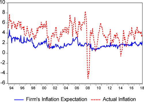
Figure 1 shows the movements of firms’ inflation expectations and corresponding actual inflation rates from November 1993 to June 2018. Several interesting discoveries can be observed from Figure 1. Specifically, the inflation expectation shows a decreasing trend during the sample period, whereas no significant trend for the actual inflation exists. The actual inflation is more violate compared with the inflation expectation. Meanwhile, the inflation expectation is positive which shows that the whole society is optimistic about the economic development. When the economy runs smooth, the tendency of firms’ inflation expectations consists with the actual inflation. For example, the two series show an increasing trend during the second half of 1998 to the first half of 2000. When the economy is in turmoil, the relationships appear to be unclear. For example, when the unanticipated financial crisis occurred in 2008, the actual inflation decreased sharply. However, the firms’ inflation expectation showed no significant change. With the development of the financial crisis, the inflation expectation began to respond to the crisis and showed a downward trend. Consequently, changes in inflation expectations may have resulted in the severe decrease of the actual inflation in 2009.

Figure 1. The actual inflation and firms’ inflation expectations in the United States. Source: Authors’ calculation.

3.2. Estimate predictor selection proportions

The costs of the above-mentioned predictors are non-negative, which are positively related to the difficulties of information obtaining and processing (Branch, 2004). Due to the difference in information collection and procession of individuals, the cost of a certain predictor varies, resulting in the difference in selecting predictors. We further define the net profit of using a predictor as the return minus the cost and assume that the proportion of a certain predictor being used is positively related with the net profit. Following Branch (2004), the general model for predictor selection can be generalised as follows.

Let $U_{j,t}$ denote the relative net profit of predictor j at time t. We allow agents to switch among predictors in different periods. The proportion of agents using predictor j in time t can be expressed as: (6) $${\eta }_{j,t}=\frac{\hspace{0.17em}\text{exp}\hspace{0.17em}\left(\beta U_{j,t}\right)}{{\sum }_{l=1}^K\hspace{0.17em}\text{exp}\hspace{0.17em}\left(\beta U_{l,t}\right)}\mathrm{}\mathit{for}\mathrm{}j=1,2,\dots ,K$$(6) where $\beta$ denotes the parameter for “intensity of choice’. A larger value of $\beta$ denotes that the agent tends to switch to this predictor because of the change in the relative net profit. A large enough β, i.e., β = +∞, means that ${\eta }_{j,t}$ becomes very large for the predictor with the highest success, that is, rational expectations. In contrast, a small β indicates that the survey data on inflation expectations is not perfectly rational. This finding is in line with Puah et al. (2017) that the business expectations in the construction sector is inconsistent with rational expectations.

According to the definition of $U_{j,t},$ it can be calculated as follows: (7) $$U_{j,t}=S_{j,t}-C_j$$(7) where $S_{j,t}$ represents the return of predictor j in time t, $C_j$ is the cost of predictor j which is assumed to be a constant. As mentioned above, a certain predictor may represent different costs to individuals. However, to simplify the estimation process, we assume $C_j$ to be a constant which equals to the average cost of individuals. The return in Equation (7)(7) $$U_{j,t}=S_{j,t}-C_j$$(7) , i.e., $S_{j,t},$ is calculated as follows: (8) $$S_{j,t}=-{\mathit{MSE}}_{j,t}$$(8) where MSE is the operator for mean square error and is obtained by (9) $${\mathit{MSE}}_{j,t}=\left(1-\delta \right){\mathit{MSE}}_{j,t-\Delta \mathrm{t}}+\delta {\left({\pi }_{j,t|t-\Delta \mathrm{t}}^e-{\pi }_t\right)}^2$$(9) where ${\pi }_{j,t|t-\Delta \mathrm{t}}^e$ is the inflation expectation at month t using predictor j that is made by agents in time $\left(t-\Delta \mathrm{t}\right),$ and ${\pi }_t$ is the actual inflation in time t. As shown in the above model specification, ${\mathit{MSE}}_{j,t}$ is a weighted average of the past value and the squared error term. Thus, the net profit can be expressed as follows: (10) $$U_{j,t}=-\left({\mathit{MSE}}_{j,t}+C_j\right)$$(10)

Accordingly, the probability of an agent adopting predictor j, which is also the proportion of agents selecting the predictor j, is given by the following equation. (11) $${\eta }_{j,t}=\frac{\hspace{0.17em}\text{exp}\hspace{0.17em}\left\{\beta \left[-\left({\mathit{MSE}}_{j,t}+C_j\right)\right]\right\}}{{\sum }_{l=1}^K\hspace{0.17em}\text{exp}\hspace{0.17em}\left\{\beta \left[-\left({\mathit{MSE}}_{l,t}+C_l\right)\right]\right\}}$$(11)

The proportion for each expectation predictor can thus be estimated through determining the parameters $\beta ,$ $\delta ,$ and $C_j.$ We assume that individuals choose from the predictors set to form their personal inflation expectations. Differences originated from individuals result in deviations between survey results and estimates of predictors. Under the assumption that the forecast errors, i.e., deviations between expectations and estimates of predictors, are normally distributed, we establish the likelihood function of individual survey expectations as follows.

The actual observed survey expectations are represented by (12) $${\pi }_{i,t+\Delta \mathrm{t}|t}^e=H_j\left({\pi }_t\right)+v_{it}$$(12) where $v_{it}\sim N\left(0,{\sigma }_v^2\right),$ $H_j$ is the selected predictor of an individual. Since $v_{it}$ follows a normal distribution, the density of ${\pi }_{i,t+\Delta \mathrm{t}|t}^e$ can be calculated as follows: (13) $$\mathrm{P}\left({\pi }_{i,t+\Delta \mathrm{t}|t}^e|{\mathit{MSE}}^t\right)={\sum }_{l=1}^K{n}_{l,t}P\left({\pi }_{i,t+\Delta \mathrm{t}|t}^e|j=l\right)$$(13) (14) $$P\left({\pi }_{i,t+\Delta \mathrm{t}|t}^e|j\right)=\frac{1}{\sqrt{2\pi }{\sigma }_v}\text{exp}\hspace{0.17em}\left\{-\frac{1}{2}{\left[\frac{{\pi }_{i,t+\Delta \mathrm{t}|t}^e-H_j\left({\pi }_t\right)}{{\sigma }_v}\right]}^2\right\}$$(14)

Thus, the probability of the sample is provided by: (15) $$\mathrm{P}\left({\pi }_{i,t+\Delta \mathrm{t}|t}^e|{\mathit{MSE}}^t,{\mathcal{H}}_t({\pi }_t)\right)=\prod _t\prod _i\left[{\sum }_{l=1}^K{n}_{l,t}P\left({\pi }_{i,t+\Delta \mathrm{t}|t}^e|j=l\right)\right]$$(15) where $i=1,\dots ,N$ and $t=1,\dots ,T.$ The maximised log-likelihood estimate of the density function is (16) $$\mathcal{L}=\sum _t\sum _{i}ln{\sum }_{l=1}^K{\eta }_{l,t}\times P\left({\pi }_{i,t+\Delta \mathrm{t}|t}^e|l\right)$$(16) where ${\eta }_{l,t}=\frac{\hspace{0.17em}\text{exp}\hspace{0.17em}\left\{\beta \left[-\left({\mathit{MSE}}_{l,t}+C_l\right)\right]\right\}}{{\sum }_{k=1}^K\hspace{0.17em}\text{exp}\hspace{0.17em}\left\{\beta \left[-\left({\mathit{MSE}}_{k,t}+C_k\right)\right]\right\}}.$

The above equation shows that the likelihood value of the survey expectation depends on the mean square errors, cost, and a normally distributed random disturbance. The objective is to estimate parameters of $\beta ,$ ${\sigma }_v,$ and $C_j.$ To make comparisons with Branch (2004), we set the number of models included in a predictor set to be three, and normalise the cost of one of them to zero, which has no essential effect on the results.

Empirically, in measuring the prediction accuracy, we refer to the difference between monthly actual inflation and expectations generated by predictors. We assume that agents input monthly actual inflation data to generate inflation expectations because this is the way the media reports inflation (Branch, 2004). However, the theory claims that agents are concerned with annual forecasts and should therefore discount very noisy monthly data. We consider these two hypothetical agents responding to both the recently observed prediction errors and the damping of past prediction errors. In the empirical study, we choose the following prediction errors that produces the most accurate results. (17) $${\mathit{MSE}}_{j,t}=\left[{\mathit{MSE}}_{j,t-\Delta \mathrm{t}}^{\delta =1},{\mathit{MSE}}_{j,t-3\Delta \mathrm{t}}^{\delta =0.9}\right]$$(17) where ${\mathit{MSE}}_{j,t-\Delta \mathrm{t}}^{\delta =1}={\left({\pi }_{m,t-\Delta \mathrm{t}}-{\pi }_{j,t-2\Delta \mathrm{t}}\right)}^2$ and ${\mathit{MSE}}_{j,t-3\Delta \mathrm{t}}^{\delta =0.9}=0.1\times {\mathit{MSE}}_{j,t-3\Delta \mathrm{t}}^{\delta =0.9}+0.9\times {\left({\pi }_{m,t-2\Delta \mathrm{t}}-{\pi }_{j,t-3\Delta \mathrm{t}}\right)}^2.$ ${\mathit{MSE}}_{j,t-\Delta \mathrm{t}}^{\delta =1}$ is the prediction error of model j based on the recent inflation. ${\mathit{MSE}}_{j,t-3\Delta \mathrm{t}}^{\delta =0.9}$ is the geometrically weighted average of all past prediction errors². Performance measures with inertia such as these are considered by Branch and McGough (2004) and Branch and Evans (2006). Therefore, we allow agents to adjust their choices according to new and past information.

4. Empirical results

4.1. Inflation expectation formations based on naïve expectation, adaptive expectation, and VAR models

Inflation expectations of firms and households are heterogeneous (Kaihatsu & Shiraki, 2016; Lyziak, 2013). However, there are few studies focussing on the issue of whether the mechanisms of inflation expectations are heterogeneous, i.e., the formation of inflation expectations. To solve this problem, we estimate the proportions of different agents in using a certain inflation expectation formation model through measuring the proportions of models being used by a certain group. We follow Branch (2004) and set the potential predictors to include the Naïve Expectation, the Adaptive Expectation, and the VAR model. For both firms and households, we assume that they choose from the predictor set when forming personal inflation expectations. Thus, the predictor set ${\mathcal{H}}_0\left({\pi }_{t|t-\Delta \mathrm{t}}^e\right)=\left\{{\pi }_{t|t-\Delta \mathrm{t}}^{e,N},\mathrm{}{\pi }_{t|t-\Delta \mathrm{t}}^{e,A},\mathrm{}{\pi }_{t|t-\Delta \mathrm{t}}^{e,V}\right\},$ where ${\pi }_{t|t-\Delta \mathrm{t}}^{e,N}$ means the naive predictor, ${\pi }_{t|t-\Delta \mathrm{t}}^{e,A}$ represents the adaptive expectation predictor, and ${\pi }_{t|t-\Delta \mathrm{t}}^{e,V}$ refers to the VAR predictor.

Limited by data availability, we choose the time period from January 1978 to June 2018 to estimate the formation specifications of households. For firms, we set the sample period to cover November 1993 to June 2018. For comparison, we also estimate the proportions of households in using a certain predictor during November 1993 to June 2018. On the one hand, changes in the sample periods for households enable us to test the robustness of the method. On the other hand, results for firms and households during the same period reveal the heterogeneity between two groups. Table 1 reports the stationarity tests for inflation expectations of households and firms and the actual inflation during November 1993 to June 2018. Both methods of the augmented Dickey–Fuller (ADF) unit root test (Dickey & Fuller, 1981) and the Phillips and Perron’s test (Phillips & Perron, 1988) suggest that the target variables are stationary.

Table 1. Stationarity tests for inflation expectations and actual inflation.

Unit root test method	Inflation Expectation		Actual Inflation
	Firm	Household
ADF	−3.5977 (0.0064)	−3.7190 (0.0225)	−3.3955 (0.0119)
PP	−4.4274 (0.0003)	−5.3151 (0.0001)	−4.8671 (0.0001)

Note: This table summarises the stationarity test results of inflation expectations of firms and households and the actual inflation. ADF denotes the augmented Dickey–Fuller (ADF) unit root test and PP denotes the Phillips and Perron’s test. The sample period is November 1993 to June 2018.

Source: Authors’ calculation.

For simplicity, we normalise the cost of the naïve predictor to be zero, which has no essential effect on the estimation results. The first two rows in Table 1 summarise the estimation results of coefficients of ${\mathit{MSE}}_{j,t-\Delta \mathrm{t}}^{\delta =1}$ and ${\mathit{MSE}}_{j,t-\Delta \mathrm{t}}^{\delta =0.9},$ which represent the recent prediction error and past errors, respectively. The last three rows of Table 1 report the costs of corresponding predictor.

According to Table 2, the coefficient for the recent prediction error is much larger than that for the past error for households in different periods. Specifically, the coefficient for the recent prediction error is 0.0333, whereas the value is 0.1348 for the past error during January 1978 to June 2018. During November 1993 to June 2018, the coefficients for the recent and past prediction errors are 0.0127 and 0.1036, respectively. Both two panels show that households’ response to dampened past errors is stronger than that of recent prediction errors. From Panel C, the coefficient for the recent forecast error (0.1857) is larger than that for the past forecast error (0.1019). Thereby, contrary to households, the impact of recent forecast errors on firms’ inflation expectations is greater than that of dampened past errors. Besides, the results of a finite coefficient for the forecast errors indicate that inflation expectations of firms are not perfectly rational. Additionally, the coefficients shown in Panel C are larger than that of Panel B, which shows that firms are more rational in forming inflation expectations than households.

Table 2. Maximum likelihood estimates for households and firms with the naïve expectation, adaptive expectation, and VAR model.

	Panel A	Panel B	Panel C
	Households (1978.1-2018.06)	Households (1993.11-2018.06)	Firms (1993.11-2018.06)
${\mathit{MSE}}_{j,t-\Delta \mathrm{t}}^{\delta =1}$	0.0333 (0.0001)	0.0127 (0.0247)	0.1857 (0.0000)
${\mathit{MSE}}_{j,t-3\Delta \mathrm{t}}^{\delta =0.9}$	0.1348 (0.0000)	0.1035 (0.0000)	0.1019 (0.0000)
$C_N$	0.0000	0.0000	0.0000
$C_A$	26.7892 (0.0030)	12.9568 (0.0015)	−143.9588 (0.0006)
$C_V$	−19.3604 (6.2542)	−16.5925 (5.3600)	−150.9925 (0.1017)

Note: $C_N,$ $C_A,$ and $C_V$ represent the costs of naïve, adaptive, and VAR predictors, respectively. Standard errors in parentheses.

Source: Authors’ calculation.

Turning to the cost of each inflation expectation predictor, we find that the adaptive predictor is the most expensive for households, followed by the naïve predictor. Surprisingly, the VAR predictor, rather than the naïve expectation, has the lowest cost. This appears to disagree with our previous assumption that the cost is proportional to the ‘complexity’ of the predictor. However, the cost can be treated as a predisposition to use a certain predictor (Branch, 2004). Thus, the results just indicate that households prefer to form inflation expectations by the VAR predictor. For firms, the cost of the naïve predictor is the highest, followed by the adaptive expectation and the VAR predictor. Similarly, this result indicates that firms prefer the VAR model and the adaptive expectation in forming inflation expectations. By comparing the empirical results in Panels B and C which cover the same period, one can find that both households and firms believe that the VAR predictor has the lowest cost. In terms of the naïve predictor and the adaptive expectation, households prefer the naïve predictor, whereas firms believe that the adaptive expectation has a lower cost.

Figures 2-4 show the proportions of each predictor being adopted by households and firms which correspond to the settings in Panels A, B, and C. According to Figure 2, the VAR model is the best explanation of the way in which these expectations are formed. This indicates that most households use the VAR predictor to form personal inflation expectations, whereas only a few agents adopt the Adaptive Expectation. Similar results can also be found in Figure 3, which shows that the best model maintains in different periods. In other words, households tend to maintain the way in forming inflation expectations in different periods. Figure 2 shows that, generally, 97% of households use the VAR predictor to generate inflation expectations. Nearly 3% of households adopt the naïve predictors. Less than 0.1% of households adopt the Adaptive Expectation. From Figure 3, the proportion of households in using the VAR predictor declines slightly; but still dominates the other two models with approximately 90% of households adopting it. Similarly, the proportions of households using the naïve predictor and the adaptive expectation rank the second and the last. Slight difference between two periods shown in Figures 2 and 3 can be attributed to the switch among agents. For a certain agent who prefers the VAR predictor, she/he may find that it is worthwhile to change the model in forming expectations when the prediction error reaches the threshold. For example, when the naïve predictor is expected to have a better prediction accuracy, the agent using the VAR predictor may switch.

Figure 2. The proportions of the Naïve Expectation, Adaptive Expectation, and VAR model for households (January 1978 to June 2018). Source: Authors’ calculation.

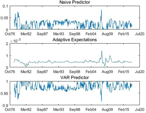
Figure 3. The proportions of the Naïve Expectation, Adaptive Expectation, and VAR model for households (November 1993 to June 2018). Source: Authors’ calculation.

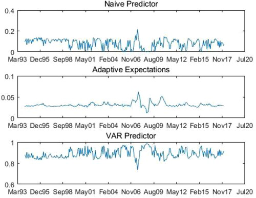
Figure 4. The proportions of the Naïve Expectation, Adaptive Expectation, and VAR model for firms (November 1993 to June 2018). Source: Authors’ calculation.

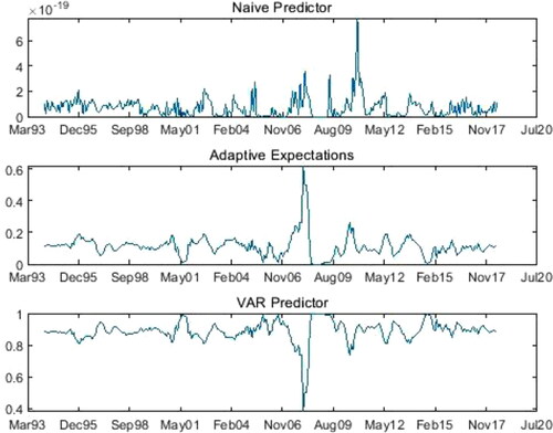
According to Figure 4, for firms, the VAR predictor dominates the other models, followed by the Adaptive Expectation and the Naïve Expectation. This finding is significantly different from the case of households for which the Adaptive Expectation cannot explain well the formation of inflation expectations. Thereby, it seems that only a few agents adopt the Adaptive Expectation. The similarity on the preference for the VAR predictor does not necessarily mean that the inflation expectation formation models are the same for households and firms. Instead, this can be attributed to the following reasons. First, the expected future period of them is different. According to the surveys, the firm expresses the expectation for the next six months, whereas the households report the expectations for the next year. Second, although the proportions of the VAR model for two groups are similar, there are differences in the perception of recent prediction errors and dampened past errors. Finally, similar results may be because of the cost of the current predictor has not yet reached the threshold of changing the predictor. Panels A and B further show that the selection of predictors changes over time. Once the prediction error reaches the threshold, agents may switch to another predictor.

The proportions of using the Adaptive Expectation are different for households and firms, which shows that firms are more focussed on correcting past errors than households. The differences in Figures 3 and 4 indicate a significant heterogeneity between households and firms in inflation expectation formation models. The empirical results may further indicate that, in macro-economic analysis and monetary policy formulation, replacing firms’ inflation expectations with households’ inflation expectations is likely to cause large deviations.

As shown in Figures 2 and 3, extreme values occurred between 2007 and 2008. During the financial crisis period, the proportion of firms in using the VAR predictor declines dramatically, whereas the proportions of using the naïve predictor and the Adaptive Expectation increase. This phenomenon can be attributed to the overreaction of agents to the subprime mortgage crisis and the financial crisis. When the market changes sharply, agents tend to focus more on current information and ignore past information. Besides, it may also be concluded that firms are more sensitive to shocks than households as the magnitude of proportion changes is greater for firms.

Overall, we find that the proportions for a certain inflation expectation formation model of firms and households changes over time. Generally, both firms and households prefer the VAR predictor to the Naïve Expectation and the Adaptive Expectation in forming inflation expectations

4.2. Firms’ inflation expectation formations based on alternative models

n the above section, we adopt the potential predictors set following Branch (2004) and conclude that firms prefer the VAR predictor than the other two models. However, the selection of predictors set may be incomplete. The Rational Expectation and the Heterogeneous Static Expectation provide another two important and widely used formation mechanisms. The Rational Expectation is the foundation of numerous economic theories, whereas the Heterogeneous Static Expectation reveals the relationship between inflation expectations and inflation perceptions. Thus, it is essential to incorporate these two expectations into the predictors set to explore whether firm’s inflation expectations are rational and whether inflation perceptions affect inflation expectations. Specifically, we replace the Naïve Expectation by these two models which generates two new predictors sets:$\mathrm{}{\mathcal{H}}_1\left({\pi }_{t|t-\Delta \mathrm{t}}^e\right)=\left\{{\pi }_{t|t-\Delta \mathrm{t}}^{e,A},\mathrm{}{\pi }_{t|t-\Delta \mathrm{t}}^{e,V},{\pi }_{t|t-\Delta \mathrm{t}}^{e,R}\right\}$ and ${\mathcal{H}}_2\left({\pi }_{t|t-\Delta \mathrm{t}}^e\right)=\left\{{\pi }_{t|t-\Delta \mathrm{t}}^{e,A},\mathrm{}{\pi }_{t|t-\Delta \mathrm{t}}^{e,V},{\pi }_{t|t-\Delta \mathrm{t}}^{e,H}\right\},$ where ${\pi }_{t|t-\Delta \mathrm{t}}^{e,R}$ is the rational expectation and ${\pi }_{t|t-\Delta \mathrm{t}}^{e,H}$ represents the Heterogeneous Static Expectation. Following Branch (2004), we model rational expectations as the actual future inflation plus noise because of the observation that under rational expectations forecast errors follow a martingale difference sequence. We re-estimate the costs of each model and summarise them in Table 3. Similarly, we assume that the cost of the adaptive predictors to be zero.

Table 3. Maximum likelihood estimates for households and firms with alternative predictor sets.

	Panel A: ${\mathcal{H}}_1$	Panel B: ${\mathcal{H}}_2$
${\mathit{MSE}}_{j,t-\Delta \mathrm{t}}^{\delta =1}$	1.0941 (0.0002)	0.1902 (0.0002)
${\mathit{MSE}}_{j,t-3\Delta \mathrm{t}}^{\delta =0.9}$	2.3054 (0.0000)	0.0265 (0.0003)
$C_A$	0.0000	0.0000
$C_V$	71.6187 (0.0084)	221.7275 (0.0521)
$C_R$	71.6476 (18.1267)	\
$C_H$	\	254.9286 (72.4513)

Note: $C_A,$ $C_V,$ $C_R,$ and, $C_H$ represent the costs of the Adaptive Expectation, VAR model, the Rational Expectation, and the Heterogeneous Static Expectation, respectively. Standard errors in parentheses.

Source: Authors’ calculation.

As shown in Panel A in Table 3, the coefficient of ${\mathit{MSE}}_{j,t-\Delta \mathrm{t}}^{\delta =1}$ is smaller than ${\mathit{MSE}}_{j,t-3\Delta \mathrm{t}}^{\delta =0.9},$ which means that compared with the recent prediction errors, firms value the dampened past errors more. The results also indicate that firms are not completely rational. The rational expectation has the highest cost which can be explained because rational expectations require firms to spend a lot of time and effort to collect and process information. This finding is in line with Kaihatsu and Shiraki (2016), in which the study of Japanese firm survey data suggests that the formation of firms’ inflation expectations has the characteristic of sticky and imperfect information model. However, the coefficient of ${\mathit{MSE}}_{j,t-\Delta \mathrm{t}}^{\delta =1}$ is greater than ${\mathit{MSE}}_{j,t-3\Delta \mathrm{t}}^{\delta =0.9}$ in Panel B, which is contrary to the result in Panel A. Besides, after replacing the Rational Expectation with the Heterogeneous Static Expectation model, we find that the newly added predictor generates the highest cost. One possible explanation is that firms consider all relevant information when forming inflation perceptions, which makes the expectation based on inflation perceptions, i.e., the Heterogeneous Static Expectation, more expensive. The results in Panel B also indicate that firms appear to pay more attention to the recent prediction errors rather than the dampened past errors. This indicates that the preferences of firms for different information changes within different predictor sets.

As can be seen from Figure 5, under the ${\mathcal{H}}_1$ predictor set, the Adaptive Expectation shows little explanatory ability for firms’ inflation expectations. Thus, it seems that only few firms use the Adaptive Expectation model. Approximately 70% of firms adopt the VAR predictor to form their inflation expectations. The remaining 30% select the Rational Expectation model. In most of the time, the VAR predictor attracts most firms among all available predictors. 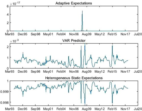Under the ${\mathcal{H}}_2$ predictor set (Figure 6), most firms (approximately 99.95%) use the Heterogeneous Static Expectation to form their inflation expectations. The proportions of the Adaptive Expectation and the VAR models are quite small. This shows that even though the cost of Heterogeneous Static Expectations is high, firms still willing to pay more to form more accurate inflation expectations. Thereby, firms’ inflation perceptions significantly affect their inflation expectations. Coibion and Gorodnichenko (2015) also find a strong correlation between corporates’ inflation perceptions and inflation expectations by studying the New Zealand firms.

Figure 5. The proportions of the Adaptive Expectation, VAR model, and the Rational Expectation for firms (November 1993 to June 2018). Source: Authors’ calculation.

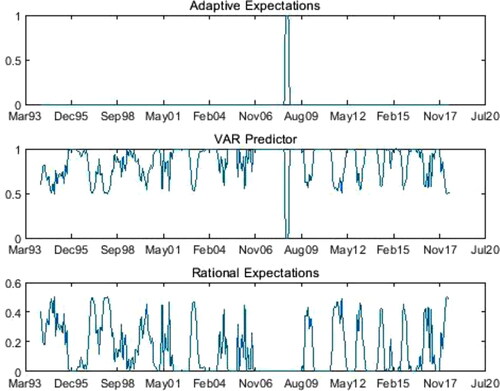
Figure 6. The proportions of the Adaptive Expectation, VAR model, and the Heterogeneous Static Expectation for firms (November 1993 to June 2018). Source: Authors’ calculation.

Figures 5 and 6 suggest that firms prefer to use the VAR predictor or the Heterogeneous Static Expectation to form inflation expectations, respectively. Figure 5 also shows that despite the costs of the VAR predictor and the Rational Expectation are high, there are more firms using the VAR model than the adaptive model. In other words, firms adopt more accurate predictors, i.e., VAR model and the Rational Expectation to form inflation expectations. Figure 6 provides further evidence which supports Coibion et al. (2018) that inflation perceptions is a non-negligible factor in forming inflation expectations. Besides, the results show that firms are not rational in forming inflation expectations. Thus, traditional macroeconomic models based on the Rational Expectation may generate certain deviations in investigating related problems of firms’ inflation expectations. Moreover, the micro-level inflation perceptions of firms have significant effects on the formation of their expectations. Thus, regulating the macro-economy through formulating monetary policies that aim to affect micro-inflation perceptions which influences firms’ inflation expectations provides possible useful policy tools.

5. Conclusion

Firms’ inflation expectations are the core of modern macroeconomic models, which determine the employment and pricing decisions. This paper investigates the novel inflation expectations of firms regarding the formation model and the heterogeneity between firms and households in forming inflation expectations. Focussing on the inflation expectation formation mechanisms, we find a significant heterogeneity between households and firms. Through investigating the possibility of agents in adopting a certain inflation expectation formation model, i.e., the proportion of a model being used by agents, the empirical tests suggest that firms’ inflation expectations are not perfectly rational. Amongst available inflation expectation formation models, firms prefer the Heterogeneous Static Expectation model over the VAR model, the Rational Expectation, the Adaptive Expectation, and the Naïve Expectation model. Thus, the firms’ inflation perception is a non-negligible factor in the formation of inflation expectations. This paper sheds lights on the central banks in regulating inflation expectations and the modelling of macro-economic problems.

Despite the research makes a comprehensive investigation regarding firms’ inflation expectations, there are several limitations. For example, because of data availability, this paper uses the survey of firms in the service sector, which causes the concern that the basket of products to which the expectations relate are not the same for firms and households. Additionally, the horizon of firms’ inflation expectations is 6 months, whereas it is 12 months for households. The above two aspects are possible sources of differences in the mechanisms of two groups in forming inflation expectations. Finding another way to measure firms’ inflation expectations for the future 12 months can solve the above problems. Unfortunately, current studies and surveys focus on expectations of households and professional forecasters, which thus leaves broad research prospects in the future.

Disclosure statement

No potential conflict of interest was reported by the authors.

Additional information

Funding

This work was supported by the National Natural Science Foundation of China [grant number 71873014]; the Fundamental Research Funds for the Central Universities, China [grant number FRF-BR-20-04B, QNXM20210048].

Notes

1 This statement can be found from the official files from FDSSSA at https://www.richmondfed.org/-/media/richmondfedorg/research/regional_economy/surveys_of_business_conditions/service_sector/errata/errata_service_sector_survey.pdf

2 According to Branch (2004), the qualitative results are robust to alternative choices of $\delta$ and lags. Hence, we refer to the selection of $\delta$ and lags according to the test results of Branch (2004) and make comparisons among various choices for robustness. The empirical results suggest that such specification provides the best fit of the data and we present the rounding off values of estimated results here for brevity.

References

- Bernanke, B., Reinhart, V., & Sack, B. (2004). Monetary policy alternatives at the zero bound: An empirical assessment. Brookings Papers on Economic Activity, 2004(2), 1–100. https://doi.org/10.1353/eca.2005.0002
- Bottone, M., & Rosolia, A. (2019). Monetary policy, firms’ inflation expectations and prices: causal evidence from firm-level data. Bank of Italy Temi di Discussione (Working Paper) No. 1218, This paper can be achieved at: https://ssrn.com/abstract=3432447
- Branch, W. A. (2004). The theory of rationally heterogeneous expectations: Evidence from survey data on inflation expectations. The Economic Journal, 114(497), 592–621. https://doi.org/10.1111/j.1468-0297.2004.00233.x
- Branch, W. A. (2007). Sticky information and model uncertainty in survey data on inflation expectations. Journal of Economic Dynamics and Control, 31(1), 245–276. https://doi.org/10.1016/j.jedc.2005.11.002
- Branch, W. A., & Evans, G. A. (2006). Simple recursive forecasting model. Economics Letters, 91(2), 158–166. https://doi.org/10.1016/j.econlet.2005.09.005
- Branch, W., & McGough, B. (2004). Multiple equilibria in heterogeneous expectations models. The B.E. Journal of Macroeconomics, 4(1), 1–16. https://doi.org/10.2202/1534-6005.1197
- Bräuning, C., & van der Cruijsen, C. (2019). Learning dynamics in the formation of European inflation expectations. Journal of Forecasting, 38(2), 122–135. https://doi.org/10.1002/for.2553
- Brock, W. A., & Hommes, C. H. (1997). A rational route to randomness. Econometrica: Journal of the Econometric Society, 65(5), 1059–1095. https://doi.org/10.2307/2171879
- Bryan, M. F., Meyer, B., & Parker, N. (2015). The inflation expectations of firms: What do they look like, are they accurate, and do they matter?. FRB Atlanta working paper https://doi.org/10.2139/ssrn.2580491
- Cagan, P. (1956). The monetary dynamics of hyperinflation. Studies in the Quantity Theory of Money This paper can be achieved at https://ci.nii.ac.jp/naid/10025285725/
- Coibion, O., & Gorodnichenko, Y. (2015). Is the Phillips curve alive and well after all? Inflation expectations and the missing disinflation. American Economic Journal: Macroeconomics, 7(1), 197–232. https://doi.org/10.1257/mac.20130306
- Coibion, O., Gorodnichenko, Y., & Kamdar, R. (2018). The formation of expectations, inflation, and the Phillips curve. Journal of Economic Literature, 56(4), 1447–1491. https://doi.org/10.1257/jel.20171300
- Dickey, D. A., & Fuller, W. A. (1981). Likelihood ratio statistics for autoregressive time series with a unit root. Econometrica, 49(4), 1057–1072. https://doi.org/10.2307/1912517
- Evans, G. W., & Honkapohja, S. (2012). Learning and expectations in macroeconomics. Princeton University Press.
- Ghosh, T., Sahu, S., & Chattopadhyay, S. (2020). Inflation expectations of households in India: Role of oil prices, economic policy uncertainty, and spillover of global financial uncertainty. Bulletin of Economic Research, 73(2), 230–251. https://doi.org/10.1111/boer.12244
- Gomez-Cram, R., & Yaron, A. (2021). How important are inflation expectations for the nominal yield curve? The Review of Financial Studies, 34(2), 985–1045. https://doi.org/10.1093/rfs/hhaa039
- Hubert, P., & Mirza, H. (2019). The role of forward‐ and backward‐looking information for inflation expectations formation. Journal of Forecasting, 38(8), 733–748. https://doi.org/10.1002/for.2596
- Kabundi, A., Schaling, E., & Some, M. (2015). Monetary policy and heterogeneous inflation expectations in South Africa. Economic Modelling, 45, 109–117. https://doi.org/10.1016/j.econmod.2014.11.002
- Kaihatsu, S., Shiraki,. Firms’ inflation expectations and wage-setting behaviors. Bank of Japan Working Paper, (2016). This paper can be achieved at: https://www.boj.or.jp/en/research/wps_rev/wps_2016/data/wp16e10.pdf
- Kitamura, T., Tanaka, M. Firms' inflation expectations under rational inattention and sticky information: an analysis with a small-scale macroeconomic model. Bank of Japan Working Paper Series, (2019). This paper can be achieved at: https://ideas.repec.org/p/boj/bojwps/wp19e16.html
- Lyziak, T. (2013). Formation of inflation expectations by different economic agents. Eastern European Economics, 51(6), 5–33. https://doi.org/10.2753/EEE0012-8775510601
- Lyziak, T. (2014). Inflation expectations in Poland, 2001-2013 measurement and macroeconomic testing. National Bank of Poland Working Paper, N0. 178.
- Lyziak, T. (2016). Do inflation expectations matter in a stylised New Keynesian model? The case of Poland. National Bank of Poland Working Paper, No. 234. This paper can be achieved at: https://ssrn.com/abstract=2804974
- Maag, T. (2010). Essays on inflation expectation formation [Doctoral dissertation, ETH Zurich]. https://doi.org/10.3929/ethz-a-006086165
- Mankiw, N. G., & Reis, R. (2002). Sticky information versus sticky prices: A proposal to replace the New Keynesian Phillips curve. The Quarterly Journal of Economics, 117(4), 1295–1328. https://doi.org/10.1162/003355302320935034
- Mankiw, N. G., Reis, R., & Wolfers, J. (2003). Disagreement about inflation expectations. NBER Macroeconomics Annual, 18, 209–248. This paper can be achieved at: https://doi.org/10.1086/ma.18.3585256
- Muth, J. F. (1961). Rational expectations and the theory of price movements. Econometrica, 29(3), 315–335. https://doi.org/10.2307/1909635
- Nakazono, J. K. Y. The formation of inflation expectations: micro-data evidence from Japan, Working Papers of Tokyo Center for Economic Research (2020). This paper can be achieved at: https://ideas.repec.org/p/tcr/wpaper/e144.html
- Nosratabadi, J. (2020). Do firms’ inflation expectations matter in their employment and wages? A causal evidence. SSRN Electronic Journal, This paper can be achieved at: https://ssrn.com/abstract=3575169
- Phillips, P. C. B., & Perron, P. (1988). Testing for a unit root in time series regression. Biometrika, 75(2), 335–346. https://doi.org/10.1093/biomet/75.2.335
- Pinto, S., Waddell, S., & Sarte, P. D. G. (2016). Monitoring economic activity in real time using diffusion indices: Evidence from the fifth district. Economic Quarterly, 101(04), 275–301. https://doi.org/10.21144/eq1010401
- Puah, C. H., Wong, S. S. L., & Habibullah, M. S. (2017). Are business forecasts of the construction sector rational? Survey-based evidence from Malaysia. Economic research-Ekonomska Istraživanja, 30(1), 858–872. https://doi.org/10.1080/1331677X.2017.1305794
- Rudd, J., & Whelan, K. (2007). Modeling inflation dynamics: A critical review of recent research. Journal of Money, Credit and Banking, 39, 155–170. https://doi.org/10.1111/j.1538-4616.2007.00019.x
- Schnorbus, R. H., & Watson, A. (2010). The service sector and the" great recession"-a fifth district perspective. The Federal Reserve Bank of Richmond working paper, No. 10-12,
- Sims, C. A. (2003). Implications of rational inattention. Journal of Monetary Economics, 50(3), 665–690. https://doi.org/10.1016/S0304-3932(03)00029-1
- Steindel, C., & Deitz, R. (2005). The Predictive Abilities of the New York Fed's Empire State Manufacturing Survey. Current Issues in Economics and Finance, 11(1), 1–7. This paper can be achieved at: https://www.newyorkfed.org/research/current_issues/ci11-1.html
- Uno, Y., Naganuma, S., Hara, N. New facts about firms' inflation expectations: simple tests for a sticky information model. Bank of Japan Working Paper Series, (2018). This paper can be achieved at: https://www.boj.or.jp/en/research/wps_rev/wps_2018/data/wp18e14.pdf
- Xu, Y., Chang, H. L., Lobonţ, O. R., & Su, C. W. (2016). Modeling heterogeneous inflation expectations: Empirical evidence from demographic data? Economic Modelling, 57, 153–163. https://doi.org/10.1016/j.econmod.2016.04.017
- Xu, H., Liu, H., Chen, T., Song, B., Zhu, J., Liu, X., Li, M., & Luo, C. (2021). Heterogeneous or homogeneous inflation expectation formation models: A case study of Chinese households and financial participants. Genes & Diseases, 8(5), 715–874. https://doi.org/10.1142/S0217590817400306