Volatility analysis based on GARCH-type models: Evidence from the Chinese stock market

Abstract

Volatility is integral for the financial market. As an emerging market, the Chinese stock market is acutely volatile. In this study, the data of the Shanghai Composite Index and Shenzhen Component Index returns were selected to conduct an empirical analysis based on the generalised autoregressive conditional heteroskedasticity (GARCH)-type model. We established the autoregressive moving average (ARMA)-GARCH model with t-distribution for the sample series to compare model effects under different distributions and orders. In contrast, we proposed threshold-GARCH (TGARCH) and exponential-GARCH (EGARCH) models to capture the features of the index. Additionally, the error degree and prediction results of different models were evaluated in terms of mean squared error (MSE), mean absolute error (MAE) and root-mean-squared error (RMSE). The results denote that the ARMA (4,4)-GARCH (1,1) model under Student’s t-distribution outperforms other models when forecasting the Shanghai Composite Index return series. For the return series of the Shenzhen Component Index, ARMA(1,1)-TGARCH(1,1) display the best forecasting performance among all models. This study could provide an effective information reference for the macro decision-making of the government, the operation of listed companies and investors’ investment decision-making.

Keywords:

• ARMA-GARCH
• GARCH
• stock markets
• volatility

JEL CODES:

• C22
• C52
• C53
• G10

1. Introduction

The Chinese stock market is an emerging market that attracts investors globally but is still in a nascent stage compared to its western counterparts. From the perspective of market operation characteristics, emerging markets have high turnover rates, high volatility and coexistence of high risk and high returns, showing strong speculation and instability. With regards to market standardisation, there are many problems in emerging markets, such as imperfect laws and regulations, inadequate law enforcement, and underdeveloped regulatory technology. Moreover, insider trading, stock market manipulation, and fraud are relatively common, and the degree of standardisation is not high. Emerging markets are usually dominated by individual investors, whose trading behaviour is often characterised by excessive trading, strong speculation, lack of rationality and long-term investment philosophy. Conversely, a mature stock market has a long history of development, and its legal system and market mechanisms are more optimised and reasonable. Institutional investors are also a vital constituent of a mature stock market, which is relatively more stable. Therefore, investors tend to be cautious of the volatility risk associated with emerging markets because of these differences between emerging and mature markets. Some scholars’ research may help investors understand the innovation and development capability of enterprises in emerging markets and provide crucial insights for the management’s investment decisions (Gil-Alana et al., 2020).

Emerging markets can promote the development of the economy, the horizontal financing of capital and the horizontal connection of the economy to enhance the overall efficiency of resource allocation. Besides, the scope of investment choices can be expanded to satisfy the diversified investment motives and interests of investors. Owing to uncertainty and high-speed international development, the Chinese stock market is experiencing a period characterised by both opportunities and risks. An accurate description of how stock prices fluctuate and how the future rate of stock market returns can be determined has become a pressing issue; hence, studying the volatility of the Chinese stock market is imperative.

2. Literature review

In the field of financial econometrics, the study of volatility in the financial market has garnered much attention. Bollerslev (1986) developed a model that encompasses the autoregressive conditional heteroscedasticity (ARCH) model, which he named the generalised autoregressive conditional heteroskedasticity (GARCH) model. The GARCH model has evolved into many GARCH-type models such as the exponential (EGARCH) model (Nelson, 1991), the GJR model (Glosten et al., 1993), and the periodic (PGARCH) model (Bollerslev & Ghysels, 1996). Even if the return series are significantly skewed (Gokcan, 2000), the GARCH model happens to be the most efficient tool for modelling. Engle (2002) introduces the GARCH extended (GARCH-X) model, which includes realised variance as an exogenous variable in the volatility dynamics equation. Ling and Li (2003) developed a limiting theory for unit root processes with GARCH disturbances. Berkes and Horváth (2004) introduced generalised non-Gaussian quasi-maximum likelihood (gQML) estimation of GARCH models. Wilhelmsson (2006) demonstrated the predictive power of the GARCH (1,1) model through returns from Standard & Poor’s (S&P) 500 index futures. To estimate the volatility of Taiwan Stock Index option prices, Tseng et al. (2008) integrated an EGARCH model and a feedforward neural network, whereas Xiao and Koenker (2009) studied the quantile regression for the linear GARCH model by utilising a truncated ARCH (∞) representation of volatilities.

Tan et al. (2010) implemented the wavelet tool in conjunction with the autoregressive integrated moving average (ARIMA) and the GARCH model to predict future prices accurately. Shephard and Sheppard (2010) proposed another extension of the GARCH-X model, called the high-frequency-based volatility (HEAVY) model. The multiplier methodology was extended to pseudo-observations by Rémillard (2012), including residuals of GARCH models. Klar et al. (2012) outlined that the specification of error distribution has a big impact on the efficiency of estimators despite having no effect on its asymptotic normality. The GARCH model with the error density approximated by the rational function with one parameter was found to fit the data better than the model with the Gaussian error density during the endeavour to find a rational approximation of the error density of the GARCH model (Chen & Takaishi, 2013; Takaishi & Chen, 2012). Li et al. (2014) characterise the asymptotic behaviours of volatilities in non-stationary GARCH (1,1) models. This characterisation provides more insight into the dynamics of volatilities in non-stationary GARCH models. Sun and Zhou (2014) denote how the tail index for GARCH models with a (1,1) lag structure can be calculated analytically for both the normal and Student’s t-conditional distribution assumptions. Hansen et al. (2014) developed a bivariate version of the realised GARCH to model the conditional variance and conditional beta of stock returns. Hansen et al. (2015) extended this process to the realised EGARCH model by employing a more flexible leverage function and enabling multiple realised measures. The model is extended to support a Constant Conditional Correlation (CCC)-GARCH structure and its usability was demonstrated by modelling and forecasting the return series comprising the Dow Jones Industrial Average (DJIA). Ismail, Audu, and Tumala (2016) have diligently applied their unique algorithm, the maximal overlap discreet wavelet transform (MODWT)-GARCH (1,1) model, and subsequently used it for comparisons with the performance of the traditional linear GARCH (1,1) model. Ismail et al. (2016) utilised the daily returns of four African countries’ stock market indices from January 2, 2000, to December 31, 2014. The authors found that the linear MODWT-GARCH (1,1) provides an accurate forecast value of the returns.

Narayan et al. (2016) put forward a GARCH (1,1) unit root model flexible enough to accommodate two endogenous structural breaks to test for unit roots among 156 US stocks listed on the New York Stock Exchange (NYSE) from 1980 to 2007. The mean recovery rate of most stocks was found to be better than that of non-stationary stock prices. Takaishi (2017) used a rational approximation for the volatility function in the GARCH model because it seemed to be a more promising approximation technique in comparison to the polynomial approximation used in other ARCH-type models. Realised GARCH models were applied by Jiang et al. (2018) to model the daily volatility of the E-mini S&P 500 index’s future returns. The authors confirmed that models using the generalised realised risk measures provide better volatility estimation for the in-sample, and that future volatility may be more attributable to present losses (i.e. risk measures). Gulzar et al. (2019) investigated the spillover effects of the global financial crisis on emerging Asian stock markets. Bivariate GARCH BEKK (Baba, Engle, Kraft, and Kroner) models confirmed the presence of spillover effects from the NYSE on emerging economies in all three cases (i.e. before, during and after the financial crisis). Milošević et al. (2019) used the ARCH and GARCH models to quantify the impact of the holiday effect on the rates of return from investing activities in the observed financial markets.

Using univariate asymmetric GARCH models, Aliyev et al. (2020) modelled and estimated the volatility of the Nasdaq-100 and found persistent volatility shocks on index returns, a leveraging effect on the index and asymmetric impact of shocks. Živkov et al. (2021) evaluated the multiscale bidirectional volatility spillover effect between national stocks and exchange rate markets among four African countries using the MS-GARCH model. Some scholars have also analysed the relationship between financial (i.e. gold returns) and social (i.e. worldwide Google attention on coronavirus) variables and the returns offered by the ESPO (the videogame and eSports exchange-traded fund). They revealed that the influence of social variables is weaker than that of financial variables (López-Cabarcos et al., 2020). Hongwiengjan and Thongtha (2021) assessed an analytical approximation of option prices using the TGARCH model. For empirical practice, a new efficient method for pricing options in the case of an in-the-money (ITM) option is provided. Kim et al. (2021) utilised the standard GARCH and various asymmetric GARCH models to compute the volatility of corporate bond yield spreads. Xu et al. (2021) proposed a novel quantile-based GARCH-MIDAS model to examine the influence of monthly economic policy uncertainty on the daily value-at-risk in the West Texas Intermediate crude oil spot and futures markets. Notably, a rise in eco-economic policy uncertainty was found to drive greater WTI crude oil market risk.

In the analysis of financial market volatility, previous researchers have applied many pioneering theories and methods, laying a solid foundation for later research. Primarily, scholars have used GARCH-type models to analyse the volatility of financial markets from different perspectives and determine the best model to describe characteristics of financial market volatility. Accordingly, this study analyses the fluctuation characteristics of the Chinese stock market. Investors need to better understand and grasp the operation law of the stock market and the fluctuation law of stock prices to reduce the blindness of investment. Such awareness will also help policymakers to better grasp the transmission mechanism of monetary policy and select and implement effective monetary policy.

The remainder of this paper is organised as follows. In Section 3, we briefly introduce the GARCH-type models used in this study. Section 4 contains the descriptive statistics of the samples, and Section 5 presents the results of the empirical analysis and the forecasting comparison of different estimation models. Lastly, the concluding remarks and implications are provided in Section 6.

3. Methodology

3.1. The ARMA model

The ARMA model, also known as the stationary time series model, is a combination of the AR and MA models. The basic expression is as follows: (1) $$y_t={\alpha }_0+\sum _{i=1}^p{\alpha }_i{y}_{t-i}+{\epsilon }_t+\sum _{i=1}^q{\beta }_i{\epsilon }_{t-i}$$(1)

$y_t$ represents the variable observed at period t, ${\epsilon }_{\mathrm{t}}$ is the independent error term, and $\alpha$ and $\beta$ are undetermined non-zero coefficients. The ARMA model can calculate variables influenced by both the past state and random factors existing in the present and the future. This characteristic makes the ARMA model suitable for research and prediction of long-term time series. The autoregression and trend of the time series can be easily deciphered by the ARMA model; however, it only performs well on stationary time series.

3.2. The ARCH model

The variance of a random variable is often assumed to be constant in traditional econometrics. In reality, financial time series have heteroscedasticity, which means that the data is stable in the long run, but unstable in the short term. To estimate the time variation, Engel proposed the ARCH model in 1982, which was used to model the mean and variance of sequences. The general expression of the ARCH model is as follows: (2) $$y_t=\varphi x_t+{\mu }_t$$(2) (3) $${\sigma }_{\mathrm{t}}^2=E({\mu }_{\mathrm{t}}^2|{\mu }_{t-1},{\mu }_{t-2}\dots )={\alpha }_0+{\alpha }_1{\mu }_{t-1}^2+\dots \dots +{\alpha }_p{\mu }_{t-p}^2=\sum _{i=1}^p{\alpha }_i{\mu }_{t-i}^2$$(3)

In the mean equation, $x_t$ is the independent variable observed in period t, $\varphi$ is a non-zero undetermined coefficient, and ${\mu }_{\mathrm{t}}$ is a random error term, which is assumed to follow a normal distribution in the general model. The basic principle of the ARCH model is that the variance of the residual sequence $\left\{{\mu }_t\right\}$ at time t is related to the square of the error term at time t-1. The ARCH model assumes that positive and negative volatility have the same impact on the response variable; hence, it cannot be employed to study series with asymmetric effects.

3.3. The GARCH model

Bollerslev (1986) proposed an important generalisation of the ARCH model, called the GARCH model, which can describe the tendency for volatility clustering in financial time series more precisely. Additionally, conditional variance is considered a GARCH process in this model to estimate time-varying volatility. The equations are defined as follows: (4) $$y_t=\varphi x_t+{\mu }_t,\mu \sim N(0,{\sigma }_t^2)$$(4) (5) $${\sigma }_t^2=\omega +\sum _{i=1}^p{\alpha }_i{\mu }_{t-i}^2+\sum _{i=1}^q{\beta }_i{\sigma }_{t-i}^2$$(5) where ${\mu }_{t-i}^2$ is the ARCH parameter, and ${\sigma }_{\mathrm{t}-\mathrm{i}}^2$ is the GARCH parameter. The coefficients of the ARCH and GARCH terms are denoted by $\alpha$ and $\beta ,$ respectively, and $p$ and $q$ are the lag order of the model. Thus, the ARCH model can be regarded as a special type of GARCH model. In the following research, we mainly undertake the GARCH-type model with one lag (i.e. GARCH (1,1) model) to estimate the sample series. The advantage of the GARCH model is that heteroscedasticity can be reflected and interpreted in the model; yet, it still fails to capture asymmetry.

3.4. The PARCH model

Taylor (1986) and Schwert (1989) proposed a standard deviation GARCH model. Compared with Bollerslev’s GARCH model, this model is used to fit the standard deviation to reduce the impact of large shocks on the conditional variance. Ding et al. (1993) further generalised the standard deviation GARCH model, naming it the power autoregressive conditional heteroscedasticity model (PARCH), with the following variance equation: (6) $${\sigma }_t^{\delta }=\omega +\sum _{j=1}^q{\beta }_j{\sigma }_{t-j}^{\delta }+\sum _{i=1}^p{\alpha }_i(|u_{t-i}|-{\gamma }_i{u}_{t-i}{)}^{\delta }$$(6) where $\delta$ is the power parameter of the estimated standard deviation, which is generally used to evaluate the magnitude of the impact on the conditional variance $\delta >0.$ $\gamma$ is an asymmetric coefficient that comprehends the asymmetric effect up to the order $r.$ When $i=1,2,\dots ,r,$ $\left|{\gamma }_i\right|\le 1,$ and when $i>r,$ ${\gamma }_i=0,r\le p.$ Compared with the GARCH model, the PARCH model cuts the restriction of non-negative parameters. The GARCH model cannot explain the negative correlation between the return on financial assets and the fluctuation of returns. As evident in Equation (5)(5) $${\sigma }_t^2=\omega +\sum _{i=1}^p{\alpha }_i{\mu }_{t-i}^2+\sum _{i=1}^q{\beta }_i{\sigma }_{t-i}^2$$(5) , the response of conditional variance to the change in positive and negative impacts is consistent, which is inconsistent with reality.

3.5. The component ARCH model

From the above subsection, we learn that the conditional variance GARCH (1,1) model is defined as: (7) $${\sigma }_t^2=\omega +\alpha \times u_{t-1}^2+\beta \times {\sigma }_{t-1}^2$$(7)

$\varpi$ is the long-term volatility. Assume$\omega =\varpi (1-\alpha -\beta )$ so that the equation can be obtained as: (8) $${\sigma }_t^2=\varpi +\alpha (u_{t-1}^2-\varpi )+\beta ({\sigma }_{t-1}^2-\varpi )$$(8)

The mean of the conditional variance in Equation (8)(8) $${\sigma }_t^2=\varpi +\alpha (u_{t-1}^2-\varpi )+\beta ({\sigma }_{t-1}^2-\varpi )$$(8) converges to a constant $\varpi .$ Subsequently, we replace $\varpi$ with a variable value $q_t,$ making it the equation for the component ARCH (CARCH) model: (9) $${\sigma }_t^2-q_t=\alpha (u_{t-1}^2-q_{t-1})+\beta ({\sigma }_{t-1}^2-q_{t-1})$$(9) (10) $$q_t=\omega +\rho (q_{t-1}-\omega )+\varphi (u_{t-1}^2-{\sigma }_{t-1}^2)$$(10)

The mean of the GARCH model is time-varying; in this case, $q_t$ is the long-term volatility changing over time. In Equation (9)(9) $${\sigma }_t^2-q_t=\alpha (u_{t-1}^2-q_{t-1})+\beta ({\sigma }_{t-1}^2-q_{t-1})$$(9) , the left side of the equation ${\sigma }_t^2-q_t$ is the short-term component, which converges to zero with action, while the left side in Equation (10)(10) $$q_t=\omega +\rho (q_{t-1}-\omega )+\varphi (u_{t-1}^2-{\sigma }_{t-1}^2)$$(10) represents the long-term component, which moves towards $\omega$ under the influence of the coefficient $\rho .$ The following equations are obtained when an asymmetric effect is introduced into the short-term equation: (11) $$q_t=\omega +\rho (q_{t-1}-\omega )+\varphi (u_{t-1}^2-{\sigma }_{t-1}^2)+{\theta }_1{z}_{1t}$$(11) (12) $${\sigma }_t^2-q_t=\alpha (u_{t-1}^2-q_{t-1})+\beta ({\sigma }_{t-1}^2-q_{t-1})+\gamma (u_{t-1}^2-q_{t-1})d_{t-1}+{\theta }_2{z}_{2t}$$(12) where $\rho ,$ $\varphi ,$ are $\theta$ non-zero undetermined coefficients, $z$ is an exogenous variable vector, $d_t$ is a dummy variable, and $\gamma$ is an asymmetric coefficient. When there is a positive impact, $u_{t-1}\ge 0,d_{t-1}=0.$ When a negative impact is observable, $u_{t-1}<0,d_{t-1}=1.$

3.6. The TGARCH model

Zakoian (1994) proposed the TGARCH model to further study the asymmetry of volatility. By introducing virtual variables into the original model, the following equation is obtained: (13) $$d_{t-1}=\{\begin{array}{cc}1,& {\mu }_{t-1}<0\\ 0,& {\mu }_{t-1}\ge 0\end{array}$$(13)

The TGARCH variance equation is defined as: (14) $${\sigma }_t^2=\omega +\sum _{i=1}^p{\alpha }_i{\mu }_{t-i}^2+\sum _{j=1}^q{\beta }_j{\sigma }_{t-j}^2+\sum _{k=1}^r{\gamma }_k{\mu }_{t-k}^2{d}_{t-k}$$(14)

Equation (14)(14) $${\sigma }_t^2=\omega +\sum _{i=1}^p{\alpha }_i{\mu }_{t-i}^2+\sum _{j=1}^q{\beta }_j{\sigma }_{t-j}^2+\sum _{k=1}^r{\gamma }_k{\mu }_{t-k}^2{d}_{t-k}$$(14) signifies that the value of ${\sigma }_t^2$ depends on that of the squared residual ${\mu }_{t-1}^2$ and the conditional variance of the previous period ${\sigma }_{t-1}^2.$ Furthermore, good and bad market news have different effects on the model. The asymmetric effect in the model is denoted by ${\gamma }_k{\mu }_{t-k}^2{d}_{t-k}.$ As long as the asymmetry coefficient $\gamma$ is not zero, there is an asymmetry in the time series. When negative news appears, ${\mu }_{t-1}<0$ and $d_{t-1}=1.$ When positive news emerges, ${\mu }_{t-1}\ge 0$ and $d_{t-1}=0.$ If $\gamma >0,$ there is a leverage effect in the sequence. However, if $\gamma <0,$ the asymmetric effect reduces volatility.

3.7. The EGARCH model

Nelson proposed the EGARCH model in 1991, providing the variance equation in logarithmic form. The EGARCH model is more convenient for estimating the parameters of ${\sigma }_t^2$ as it does not place any restrictions on the parameters of the model. (15) $$\text{ln}\hspace{0.17em}({\sigma }_t^2)=\omega +\sum _{i=1}^p{\alpha }_i\left|\frac{{\mu }_{t-i}}{{\sigma }_{t-i}}-E\left(\frac{{\mu }_{t-i}}{{\sigma }_{t-i}}\right)\right|+\sum _{j=1}^q{\beta }_j\hspace{0.17em}\text{ln}\hspace{0.17em}({\sigma }_{t-j}^2)+\sum _{k=1}^r{\gamma }_k\frac{{\mu }_{t-k}}{{\sigma }_{t-k}}$$(15)

${\sigma }_t^2$ is always positive regardless of whether the coefficient on the right side of Equation (15)(15) $$\text{ln}\hspace{0.17em}({\sigma }_t^2)=\omega +\sum _{i=1}^p{\alpha }_i\left|\frac{{\mu }_{t-i}}{{\sigma }_{t-i}}-E\left(\frac{{\mu }_{t-i}}{{\sigma }_{t-i}}\right)\right|+\sum _{j=1}^q{\beta }_j\hspace{0.17em}\text{ln}\hspace{0.17em}({\sigma }_{t-j}^2)+\sum _{k=1}^r{\gamma }_k\frac{{\mu }_{t-k}}{{\sigma }_{t-k}}$$(15) is positive or not. Therefore, compared with the GARCH model, the logarithmic conditional variance on the left side of the equation allows the coefficient to be negative, which makes the solution process more flexible. As long as there are unsymmetrical terms $\gamma \ne 0$ in the equation of the EGARCH model, its effect is measured by an exponential form rather than a quadratic form.

4. Descriptive statistics analysis

4.1. Data acquisition

The research was based on the daily closing prices of the Shanghai Composite Index and Shenzhen Component Index. Our dataset was obtained from the Guotai'an financial database, which contains data from 4 January 2000 to 4 March 2020. Each subsample covers 4885 trading days. The reasons for this dataset selection are as follows: first, the Shanghai Composite Index and the Shenzhen Component Index are representative stock indices in the Chinese stock market, which can reflect the overall performance and fluctuation pattern of stock prices. Second, the number of individual stocks during the initial stage (i.e. before 2000) of the Chinese stock market was rather small. A sample dataset covering this early period does not fulfil the requirements of the time series model. Furthermore, the daily price limit was not officially imposed in China until 1996. Hence, frequent abnormal fluctuations in the stock index in the previous period may affect the results of the model fitting. Third, most of the current studies concerning the volatility of the Chinese stock market are conducted with short time span data. Therefore, we decided to use a long time span sequence for modelling because the amount of time series data will impact the fitting results.

To better fit the model, log-returns of stock market index prices are used, as shown in Equation (16)(16) $$R_t=\hspace{0.17em}\text{ln}\hspace{0.17em}(p_t)-\hspace{0.17em}\text{ln}\hspace{0.17em}(p_{t-1})=\hspace{0.17em}\text{ln}\hspace{0.17em}\left(\frac{p_t}{p_{t-1}}\right)$$(16) : (16) $$R_t=\hspace{0.17em}\text{ln}\hspace{0.17em}(p_t)-\hspace{0.17em}\text{ln}\hspace{0.17em}(p_{t-1})=\hspace{0.17em}\text{ln}\hspace{0.17em}\left(\frac{p_t}{p_{t-1}}\right)$$(16) where $p_t$ is the closing price observed in period $t,$ $p_{t-1}$ is the daily closing price observed at period $t-1,$ and $R_t$ is the daily return of period $t.$ In the remainder of this paper, SH represents the Shanghai Composite Index return, and SCF represents the Shenzhen Component Index return.

4.2. Basic statistical analysis

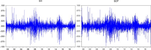
The two samples shown in Figure 1 have high volatility and large amplitude, and generally, display the characteristics of volatility clustering. Besides, Figure 1 exhibits three large-range volatilities experienced by the Chinese stock in the past 20 years, appearing in 2001–2002, 2006–2009 and 2014–2016. Among these durations, the volatility that occurred between 2006–2009 is exceptionally violent, with high returns and risks, but fluctuations in the other two durations are relatively small. Comparing the two plots, it is clear that SH and SCF share a similar trend; still, the volatility of the latter is more significant.

Figure 1. The daily indexes.

Source: statistical software EViews.

Figure 2 shown that the distributions of the SH and SCF return series are almost the same, demonstrating that the Shanghai and Shenzhen stock markets are highly correlated. The descriptive statistics depicted in Table 1 show that the mean returns of both samples are positive and close to zero, while the SCF series portrays a relatively higher level of return. Additionally, the standard deviation value of SH is 0.0156, and that of SCF is 0.0176, implying that the risk level of the Shanghai stock market is lower than that of the Shenzhen stock market and that the former market is more stable than the latter.

Figure 2. Descriptive statistics of index returns.

Source: statistical software EViews.

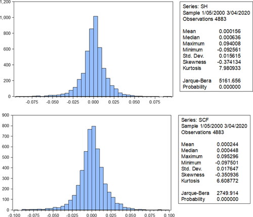
Table 1. Descriptive statistics.

	Sample Size	Mean	Std.	Skewness	Kurtosis	J–B Statistics	P-value
SH	4883	0.000156	0.0156	−0.3741	7.9809	5161.656	0.0000
SCF	4883	0.000244	0.0176	−0.3509	6.6087	2749.914	0.0000

Source: statistical results.

The p-values of the J–B normality test for the two return series are both 0, confirming that the null hypothesis of normality is rejected at the 5% level of significance, and the return series of the SH and the SCF are not normally distributed. Likewise, the skewness of the two series is negative and close to 0, and kurtosis is greater than 3, verifying that the return of the Chinese stock market is leptokurtic and thick-tailed. Moreover, the SCF has a smaller degree of skewness than the SH; thus, we can assume that the distribution of the SH return series is more imbalanced.

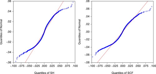
Figure 3 displays the Q-Q plots of the SH and the SCF series. The presence of scattered points deviating from normal distribution at both the left end and the right tail is a strong confirmation of the findings obtained and displayed above.

Figure 3. Q-Q plots of return series.

Source: statistical software EViews.

Through the above descriptive statistical analysis, we found that the return series of Shanghai and Shenzhen stock markets show characteristics of volatility clusters, peaks and fat tails. The return series of SH and SCF are highly similar, which indicates that there is a strong correlation between the Shanghai and Shenzhen stock markets, and neither of them follows a normal distribution. The risk level of the Shanghai and Shenzhen stock markets is lower from the perspective of volatility risk, however, the former is more stable than the latter.

4.3. Preparation before modelling

Pre-processing of the time series is required before modelling. The stationarity of the sequence must be confirmed to avoid spurious regression in model estimation. Subsequently, we need to find the optimal lag order of the ARMA (p,q) model through an autocorrelation test to attain the best fitting results. Finally, the GARCH model’s validity is affirmed by testing the ARCH effect of the sequence.

4.3.1. Unit root test

The Augmented Dickey–Fuller (ADF) test method is employed to test the return series of SH and SCF, and the outcomes are presented in Table 2. The findings prove that the t-statistics of the two series are far less than critical values at the 1%, 5% or 10% significance levels, outlining that there is no unit root in the sample series, and they are stationary time series.

Table 9. Summary statistics in SCF.

	SCF-GARCH	AIC	SC	Mean
Normal distribution	GARCH (1,1)	−5.468396	−5.461746	−5.465071
	GARCH (1, 2)	−5.467996	−5.460016	−5.464006
	GARCH (2,1)	−5.466064	−5.458084	−5.462074
Student’s t-distribution	GARCH (1,1)	−5.530729	−5.522748	−5.5267385
	GARCH (1, 2)	−5.53053	−5.521219	−5.5258745
	GARCH (2,1)	−5.526506	−5.517196	−5.521851
Generalised error distribution	GARCH (1,1)	−5.52948	−5.5215	−5.52549
	GARCH (1, 2)	−5.529154	−5.519844	−5.524499
	GARCH (2,1)	−5.52922	−5.51991	−5.524565

Source: statistical results.

Table 2. ADF test results.

	T-statistics	The Significance Level of 1%	The Significance Level of 5%	The Significance Level of 10%	P-value
SH	−68.3937	−3.4315	−2.8619	−2.5670	0.0001
SCF	−66.7596	−3.4315	−2.8619	−2.5670	0.0001

Source: statistical results.

4.3.2. Autocorrelation test

In this subsection, Ljung–Box Q (LBQ) statistics, autocorrelation (AC) graph, and partial autocorrelation (PAC) graph are utilised to determine the optimal lag order of the ARMA model. The area between the dotted lines in Table 3 is twice the estimated standard deviation, and the grey area depicts the AC and PAC coefficients of the return series. We can conclude that there is no significant difference between the coefficients and 0 at the 5% significance level provided these coefficients lie between the dotted lines. If they are beyond the dotted line, there is autocorrelation in the return series.

Table 3. The autocorrelation test results in SH.

Autocorrelation	Partial Autocorrelation		AC	PAC	Q-statistics	P-value
		1	0.021	0.021	2.1861	0.139
		2	−0.022	−0.022	4.5307	0.104
		3	0.028	0.029	8.2587	0.041
		4	0.048	0.047	19.684	0.001
		5	−0.004	−0.005	19.771	0.001
		6	−0.051	−0.050	32.638	0.000
		7	0.031	0.031	37.358	0.000
		8	0.009	0.004	37.758	0.000
		9	0.004	0.008	37.830	0.000
		10	−0.002	0.002	37.842	0.000

Source: statistical results.

Tables 3 and 4 verify that the AC and PAC coefficients of the two return series fluctuate around 0, which can be ignored. The probability value of SH is less than 5% after the lag order is greater than 3, while the probability value of SCF is always less than 5%. Therefore, both return series have significant autocorrelation.

Table 10. Estimation for ARMA (4,4)-GARCH (1,1) in SH.

SH	Variables	Coefficient	Std.	Z-statistics	P-value
Mean equation	AR (1(1) $$y_t={\alpha }_0+\sum _{i=1}^p{\alpha }_i{y}_{t-i}+{\epsilon }_t+\sum _{i=1}^q{\beta }_i{\epsilon }_{t-i}$$(1) )	0.677042	0.382763	1.768827	0.0769
(ARMA)	AR (2(2) $$y_t=\varphi x_t+{\mu }_t$$(2) )	0.124923	0.258004	0.484192	0.6282
	AR (3(3) $${\sigma }_{\mathrm{t}}^2=E({\mu }_{\mathrm{t}}^2|{\mu }_{t-1},{\mu }_{t-2}\dots )={\alpha }_0+{\alpha }_1{\mu }_{t-1}^2+\dots \dots +{\alpha }_p{\mu }_{t-p}^2=\sum _{i=1}^p{\alpha }_i{\mu }_{t-i}^2$$(3) )	−0.550004	0.216142	−2.544645	0.0109
	AR (4(4) $$y_t=\varphi x_t+{\mu }_t,\mu \sim N(0,{\sigma }_t^2)$$(4) )	0.134562	0.256962	0.523665	0.6005
	MA (1(1) $$y_t={\alpha }_0+\sum _{i=1}^p{\alpha }_i{y}_{t-i}+{\epsilon }_t+\sum _{i=1}^q{\beta }_i{\epsilon }_{t-i}$$(1) )	−0.662400	0.381017	−1.738506	0.0821
	MA (2(2) $$y_t=\varphi x_t+{\mu }_t$$(2) )	0.128068	0.248170	−0.516050	0.6058
	MA (3(3) $${\sigma }_{\mathrm{t}}^2=E({\mu }_{\mathrm{t}}^2|{\mu }_{t-1},{\mu }_{t-2}\dots )={\alpha }_0+{\alpha }_1{\mu }_{t-1}^2+\dots \dots +{\alpha }_p{\mu }_{t-p}^2=\sum _{i=1}^p{\alpha }_i{\mu }_{t-i}^2$$(3) )	0.583425	0.208923	2.792540	0.0052
	MA (4(4) $$y_t=\varphi x_t+{\mu }_t,\mu \sim N(0,{\sigma }_t^2)$$(4) )	−0.165291	0.261328	−0.632503	0.5271
Variance equation	$\omega$	1.25E-06	3.59E-07	3.497888	0.0005
(GARCH)	ARCH parameter	0.064365	0.004988	9.210643	0.0000
	GARCH parameter	0.935054	0.006344	147.3881	0.0000

Source: statistical results.

Table 11. Estimation for ARMA (1,1)-GARCH (1,1) in SCF.

SCF	Variables	Coefficient	Std.	Z-statistics	P-value
Mean equation	AR (1(1) $$y_t={\alpha }_0+\sum _{i=1}^p{\alpha }_i{y}_{t-i}+{\epsilon }_t+\sum _{i=1}^q{\beta }_i{\epsilon }_{t-i}$$(1) )	−0.777718	0.156431	−4.971648	0.0000
(ARMA)	MA (1(1) $$y_t={\alpha }_0+\sum _{i=1}^p{\alpha }_i{y}_{t-i}+{\epsilon }_t+\sum _{i=1}^q{\beta }_i{\epsilon }_{t-i}$$(1) )	0.798818	0.149967	5.326618	0.0000
Variance equation	$\omega$	2.95E-06	7.13E-07	4.137136	0.0000
(GARCH)	ARCH parameter	0.066557	0.007421	8.969182	0.0000
	GARCH parameter	0.926246	0.007579	122.2111	0.0000

Source: statistical results.

Table 3 exhibits that the correlation coefficients of the SH series are relatively significant when the lag order is 4 or 6. Thus, we established four models for the SH series, namely ARMA (4,4), ARMA (4,6), ARMA (6,4), and ARMA (6,6). Table 4 provides the correlation coefficients of the SCF series, which are significant at lags 1 and 7. Moreover, four models are established based on ARMA (1,1), ARMA (1,7), ARMA (7,1), and ARMA (7,7).

Table 4. The autocorrelation test results in SCF.

Autocorrelation	Partial Autocorrelation		AC	PAC	Q-statistics	P-value
		1	0.045	0.045	10.038	0.002
		2	−0.023	−0.025	12.598	0.002
		3	0.028	0.030	16.429	0.001
		4	0.034	0.030	21.970	0.000
		5	−0.007	−0.009	22.222	0.000
		6	−0.025	−0.024	25.348	0.000
		7	0.042	0.043	34.095	0.000
		8	0.011	0.005	34.666	0.000
		9	0.001	0.005	34.675	0.000
		10	−0.004	−0.004	34.742	0.000

Source: statistical results.

The lag order was related to the reliability of the model. Improper selection of lag order results in the omission of relevant information accommodation. Table 5 illustrates the estimation results of the different ARMA models. We employed ARMA (4,4) to approximate the SH return series and ARMA (1,1) to compute the SCF return series based on the Akaike information criterion (AIC) and Schwarz criterion (SC).

Table 5. ARMA model estimation results of SH and SCF return series.

SH	AIC	SC	Mean
ARMA (4,4)	−5.4893	−5.4787	−5.4840
ARMA (4, 6)	−5.4899	−5.4766	−5.4833
ARMA (6,4)	−5.4887	−5.4783	−5.4835
ARMA (6,6)	−5.4885	−5.4725	−5.4805
SH	AIC	SC	Mean
ARMA (1,1)	−5.2388	−5.2362	−5.2375
ARMA (1, 7)	−5.2410	−5.2304	−5.2357
ARMA (7,1)	−5.2427	−5.2313	−5.2370
ARMA (7,7)	−5.2450	−5.2263	−5.2356

Source: statistical results.

4.3.3. The test of ARCH effect

The Shanghai and Shenzhen stock markets exhibit the characteristics of volatility clustering, signifying that two return series may have an ARCH effect. We investigated the ARCH effect of two return series to measure heteroscedasticity more accurately. A test was used for the correlogram of squared residuals based on the LBQ statistics.

Q-Statistics are considered in Tables 6 and 7 for detecting autocorrelation and are associated with probability values. The null hypothesis is rejected if the probability value is less than 0.05, and the sequence has autocorrelation. The test results of Q-statistics in the table above confirms that the probability p-values are all less than 5%, signalling that the two squared residual series have autocorrelation, and the SH and SCF return series have a significant ARCH effect.

Table 13. Estimation for PARCH (1,1) in SH.

SH	Variables	Coefficient	Std.	Z-statistics	P-value
Variance equation	$\omega$	9.81E-05	8.01E-05	1.223889	0.2210
(PARCH)	$\alpha$	0.080390	0.007609	10.56515	0.0000
	$\gamma$	0.183320	0.054283	3.377141	0.0007
	$\beta$	0.933875	0.006341	147.2709	0.0000
	$\delta$	0.044826	0.179298	5.827307	0.0000

Source: statistical results.

Table 14. Estimation for PARCH (1,1) in SCF.

SCF	Variables	Coefficient	Std.	Z-statistics	P-value
Variance equation	$\omega$	0.000253	0.000200	1.266037	0.2055
(PARCH)	$\alpha$	0.079024	0.007573	10.43472	0.0000
	$\gamma$	0.201582	0.054292	3.712925	0.0002
	$\beta$	0.930792	0.006829	136.3005	0.0000
	$\delta$	0.922191	0.181949	5.068395	0.0000

Source: statistical results.

Some preparations are introduced before the modelling procedure in Section 4.3. First, we test the stationarity of time-series data and certify that the revenue series of SH and SCF are stationary. Then, the optimal lag order of the ARMA (p, q) model is determined by an autocorrelation test. Based on the AIC and SC criteria, we find that the ARMA (4,4) and ARMA (1,1) models are best for estimating the return series of SH and SCF. Lastly, we conclude that the SH and SCF return series have a significant ARCH effect by testing the squared residual correlation graph of the LBQ statistic.

5. Empirical analysis

5.1. Garch model selection

GARCH (1,1), GARCH (1, 2) and GARCH (2, 1) were established for the SH and SCF sample data, respectively. The fitting results were compared and the most suitable model was selected for the return time series under normal distribution, Student’s t-distribution and generalised error distribution. The estimation results of empirical analysis in this section are given in Tables 8-28 in the Appendix.

Table 8. Summary statistics in SH.

	SH-GARCH	AIC	SC	Mean
Normal distribution	GARCH (1,1)	−5.775053	−5.760415	−5.767734
	GARCH (1, 2)	−5.774783	−5.758814	−5.7667985
	GARCH (2,1)	−5.773185	−5.757216	−5.7652005
Student’s t-distribution	GARCH (1,1)	−5.859664	−5.843695	−5.8516795
	GARCH (1, 2)	−5.859736	−5.842437	−5.8510865
	GARCH (2,1)	−5.860116	−5.842817	−5.8514665
Generalised error distribution	GARCH (1,1)	−5.859201	−5.843233	−5.851217
	GARCH (1, 2)	−5.858948	−5.841648	−5.850298
	GARCH (2,1)	−5.859036	−5.841736	−5.850386

Source: statistical results.

Table 15. Results of the ARCH-LM test for the PARCH model.

	F-statistics	Probability	$T\times R^2$ Statistics	Probability
SH	0.726645	0.3940	0.726834	0.3939
SCF	0.289720	0.5904	0.289822	0.5903

Source: statistical results.

Table 16. Estimation results of CARCH (1,1) for SH.

SH	Variables	Coefficient	Std.	Z-statistics	P-value
Variance equation	$\omega$	0.004638	0.011617	0.399226	0.6897
(CARCH)	$\rho$	0.999722	0.000710	1407.496	0.0000
	$\varphi$	0.068794	0.006517	10.55607	0.0000
	$\alpha$	−0.062890	0.020310	−3.096562	0.0020
	$\gamma$	0.073117	0.028678	2.549594	0.0108
	$\beta$	0.640358	0.196195	3.263879	0.0011

Source: statistical results.

Table 17. Estimation results of CARCH (1,1) for SCF.

SCF	Variables	Coefficient	Std.	Z-statistics	P-value
Variance equation	$\omega$	0.000412	0.000173	2.386235	0.0170
(CARCH)	$\rho$	0.992354	0.004110	241.4322	0.0000
	$\varphi$	0.069251	0.007643	9.060927	0.0000
	$\alpha$	−0.039013	0.024711	−1.578804	0.1144
	$\gamma$	0.014143	0.032789	0.431318	0.6662
	$\beta$	−0.232817	0.561740	−0.414458	0.6785

Source: statistical results.

Table 18. Results of the ARCH-LM test for the CARCH model.

	F-statistics	Probability	$T\times R^2$ Statistics	Probability
SH	1.520640	0.2176	1.520790	0.2175
SCF	1.997023	0.1577	1.997024	0.1576

Source: statistical results.

Table 19. Estimation results of TGARCH (1,1) for SH.

SH	Variables	Coefficient	Std.	Z-statistics	P-value
Variance equation	$\omega$	1.44E-06	3.81E-07	3.770795	0.0002
(TGARCH)	$\alpha$	0.052649	0.008181	6.435696	0.0000
	$\lambda$	0.028738	0.010537	2.727310	0.0064
	$\beta$	0.931614	0.006491	143.5330	0.0000

Source: statistical results.

Table 20. Estimation results of TGARCH (1,1) for SCF.

SCF	Variables	Coefficient	Std.	Z-statistics	P-value
Variance equation	$\omega$	3.23E-06	7.40E-07	4.362482	0.0000
(TGARCH)	$\alpha$	0.050050	0.008197	6.105689	0.0000
	$\lambda$	0.036598	0.010735	3.409107	0.0007
	$\beta$	0.923446	0.007620	121.1859	0.0000

Source: statistical results.

Table 21. Results of the ARCH-LM test for the TGARCH model.

	F-statistics	Probability	$T\times R^2$ Statistics	Probability
SH	0.532270	0.7120	2.130335	0.7118
SCF	0.094907	0.7580	0.094944	0.7580

Source: statistical results.

Table 22. Estimates of EGARCH (1,1) for SH.

SH	Variables	Coefficient	Std.	Z-statistics	P-value
Variance equation	$\omega$	−0.194159	0.025892	−7.498868	0.0000
(EGARCH)	$\alpha$	0.153050	0.013938	10.98043	0.0000
	$\lambda$	−0.028658	0.007799	−3.674773	0.0002
	$\beta$	0.990301	0.002467	401.4211	0.0000

Source: statistical results.

Table 23. Estimates of EGARCH (1,1) for SCF.

SCF	Variables	Coefficient	Std.	Z-statistics	P-value
Variance equation	$\omega$	−0.207422	0.027986	−7.411757	0.0000
(EGARCH)	$\alpha$	0.150245	0.013806	10.88240	0.0000
	$\lambda$	−0.028715	0.007515	−3.821092	0.0001
	$\beta$	0.988419	0.002804	352.5051	0.0000

Source: statistical results.

Table 24. Results of the ARCH-LM test for the EGARCH model.

	F-statistics	Probability	$T\times R^2$ Statistics	Probability
SH	0.975060	0.4198	3.901122	0.4196
SCF	0.236844	0.6265	0.236929	0.6264

Source: statistical results.

Table 25. Forecast values of the SH series.

Date	Real Return	GARCH (1,1)	TGARCH (1,1)	EGARCH (1,1)	PARCH (1,1)	CARCH (1,1)
2020-03-05	−0.012173	0.002141	0.002155	0.001054	0.001337	0.001316
2020-03-06	−0.030522	0.000218	0.000264	0.001264	0.000604	0.000438
2020-03-09	0.018004	0.000934	0.001006	0.000544	0.000920	0.000811
2020-03-10	−0.009470	−0.000839	−0.000803	−0.000406	−0.000764	−0.000807
2020-03-11	−0.015286	−0.000284	−0.000248	−0.000486	−0.000160	−0.000092
2020-03-12	−0.012411	−0.000781	−0.000777	−0.000134	−0.000239	−0.000186
2020-03-13	−0.034592	0.000023	0.000042	0.000229	0.000543	0.000563
2020-03-16	−0.003452	−0.000039	−0.000044	0.000161	−0.000023	−0.000071
2020-03-17	−0.018476	0.000368	0.000369	0.000026	0.000022	−0.000015
2020-03-18	−0.009805	0.000126	0.000105	−0.000118	−0.000297	−0.000301

Source: statistical results.

Table 26. Forecast values of the SCF series.

Date	Real Return	ARMA (1,1)- GARCH (1,1)	ARMA (1,1)- TGARCH (1,1)	ARMA (1,1)- EGARCH (1,1)	ARMA (1,1)- PARCH (1,1)	ARMA (1,1)- CARCH (1,1)
2020-03-05	−0.011038	0.001045	0.001110	0.001074	0.001051	0.000991
2020-03-06	−0.041808	−0.000813	−0.000861	−0.000834	−0.000814	−0.000781
2020-03-09	0.026203	0.000632	0.000667	0.000647	0.000631	0.000615
2020-03-10	−0.017999	−0.000492	−0.000517	−0.000502	−0.000489	−0.000484
2020-03-11	−0.023400	0.000382	0.000401	0.000390	0.000379	0.000381
2020-03-12	−0.010094	−0.000297	−0.000311	−0.000303	−0.000293	−0.000300
2020-03-13	−0.054826	0.000231	0.000241	0.000235	0.000227	0.000237
2020-03-16	−0.004941	−0.000180	−0.000187	−0.000182	−0.000176	−0.000186
2020-03-17	−0.017120	0.000140	0.000145	0.000141	0.000136	0.000147
2020-03-18	−0.000969	−0.000109	−0.000112	−0.000110	−0.000106	−0.000116

Source: statistical results.

Table 27. Loss function values of the forecasting of SH return series.

	ARMA (4,4)- GARCH (1,1)	ARMA (4,4)- TGARCH (1,1)	ARMA (4,4)- EGARCH (1,1)	ARMA (4,4)- PARCH (1,1)	ARMA (4,4)- CARCH (1,1)
MSE	0.000354	0.000354	0.000360	0.000357	0.000357
MAE	0.016419	0.016425	0.016524	0.016429	0.016423
RMSE	0.018814	0.018823	0.018984	0.018907	0.018894
MEAN	0.011862	0.011867	0.011956	0.011898	0.011891

Source: statistical results.

Table 28. Loss function values of the forecasting of SCF return series.

	ARMA (1,1)- GARCH (1,1)	ARMA (1,1)- TGARCH (1,1)	ARMA (1,1)- EGARCH (1,1)	ARMA (1,1)- PARCH (1,1)	ARMA (1,1)- CARCH (1,1)
MSE	0.000680	0.000680	0.000680	0.000680	0.000680
MAE	0.020767	0.020764	0.020766	0.020768	0.020767
RMSE	0.026079	0.026073	0.026076	0.026078	0.026085
MEAN	0.015842	0.015839	0.015841	0.015842	0.015844

Source: statistical results.

Table 6. The autocorrelation test results of SH’s squared residual.

Autocorrelation	Partial Autocorrelation		AC	PAC	Q-statistics	P-value
		1	0.160	0.160	124.52	0.000
		2	0.141	0.119	221.83	0.000
		3	0.180	0.147	380.18	0.000
		4	0.151	0.098	492.11	0.000
		5	0.130	0.068	574.76	0.000
		6	0.120	0.051	644.76	0.000
		7	0.131	0.064	729.12	0.000
		8	0.119	0.048	798.73	0.000
		9	0.090	0.016	838.09	0.000
		10	0.146	0.081	942.65	0.000

Source: statistical results.

Table 7. The autocorrelation test results of SCF’s squared residual.

Autocorrelation	Partial Autocorrelation		AC	PAC	Q-statistics	P-value
		1	0.152	0.152	112.70	0.000
		2	0.168	0.148	250.80	0.000
		3	0.173	0.134	396.31	0.000
		4	0.157	0.102	516.67	0.000
		5	0.127	0.060	595.90	0.000
		6	0.128	0.058	676.05	0.000
		7	0.138	0.069	769.67	0.000
		8	0.148	0.076	876.71	0.000
		9	0.091	0.009	917.53	0.000
		10	0.150	0.075	1027.1	0.000

Source: statistical results.

According to the values of AIC and SC, the GARCH (1,1) model with the Student’s t-distribution is the most suitable model for the SH and SCF samples. Therefore, we establish ARMA (4,4)-GARCH (1,1) with the Student’s t-distribution to estimate the SH return series, and ARMA (1,1)-GARCH (1,1) with the Student’s t-distribution to compute the SCF return series.

5.2. Estimation results

The findings acquired by EViews 8.0 are expressed in Tables 10 and 11. The variance equation of the GARCH (1,1) model for the SH is as follows: (17) $${\sigma }_t^2=1.25\times {10}^{-6}+0.0644{\mu }_{t-1}^2+0.935{\sigma }_{t-1}^2$$(17)

The variance equation of the GARCH (1) model for SCF is expressed as: (18) $${\sigma }_t^2=2.95\times {10}^{-6}+0.0666{\mu }_{t-1}^2+0.9262{\sigma }_{t-1}^2$$(18)

We can observe from the estimation outcomes that the coefficients, the p-values of the ARCH and GARCH terms are all close to 0, verifying that the model fits well at the 1% significance level.

Second, the results of the ARCH-LM test for sequence residuals are presented in Table 12. The F-statistic reveals the joint significance of the squares of residuals for all lag orders. The $T\times R^2$ statistic represents the product of the sample sizes $T$ and $R^2.$ The p-values are all greater than 0.05, allowing us to accept the null hypothesis. This evidence substantiates the applicability of the GARCH (1,1), and that the ARCH effect is eliminated.

Table 12. Results of ARCH-LM test.

	F-statistics	Probability	$T\times R^2$ Statistics	Probability
SH	0.829600	0.5061	3.319546	0.5058
SCF	0.053695	0.8168	0.053716	0.8167

Source: statistical results.

For the SH series, the sum of the GARCH and ARCH parameters was 0.9994, and the sum of the two parameters was 0.9928 in the case of the SCF sequence. Both numbers are less than but close to 1, satisfying the constraint condition of the parameter and highlighting that the impact of the volatility is continuous but may weaken over time.

Overall, the GARCH (1,1) model with Student’s t-distribution outperforms other models in capturing the volatility of the Chinese stock market, but it cannot be employed to explain the asymmetric effect of the stock market because of the limitation of the model itself. Therefore, in the next two subsections, we use the TGARCH and EGARCH models to further elucidate the volatility characteristics of the Chinese stock market.

5.3. Estimation analysis based on PARCH model

We established the power ARCH (1,1) model to estimate the sample series. The outcomes are displayed in Tables 13 and 14, where the variance equation of the SH series can be obtained as follows: (19) $${\sigma }_t^{1.045}=9.81\times {10}^{-5}+0.08{(\left|u_{t-1}\right|-0.183u_{t-1})}^{1.045}+0.934{\sigma }_{t-1}^{1.045}$$(19)

The estimated variance equation for the SCF sequence is: (20) $${\sigma }_t^{0.922}=2.53\times {10}^{-4}+0.079{(\left|u_{t-1}\right|-0.202u_{t-1})}^{0.922}+0.931{\sigma }_{t-1}^{0.922}$$(20)

According to the p-values of the coefficients in Table 15 and the ARCH-LM test results, heteroscedasticity was eliminated. Thus, this model can explain the asymmetry of the Shanghai and Shenzhen stock markets. From the results of the equation, the asymmetric coefficient is 0.0183 in SH and 0.202 in SCF, establishing the existence of the “leverage effect”. This effect is more potent on the Shenzhen Component Index than on Shanghai Composite Index and outlines that when the Chinese stock market is subjected to the same bad news, the price fluctuation response of the Shenzhen Component Index is greater than that of the Shanghai Composite Index.

5.4. Estimation analysis based on the CARCH model

In this subsection, we use the asymmetric CARCH (1,1). The findings are outlined in Tables 16 and 17. The variance equation for the SH sequence can be obtained as follows.

Short term equation: (21) $$q_t=4.638\times {10}^{-3}+0.9997(q_{t-1}-4.638\times {10}^{-3})+0.688(u_{t-1}^2-{\sigma }_{t-1}^2)$$(21)

Long term equation: (22) $${\sigma }_t^2-q_t=0.64({\sigma }_{t-1}^2-q_{t-1})+(0.0731d_{t-1}-0.0629)(u_{t-1}^2-q_{t-1})$$(22)

The short-term equation estimated from the SCF sequence: (23) $$q_t=4.12\times {10}^{-4}+0.992(q_{t-1}-4.12\times {10}^{-4})+0.0693(u_{t-1}^2-{\sigma }_{t-1}^2)$$(23)

The long-term equation: (24) $${\sigma }_t^2-q_t=-0.2328({\sigma }_{t-1}^2-q_{t-1})+(0.0141d_{t-1}-0.039)(u_{t-1}^2-q_{t-1})$$(24)

Table 18 exemplifies that the significant p-values are all greater than 0.05; hence, the CARCH model has an excellent fitting performance. Besides, the asymmetric coefficients of the SH and SCF equations were 0.0731 and 0.01414, respectively. We can conclude that the negative shock is larger than the positive shock in the SH and SCF series because the dummy variable in CARCH denotes the negative shock, and the asymmetry effect is transient from the estimation results. Additionally, the long-term volatility of the two sequences converged slowly at a similar rate.

5.5. Estimation based on the TGARCH model

As proposed in the second section, we introduce a dummy variable into the GARCH model and determine the TGARCH (1,1) model with the Student’s t-distribution. The estimation results are provided in Tables 19 and 20, and the variance equation of the SH sequence is expressed as: (25) $${\sigma }_t^2=1.44\times {10}^{-6}+0.0526{\mu }_{t-1}^2+0.0287{\mu }_{t-1}^2{d}_{t-1}+0.9316{\sigma }_{t-1}^2$$(25)

The variance equation for the SCF sequence is expressed as: (26) $${\sigma }_t^2=3.23\times {10}^{-6}+0.05{\mu }_{t-1}^2+0.0366{\mu }_{t-1}^2{d}_{t-1}+0.9234{\sigma }_{t-1}^2$$(26)

Tables 19 and 20 illustrate that the p-values of the equation coefficients are close to 0, suggesting that the model excels in capturing volatility. Moreover, the ARCH-LM test in Table 21 authenticates that the p-value of the F-statistic and $T\times R^2$ statistic is greater than 0.05, proving the applicability of the TGARCH (1,1) model.

Correspondingly, we discovered that the coefficients of the asymmetric parameter are 0.0287 and 0.0366, respectively, which reveals the presence of the “leverage effect” in the Chinese market. Additionally, the coefficients are all positive, indicating that good news exerts a more substantial effect on the market than bad news.

In terms of the parameters of the model, the outcome of the SH series reveals that positive news will impact $\alpha =0.0526$ times on returns, while negative news will bring $\gamma +\alpha =0.0526+0.0287=0.0813$ times the impact. As for the SCF series, the impact brought by good news is $\alpha =0.05$ times, and that of bad news is $\gamma +\alpha =0.05+0.0366=0.0866$ times. These statistics corroborate that the volatility of the Shanghai and Shenzhen stock markets is much more responsive to negative news than positive news.

5.6. Estimation based on the EGARCH model

We conduct the EGARCH model to further estimate the asymmetry of the return series, and the results are exhibited in Tables 22 and 23. The variance equation of the SH series is as follows: (27) $$\text{ln}\hspace{0.17em}({\sigma }_t^2)=-0.1942+0.153\left|\frac{{\mu }_{t-1}}{{\sigma }_{t-1}}\right|-0.0287\frac{{\mu }_{t-1}}{{\sigma }_{t-1}}+0.9903\hspace{0.17em}\text{ln}\hspace{0.17em}({\sigma }_{t-1}^2)$$(27)

The variance equation of the SCF series would be: (28) $$\text{ln}\hspace{0.17em}({\sigma }_t^2)=-0.2074+0.1502\left|\frac{{\mu }_{t-1}}{{\sigma }_{t-1}}\right|-0.0287\frac{{\mu }_{t-1}}{{\sigma }_{t-1}}+0.9884\hspace{0.17em}\text{ln}\hspace{0.17em}({\sigma }_{t-1}^2)$$(28)

Table 24 shows the results of the ARCH-LM test using the EGARCH model. The p-values are all greater than 0.05, which proves the efficiency of the EGARCH model in eliminating heteroscedasticity. The coefficients $\alpha$ of the two variance equations were 0.1531 and 0.1502, respectively, and the asymmetric coefficients $\lambda$ were −0.02865 and −0.02872, respectively. The “leverage effect” is verified in both sequences once again.

We evaluate the EGARCH model’s parameters. For the SH series, when positive news spreads in the market, the parameter ${\mu }_{t-1}>0$ has $0.153-0.0287=0.1243$ times the impact on the conditional variance. Contrariwise, when there is negative news in the market, the parameter ${\mu }_{t-1}<0$ has $0.153+(-0.0287)\times (-1)=0.1817$ times the impact. In case of the SCF series, the multiple of influence via positive news is $0.1502-0.0287=0.1215$ times, while that of the negative news is $0.1502+(-0.0287)\times (-1)=0.1789$ times.

In summary, what we obtained from the TGARCH model is further confirmed by the EGARCH model. The influence of negative news is more powerful than that of positive news in the Chinese stock market.

5.7. Forecasting comparison

Based on the 20-year data period samples, we employ the ARMA model as the mean value equation and establish the GARCH (1,1), PARCH (1,1), CARCH (1,1), TGARCH (1,1), and EGARCH (1,1) models with Student’s t-innovation. Thereafter, predictions on the SH and SCF series were conducted from March 5, 2020, to March 18, 2020, using the model above. The 10-day forecasting outcomes of the return series are exhibited in Tables 25 and 26.

For better efficiency measurement of the model prediction, three loss functions were used to evaluate the error degree and prediction results of different models. These functions are mean squared error (MSE), mean absolute error (MAE), and root-mean-squared error (RMSE) and can be expressed as follows: (29) $$\mathit{MSE}=\frac{1}{N}{\sum _{i=1}^N({\widehat{r}}_i-r_i)}^2$$(29) (30) $$\mathit{MAE}=\frac{1}{N}\sum _{i=1}^N\left|{\widehat{r}}^2{}_i-r_i^2\right|$$(30) (31) $$\mathit{RMSE}=\sqrt{\frac{1}{N}\sum _{i=1}^N{({\widehat{r}}_i-r_i)}^2}$$(31) where N is the sample number, $r$ is the actual return, and $\widehat{r}$ is the forecast return. The loss function values of the five GARCH models are as follows.

The MSE and MAE values of the five models were all minimal. Therefore, we can assume that the ARMA (p,q)-GARCH (m,n) can accurately predict the returns of the Shanghai and Shenzhen stock markets, and the predictions are relatively accurate. The value of the loss function represents the difference between the predicted and real values. The lower the loss function value, the higher the prediction accuracy of the model.

By comparing these values between different models, the ARMA (4,4)-GARCH (1,1) model under Student’s t-distribution outperforms other models in forecasting the Shanghai Composite Index return series, while the ARMA (4,4)-EGARCH (1,1) model has the worst prediction accuracy. For the return series of the Shenzhen Component Index, ARMA (1,1)-TGARCH (1,1) displays the best forecasting performance among all the models, followed by the ARMA (1,1)-EGARCH (1,1) model, while ARMA (1,1)-CARCH (1,1) has the most significant error.

6. Conclusions

In this paper, we describe the volatility characteristics of the Shanghai Composite Index and the Shenzhen Component Index based on the GARCH model, which can help us correctly understand the operational law and price fluctuation law of the Chinese stock market, and provide a certain reference value for investors and policymakers. From the analysis above, we can draw the following conclusions.

The Chinese stock market is frequently volatile and fluctuates widely. During the past two decades, the three largest fluctuation periods were witnessed in 2001–2002, 2006–2009, and 2014–2016. Combining events that occurred in the international financial market, the stock market in China is likely to be affected by the US stock bubble burst in 2001 and the sub-prime mortgage crisis that caused the international financial crisis in 2008. The significant fluctuation in the stock market in 2015 is related to excessive liquidity and investor composition in the stock market.

GARCH-type models can be applied to the Chinese stock market and can reflect the change rule of volatility with high accuracy. From the perspective of time series, the volatility of Shanghai and Shenzhen stock markets expresses features of significant time-variation and clustering. Both the Shanghai Composite Index and the Shenzhen Component Index have stationarity and a significant ARCH effect; thus, the ARMA-GARCH model can fit well with the index return series. The fitting results of the models are compared by establishing ARMA-GARCH models with different distributions and orders. The models under the Student’s t-distribution were found to exhibit the best fitting performance.

The estimation results of GARCH-type models show that the volatility of the Chinese stock market is persistent, with gradually declining influence over time. Furthermore, a significant “leverage effect” was noticeable in the stock market, implying severe information asymmetry. The ARMA (4,4)-GARCH (1,1) model under Student’s t-distribution surpasses other models in forecasting the Shanghai Composite Index return series. The ARMA (1,1)-TGARCH (1,1) model has the best forecasting performance among all the models for the return series of the Shenzhen Component Index.

According to the results of asymmetric GARCH family models, we can conclude that news in the market has less influence on the Shanghai Composite Index than on the Shenzhen Component Index. This weakened leverage effect indicates that the return concerning the Shenzhen Component Index is more sensitive to market information. Based on the results of this study and the actual situation of the Chinese stock market, this study puts forward the following suggestions.

First, the management systems need to be strengthened. The Chinese stock market has been developing for more than 30 years, with numerous achievements. Still, the development of the Chinese stock market is imperfect and immature compared to developed capital markets. With the continuous development of financial and economic globalisation, international financial risk transmission speed will rapidly increase. For instance, in the financial crisis of 2001 and 2008, the shock to international stock markets had a great impact on the domestic stock market. Perfecting a risk monitoring system can effectively prevent the risk of international financial fluctuations and minimise its impact on the Chinese stock market.

Secondly, the supervision of the market and law enforcement with regard to illegal behaviour in the information disclosure process needs to be bolstered. The volatility of the Chinese stock market is more sensitive to negative news but resilient to positive news, implying that investors are more likely to be affected by bad news in the market than good news. Once the price of the stock market falls, more investors will sell off stocks, causing the price to fluctuate violently. Hence, the information disclosure system must be perfected to solve information asymmetry between listed companies and investors. The supervisory department should strengthen the supervision and law enforcement of illegal behaviours in the information disclosure process of listed companies and enhance the authenticity and effectiveness of information disclosure.

Volatility has a strong guiding significance for the actual economic operation, and it provides an ideal tool for the government and investors to perceive different risks. Yet, the univariate GARCH model employed in this study has difficulty interpreting the volatility spillover relationship between financial markets and does not comprehensively consider the entire financial environment. Correspondingly, the next step should be to build a multivariate GARCH model to inspect the entire financial system.

Disclosure statement

No potential conflict of interest was reported by the authors.

Appendix

References

- Aliyev, F., Ajayi, R., & Gasim, N. (2020). Modelling asymmetric market volatility with univariate GARCH models: Evidence from Nasdaq-100. The Journal of Economic Asymmetries, 22, e00167. https://doi.org/10.1016/j.jeca.2020.e00167
- Berkes, I., & Horváth, L. (2004). The efficiency of the estimators of the parameters in GARCH processes. Annals of Statistics, 32(2), 633–655. https://doi.org/10.1214/009053604000000120.
- Bollerslev, T. (1986). Generalized autoregressive conditional heteroskedasticity. Journal of Econometrics, 31(3), 307–327. https://doi.org/10.1016/0304-4076(86)90063-1
- Bollerslev, T., & Ghysels, E. (1996). Periodic autoregressive conditional heteroskedasticity. Journal of Business and Economic Statistics, 14(2), 139–151. Retrieved from https://hdl.handle.net/10161/1891
- Chen, T. T., & Takaishi, T. (2013). Empirical study of the GARCH model with rational errors. Journal of Physics: Conference Series, 454(1), 012040. https://doi.org/10.1088/1742-6596/454/1/012040
- Ding, Z., Granger, C. W. J., & Engle, R. F. (1993). A long memory property of stock market returns and a new model. Journal of Empirical Finance, 1(1), 83–106. https://doi.org/10.1016/0927-5398(93)90006-D
- Engle, R. (2002). New frontiers for ARCH models. Journal of Applied Econometrics, 17(5), 425–446. Retrieved from http://pages.stern.nyu.edu/∼rengle/New%20Frontier.pdf https://doi.org/10.1002/jae.683
- Gil-Alana, L. A., Škare, M., & Claudio-Quiroga, G. (2020). Innovation and knowledge as drivers of the “great decoupling” in China: Using long memory methods. Journal of Innovation & Knowledge, 5(4), 266–278. https://doi.org/10.1016/j.jik.2020.08.003
- Glosten, L. R., Jagannathan, R., & Runkle, D. E. (1993). On the relation between the expected value and the volatility of the nominal excess return on stocks. The Journal of Finance, 48(5), 1779–1801. https://doi.org/10.1111/j.1540-6261.1993.tb05128.x
- Gokcan, S. (2000). Forecasting volatility of emerging stock markets: Linear versus non-linear GARCH models. Journal of Forecasting, 19(6), 499–504. https://doi.org/10.1002/1099-131X(200011)19:6<499::AID-FOR745>3.0.CO;2-P
- Gulzar, S., Mujtaba Kayani, G. M., Xiaofeng, H., Ayub, U., & Rafique, A. (2019). Financial cointegration and spillover effect of global financial crisis: A study of emerging Asian financial markets. Economic Research-Ekonomska Istraživanja, 32(1), 187–218. https://doi.org/10.1080/1331677X.2018.1550001
- Hansen, P. R., Huang, Z., & Wang, T. (2015). Realized EGARCH, CBOE VIX and variance risk premium (Working Paper). https://econ.au.dk/fileadmin/site_files/filer_oekonomi/subsites/creates/Diverse_2015/SoFiE_2015/Papers/125_Realized_EGARCH__CBOE_VIX_and_Variance_Risk_Premium.pdf
- Hansen, P. R., Lunde, A., & Voev, V. (2014). Realized beta GARCH: A multivariate GARCH model with realized measures of volatility and covolatility. Journal of Applied Econometrics, 29(5), 774–799. https://doi.org/10.1002/jae.2389
- Hongwiengjan, W., & Thongtha, D. (2021). An analytical approximation of option prices via TGARCH model. Economic Research-Ekonomska Istraživanja, 34(1), 948–969. https://doi.org/10.1080/1331677X.2020.1805636
- Ismail, M. T., Audu, B., & Tumala, M. M. (2016). Comparison of forecasting performance between MODWT-GARCH (1,1) and MODWT- EGARCH (1,1) models: Evidence from African stock markets. The Journal of Finance and Data Science, 2(4), 254–264. https://doi.org/10.1016/j.jfds.2017.03.001
- Ismail, M. T., Audu, B., & Tumala, M. M. (2016). Volatility forecasting with the wavelet transformation algorithm GARCH model: Evidence from African stock markets. The Journal of Finance and Data Science, 2(2), 125–135. https://doi.org/10.1016/j.jfds.2016.09.002
- Jiang, W., Ruan, Q., Li, J., & Li, Y. (2018). Modeling returns volatility: Realized GARCH incorporating realized risk measure. Physica A: Statistical Mechanics and Its Applications, 500, 249–258. https://doi.org/10.1016/j.physa.2018.02.018
- Kim, J.-M., Kim, D. H., & Jung, H. (2021). Estimating yield spreads volatility using GARCH-type models. The North American Journal of Economics and Finance, 57, 101396. https://doi.org/10.1016/j.najef.2021.101396
- Klar, B., Lindner, F., & Meintanis, S. G. (2012). Specification tests for the error distribution in GARCH models. Computational Statistics & Data Analysis, 56(11), 3587–3598. https://doi.org/10.1016/j.csda.2010.05.029
- Li, D., Li, M., & Wu, W. (2014). On dynamics of volatilities in nonstationary GARCH models. Statistics & Probability Letters, 94, 86–90. https://doi.org/10.1016/j.spl.2014.07.003
- Ling, S., & Li, W. (2003). Asymptotic Inference for Unit Root Processes with GARCH (1, 1) Errors. Economic Theory, 19(4), 541–564. https://www.jstor.org/stable/3533593
- López-Cabarcos, M. Á., Ribeiro-Soriano, D., & Piñeiro-Chousa, J. (2020). All that glitters is not gold. The rise of gaming in the COVID-19 pandemic. Journal of Innovation & Knowledge, 5(4), 289–296. https://doi.org/10.1016/j.jik.2020.10.004
- Milošević, M., Anđelić, G., Vidaković, S., & Đaković, V. (2019). The influence of holiday effect on the rate of return of emerging markets: A case study of Slovenia, Croatia and Hungary. Economic Research-Ekonomska Istraživanja, 32(1), 2354–2376. https://doi.org/10.1080/1331677X.2019.1638281
- Narayan, P. K., Liu, R., & Westerlund, J. (2016). A GARCH model for testing market efficiency. Journal of International Financial Markets, Institutions and Money, 41, 121–138. https://doi.org/10.1016/j.intfin.2015.12.008
- Nelson, D. B. (1991). Conditional heteroskedasticity in asset returns: A new approach. Econometrica, 59(2), 347–370. https://doi.org/10.2307/2938260
- Rémillard, B. (2012). Specification tests for dynamic models using multipliers (Technical Report). SSRN Electronic Journal, SSRN Working Paper Series. https://papers.ssrn.com/sol3/papers.cfm?abstract_id=2028558.
- Schwert, W. G. (1989). Why does stock market volatility change over time? The Journal of Finance, 44(5), 1115–1153. https://doi.org/10.1111/j.1540-6261.1989.tb02647.x
- Shephard, N., & Sheppard, K. (2010). Realising the future: Forecasting with high-frequency-based volatility (HEAVY) models. Journal of Applied Econometrics, 25(2), 197–231. https://doi.org/10.1002/jae.1158
- Sun, P., & Zhou, C. (2014). Diagnosing the distribution of GARCH innovations. Journal of Empirical Finance, 29, 287–303. https://doi.org/10.1016/j.jempfin.2014.08.005
- Takaishi, T. (2017). Rational GARCH model: An empirical test for stock returns. Physica A: Statistical Mechanics and Its Applications, 473, 451–460. https://doi.org/10.1016/j.physa.2017.01.011
- Takaishi, T., & Chen, T. T. (2012). Bayesian inference of the GARCH model with rational errors. Proceedings of the Econ. Development Research, 29, 303–307. Retrieved from http://www.ipedr.com/vol29/55-CEBMM2012-R00014.pdf
- Tan, Z. F., Zhang, J., Wang, J. H., & Xu, J. (2010). Day-ahead electricity price forecasting using wavelet transform combined with Arima and GARCH models. Applied Energy, 87(11), 3606–3610. https://doi.org/10.1016/j.apenergy.2010.05.012
- Taylor, S. (1986). Modelling financial time series. Wiley.
- Tseng, C. H., Cheng, S. T., Wang, Y. H., & Peng, J. T. (2008). Artificial neural network model of the hybrid EGARCH volatility of the Taiwan stock index option prices. Physica A: Statistical Mechanics and Its Applications, 387(13), 3192–3200. https://doi.org/10.1016/j.physa.2008.01.074
- Wilhelmsson, A. (2006). GARCH forecasting performance under different distribution assumptions. Journal of Forecasting, 25(8), 561–578. https://doi.org/10.1002/for.1009
- Xiao, Z. J., & Koenker, R. (2009). Conditional Quantile Estimation for Generalized Autoregressive Conditional Heteroscedasticity Models. Journal of the American Statistical Association, 104(488), 1696–1712. https://doi.org/10.1198/jasa.2009.tm09170
- Xu, Y., Wang, X., & Liu, H. (2021). Quantile-based GARCH-MIDAS: Estimating value-at-risk using mixed-frequency information. Finance Research Letters, 101965. https://doi.org/10.1016/j.frl.2021.101965
- Zakoian, J.-M. (1994). Threshold Heteroskedastic models. Journal of Economic Dynamics and Control, 18(5), 931–955. https://doi.org/10.1016/0165-1889(94)90039-6
- Živkov, D., Kuzman, B., & Andrejević-Panić, A. (2021). Nonlinear bidirectional multiscale volatility transmission effect between stocks and exchange rate markets in the selected African countries. Economic Research-Ekonomska Istraživanja, 34(1), 1623–1650. https://doi.org/10.1080/1331677X.2020.1844585