Improving the volatility of the optimal weights of the Markowitz model

Abstract

The main practical problems that are faced by portfolio optimisation under the Markowitz model are (i) its lower out-of-sample performance than the naive $1/n$ rule, (ii) the resulting asset weights with extreme values, and (iii) the high sensitivity of those asset weights to small changes in the data. In this study, we aim to overcome these problems by using a computation method that shifts the smaller eigenvalues of the covariance matrix to the space that houses the eigenvalue spectrum of a random matrix. We evaluate this new method using a rolling sample approach. We obtain portfolios that show both more stable asset weights and better performance than the $1/n$ rule. We expect that this new computation method will be extended to several problems in portfolio management, thereby improving their consistency and performance.

Keywords:

• Portfolio selection
• risk estimation
• investment performance
• random matrix theory
• eigenvalue spectrum

JEL CODES:

• G110
• G120
• C100

1. Introduction

Portfolio theory, which was developed by Markowitz (1952, 1959), is one of the most important pillars of financial theory. Part of the popularity of Markowitz’s model, which is taught in finance courses globally, is due to its simplicity.¹ Nevertheless, despite the model’s popularity, investors’ empirical behaviour tends to differ from its predictions (Benartzi & Thaler, 2001).

Portfolio theory addresses the problem of how investors should invest by spreading their money across n + 1 financial assets, where one asset is risk-free and n assets are risky. This shows that investors can achieve higher than expected returns for a given level of risk by investing in efficient portfolios. In Figure 1, the efficient portfolios are shown by the blue line. This theory indicates that all investors should divide their money between the risk-free asset and a tangent portfolio, which is an efficient portfolio that includes only risky assets Tobin (1958).

Figure 1. Capital market line.

Source: Authors.

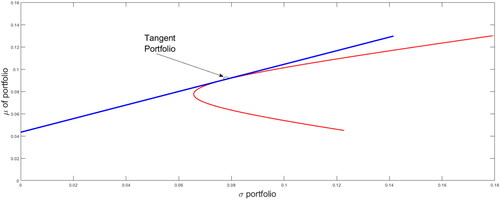
The set of points that contains this linear combination is called the capital market line. Investors choose one of these portfolios in the capital market line according to their degree of risk aversion. To determine the optimal weights of the tangent portfolio, it is necessary to consider expected returns ($\overrightarrow{\mu }$), the return of the risk-free asset (r_f), and the covariance matrix (Σ). The optimal weights ($w^{*}$) are obtained as $$w^{*}=\frac{{\Sigma }^{-1}(\overrightarrow{\mu }-r_f\overrightarrow{e_n})}{\gamma },$$ where γ is the reduction in an investor’s risk aversion. The practical application depends on obtaining good estimates of $\overrightarrow{\mu }$ and Σ. However, this approach is not simple in practice. In fact, Markowitz’s model has received serious criticism, including its poor out-of-sample performance (Bloomfield et al., 1977; DeMiguel et al., 2009; Kritzman et al., 2010) and the extreme weights of the resulting optimal portfolios (Black & Litterman, 1991, 1992; Papp et al., 2005). It has also been criticised because its optimal portfolio weights are highly sensitive to the dataset that is used to estimate the parameters, which generates high transaction costs (Best & Grauer, 1991; Chopra, 1993; Jobson & Korkie, 1981).

Several researchers have studied the impact of parameter estimation errors on portfolio optimisation. For instance, Chopra (1993) states that the major problems of the mean/variance (MV) framework are the errors associated with the estimation of the means, variances, and correlations of asset returns, as well as the fact that the optimisation process that underlies this methodology maximises these errors. In addition, Chopra and Ziemba (1993) indicate that the estimation errors in means are approximately 11 times more important than those in variances, and that the estimation errors in variances are about twice as important as those in covariances. Merton (1980) states that a long-term series of data is required to estimate expected returns accurately. Ng et al. (2020) explain the difficulty of improving the accuracy of estimates of the means of returns—even as the sample size increases. Moreover, Best and Grauer (1991) find that for an MV-efficient portfolio weight, both means and variances can be extremely sensitive to changes in asset means; consequently, they have implications for portfolio management. Researchers have also studied the effect of risk estimation on the performance of the Markowitz rule and the conditions required for good performance. For instance, Jobson and Korkie (1981), using Monte Carlo simulations, find that the mean, variance, and covariance parameters do not lend themselves to making inferences in small samples, even when considering 313 months or 26 years to calculate these parameters. Similarly, Jorion (1986) shows that, like local portfolios, the optimal asset allocation is sensitive to estimation risk in international cases. Michaud (1989) states that MV models are highly sensitive to changes in parameters and are hard to estimate; moreover, they also magnify the effect of estimation errors.

Researchers have consequently proposed amendments to the Markowitz model, which can be classified into four categories: the Bayesian approach (Barry, 1974; Black & Litterman, 1991, 1992; Brown, 1979; Jorion, 1986; Klein & Bawa, 1976), models with moment restrictions (MacKinlay & Pástor, 2000), models with a portfolio restriction (Best and Grauer, 1992), and the optimal combination of portfolios (Garlappi et al., 2007; Kan & Zhou, 2007).

The most popular approach to managing the effect of estimation risk is the use of Bayesian shrinkage estimators, which shrink the sample estimator towards a certain target under the premise that the resulting shrinkage estimator contains less estimation error than the sample estimator. For example, Jorion (1986) and Frost and Savarino (1986) use a shrinkage estimator of the means vector, Ledoit and Wolf (2003, 2004b, 2019, 2020) and Ollila and Raninen (2019) consider shrinking the covariance matrix, and DeMiguel et al. (2013) consider different combinations of the shrinkage of the means vector and covariance matrix. However, these proposed amendments have not eliminated the main practical drawbacks of the Markowitz model. Despite these amendments, out-of-sample performance is not superior to the naive $1/n$ rule and the weights of optimal portfolios obtained with these amendments remain extremely sensitive.

In this study, we contribute to the literature on this topic by proposing a new approach that largely overcomes all of these drawbacks. In addition to decreasing the effect of the estimation risk of the covariance matrix, we focus on reducing the negative effects of the presence of eigenvalues close to zero in the sample covariance matrix.

Our approach compresses the eigenvalue spectrum of a covariance matrix towards the eigenvalue spectrum of a diagonal matrix, which only contains the estimated values of the variances. This diagonal matrix target represents a multivariate process in which the variables are not correlated. Our approach is based on Ledoit and Wolf (2004b) and Schäfer and Strimmer (2005). In particular, the justification for our approach stems from random matrix theory (RMT). The application of RMT to portfolio optimisation suggests that the estimation risk of the correlation (or covariance) matrix plays an important role in this problem. Using these approaches, Laloux et al. (1999) establish that the smallest eigenvalues of this matrix are sensitive to estimation risk, whereas it is precisely those eigenvectors that correspond to the smallest eigenvalues that determine (in Markowitz’s theory) the least risky portfolios.

To take advantage of this approach, we must determine the optimal shrinkage degree of the covariance matrix before choosing the optimal portfolio. Therefore, we propose a method that makes the smallest eigenvalue of the fitted correlation matrix larger than the minimum corresponding to a random matrix. Next, we compare the performance of our proposed method with the Markowitz method without adjustments, the $1/n$ rule, the Ledoit and Wolf (2003, 2004a, b, 2020) methods, and the two methods proposed by Ollila and Raninen (2019). We find that the proposed method delivers better out-of-sample performance than all of the other methods for sample sizes larger than 165 months and maintains more stable and less volatile financial asset weights. Our results show that the proposed approach permits the Markowitz rule to clearly overcome the $1/n$ rule, which shows a notable decrease in the extreme values of the optimal portfolio weights and at the same time a significant decrease in the volatility of the optimal portfolio weights. Moreover, these results are obtained when using relatively small sample sizes to estimate the parameters.

The traditional corrections to the MV model have typically centred on raising its performance by improving the estimations of the parameters and diminishing the risk of the estimation. However, in most of these corrections, the weights of the resulting portfolios continue to be highly volatile. Unfortunately, this makes the practical application of the unrestricted model unviable because of the high transaction costs implied by the extreme changes in the portfolio weights. For example, using the methodologies of Ledoit and Wolf (2003, 2004a, b, 2020) and Ollila and Raninen (2019), we show that it is possible to improve the performance of the MV model but that the high volatility of the optimal weights prevails. The sensitivity of the optimal weights is only strongly attenuated when near-zero eigenvalues of the covariance matrix are shifted into the space that those of a random matrix occupy.

The following sections are organised as follows. Section 2 presents the eigenvalue shrinkage model. Section 3 describes the procedures that we followed to perform the out-of-sample comparisons of the portfolio selection rules. Section 4 shows the preliminary results, while highlighting the potential advantages. Section 5 presents the advantages of applying a new portfolio selection rule and compares the out-of-sample performance with other covariance matrix shrinkage proposals. Finally, Section 6 concludes.

2. The model

In this section, we will develop a covariance matrix estimate based on the shrinkage of the eigenvalue spectrum.

2.1. Traditional Markowitz approach

Consider that we have a set of T observations of n financial assets with returns r_it for $i=1,2,3\dots ,n,$ with $t=1,2,3,\dots T,$ and a risk-free asset that investors can lend and borrow without limit up to the rate r_f.

We assume that investors who wish to determine their optimal portfolios use a fixed sample size of the latest m observations to estimate the parameter values: the risk premiums of each asset (the average return less the return of a risk-free asset) ${\mu }_i-r_f$ and the covariance matrix Σ.

Typically, in the portfolio selection model, it is assumed that investors have utility functions of the following type: $$U({\mu }_p,{\sigma }_p)={\mu }_p-\frac{1}{\gamma }{\sigma }_p^2\mathrm{\hspace{1em}}\mathrm{\hspace{1em}}(1)$$ where μ_p is the expected return of the portfolio chosen by the investor, σ_p is the respective variance of the portfolio, and γ represents the risk aversion of the investor. This theory assumes that investors seek to maximise their utility function, with the restriction that the invested money is divided among a set of financial assets that contains n risky assets and one risk-free asset. Hence, ${\mu }_p={\mathit{w}}^{\mathit{t}}\mathit{\mu }+(1-{\mathit{w}}^{\mathit{t}}\mathit{e})r_f,$ and ${\sigma }_p^2={\mathit{w}}^{\mathit{t}}\Sigma \mathit{w},$ where ${\mathit{w}}^{\mathit{t}}=[w_1,w_2,w_3\dots w_n]$ is the weight assigned to each risky asset and e is the column vector of ones of dimension n. Therefore, the problem for the investor is (1) $$ma{x}_{\mathit{w}}[{\mathit{w}}^t\mathit{\mu }+(1-{\mathit{w}}^t\mathit{e})r_f-\frac{\gamma }{2}{\mathit{w}}^t\Sigma \mathit{w}]$$(1)

The solution is (2) $${\mathit{w}}^{*}=\frac{{\Sigma }^{-1}(\mathit{\mu }-\mathit{e}{r}_f)}{\gamma }$$(2)

Investors can invest money in a risk-free asset that has a return of r_f, and in n risky assets that have expected returns $\mathit{\mu }$ and a covariance matrix Σ. They can assign a percentage of their wealth to each risky asset ${\mathit{w}}^t=[w_1,w_2,w_3,\dots w_n]$ and $(1-{\mathit{w}}^t\mathit{e})$ to the risk-free asset.² Following this reasoning, Tobin (1958) demonstrates that investors can achieve optimal portfolios by investing a proportion of their wealth in the risk-free asset and the remainder in a portfolio that contains only risky assets ${\mathit{w}}_{\mathit{T}},$ which can be determined as (3) $${\mathit{w}}_{\mathit{T}}=\frac{{\Sigma }^{-1}(\mathit{\mu }-\mathit{e}{r}_f)}{{\mathit{e}}^t{\Sigma }^{-1}(\mathit{\mu }-\mathit{e}{r}_f)}$$(3)

Therefore, using this approach to determine how investors have to invest entails inverting the covariance matrix Σ and multiplying it by the expected excess returns of the risky assets over the risk-free asset $\mathit{\mu }-\mathit{e}{r}_f.$ However, it is difficult in practice to estimate the true value of these parameters given that they are mainly obtained using limited historical data. Thus, the estimation risk of these parameters sharply affects the performance of the optimal rule of investment proposed by Markowitz (1952).

If investors consider m preview observations of n assets $r_{it}i=1,2,\dots ,nt=1,2,\dots ,m,$ then the means and covariances are estimated using the following expressions: (4) $${\widehat{\mu }}_i=\frac{\sum _{i=1}^m{r}_{it}}{m}$$(4) and (5) $${\widehat{\Sigma }}_{ij}=\frac{\sum _{i=1}^m(r_{it}-{\widehat{\mu }}_i)(r_{jt}-{\widehat{\mu }}_j)}{m-1}$$(5)

Consequently, the empirical optimal portfolio weights are determined by (6) $${\widehat{\mathit{w}}}_{\mathit{T}}=\frac{{\widehat{\Sigma }}^{-1}(\widehat{\mathit{\mu }}-\mathit{e}{r}_f)}{{\mathit{e}}^t{\widehat{\Sigma }}^{-1}(\widehat{\mathit{\mu }}-\mathit{e}{r}_f)}$$(6)

2.2. Shrinkage estimation of the eigenvalues of the covariance matrix

In this study, we propose a new approach that compresses the eigenvalue spectrum of a covariance matrix towards the eigenvalue spectrum of a diagonal matrix, which only contains the estimated values of the variances to move the eigenvalues of the covariance matrix away from zero. This diagonal matrix target represents a multivariate process in which the variables are not correlated among themselves. This approach is similar to the approach that was proposed by Ledoit and Wolf (2004b) and Schäfer and Strimmer (2005).

The justification for our approach stems from RMT. The application of RMT to portfolio optimisation suggests that the estimation risk of the correlation (or covariance) matrix plays an important role in this problem. Using this approach, Laloux et al. (1999) find that the smallest eigenvalues of this matrix are sensitive to estimation risk, whereas it is precisely the eigenvectors corresponding to the smallest eigenvalues that determine (in Markowitz’s theory) the least risky portfolios. Thus, as stated by Laloux et al. (1999), ‘one should be careful when using this correlation matrix in applications.’

RMT establishes that for a dataset X that has T observations of n random variables with dimension n × T, where all its components are independent random variables, the spectrum of eigenvalues of its covariance matrix [$C=\frac{X^{t}X}{T}-\overrightarrow{\mu }{\overrightarrow{\mu }}^t$] will be between a minimum limit ‘$a$’ and a maximum limit ‘$b$’ (see Marchenko & Pastur, 1967), where (7) $$a={\sigma }^2{(1-\sqrt{\frac{n}{T}})}^2,b={\sigma }^2{(1+\sqrt{\frac{n}{T}})}^2$$(7)

As we will show later, the eigenvalues below the lower limit ‘$a$’ contain problematic noise that complicates the portfolio optimisation process. Furthermore, smaller eigenvalues determine (in Markowitz’s theory) the least risky portfolios. Eigenvalues between ‘$a$’ and ‘$b$’ are noise belonging to random matrix-type behaviour, whereas values greater than ‘$b$’ contain useful information. In this study, we propose an adjustment of the covariance matrix by shrinking the covariance matrix eigenvalue spectrum towards a target eigenvalue spectrum. The matrix associated with this target is a diagonal matrix containing the values of the estimated variances on its diagonal. This target matrix mimics a random matrix because the covariances between the variables considered are zero.

This methodology aims to move the part of the eigenvalue spectrum of the covariance matrix that lies between zero and ‘a’ within the eigenvalue spectrum sector given by RMT; that is, the region (a, b). The benefit of applying this adjustment to the covariance matrix is the noticeable reduction in the dispersion of the optimal portfolio weights without any restrictions on them, which allows us to obtain stable portfolios that imply low transaction costs for investors and a considerable improvement in the performance of the Markowitz rule. In fact, the out-of-sample Sharpe ratio surpasses the $1/n$ rule, which permits investors to obtain higher returns for each risk level.

We propose the following correction of the covariance matrix to calculate the optimal weights: (8) $$\widehat{Y}=(1-\eta )\widehat{\Sigma }+\eta \widehat{S}$$(8) where $\widehat{S}$ is the diagonal matrix of $\widehat{\Sigma }$ and η is an adjustment factor of the shrinkage. This is the same expression that Schäfer and Strimmer (2005) employ when two models are used to estimate the covariance matrix, the first with many free parameters and the second with little bias.

Consequently, the optimal weights are (9) $${\mathit{w}}_{\mathit{MaC}}=\frac{{\widehat{Y}}^{-1}(\widehat{\mathit{\mu }}-\mathit{e}{r}_f)}{{\mathit{e}}^t{\widehat{Y}}^{-1}(\widehat{\mathit{\mu }}-\mathit{e}{r}_f)}$$(9)

2.2.1. Shrinkage of the eigenvalue spectrum

Each of the n eigenvalues of the covariance matrix $\widehat{\Sigma },$ ${\lambda }_{\Sigma },$ can be estimated by (10) $$\det ({\lambda }_{\Sigma (i)}I-\widehat{\Sigma })=0$$(10)

Furthermore, each of the n eigenvalues of the matrix $\widehat{Y},$ λ_Y, can be obtained by (11) $$\det ({\lambda }_{Y(i)}I-(1-\eta )\widehat{\Sigma }-\eta \widehat{S})=0$$(11)

The eigenvalues of the matrix $\widehat{Y},$ λ_Y, are those of the matrix Ω when η = 0; as η increases, they approach those of the diagonal matrix S and for η = 1 they are equal to those of the S matrix. Consequently, by changing η, we shift the eigenvalues of the matrix $\widehat{Y}.$

2.2.2. Eigenvalue spectrum of a typical large covariance matrix

The random matrix eigenvalues have the following distribution³: (12) $$\lambda =\{\begin{array}{cc}\frac{1}{2\pi xy{\sigma }^2}\sqrt{(b-x)(x-a)}\hfill & a<x<b\hfill \\ 0\hfill & \text{otherwise}\hfill \end{array}$$(12) where a and b are given by Eq. (7)(7) $$a={\sigma }^2{(1-\sqrt{\frac{n}{T}})}^2,b={\sigma }^2{(1+\sqrt{\frac{n}{T}})}^2$$(7) and $y=\frac{n}{T}.$

The red line in Figure 2 shows the theoretical density of the eigenvalues of the random correlation matrix with dimensions equal to 30. The empirical density function of the eigenvalues is shown by the blue line of the correlation matrix of the 30 equally weighted industrial portfolios⁴ considering a sample size of 200 monthly observations⁵ In total, the eigenvalues of the 938 correlation matrices are used to construct this density function.

Figure 2. Density of the eigenvalues of the covariance matrix Σ and of a random matrix.

Source: Authors.

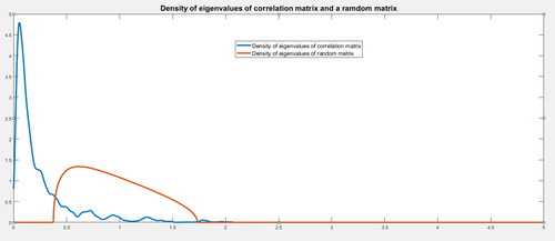
A high proportion of the eigenvalues are below the lower limit of an associated random matrix. As we will show later, the presence of these eigenvalues in this area causes serious problems for the Markowitz model.

Although not shown in Figure 2, the empirical function of the density of the eigenvalues of Σ reaches values up to 25. According to these observed values and principal component theory, this means that the highest eigenvalue explains around 83% of the variance, while smaller eigenvalues explain a minimal part of the variance of the covariance matrix.

According to RMT, the presence of eigenvalues below the lower limit (a = 0.3754 for n = 30) is highly problematic when determining the optimal portfolio according to Markowitz (Bai et al., 2009). By contrast, eigenvalues above the upper limit b = 1.7325 contain valuable information, while eigenvalues within these limits $[a,b]$ are the products of a random matrix. The proposed approach allows us to move the spectrum of eigenvalues towards a space in which all of these values are above the lower limit of the spectrum corresponding to a random matrix.

2.2.3. Another explanation of the optimal weight sensitivity from the spectral decomposition

A square symmetric matrix such as a covariance matrix can be expressed as (13) $$\Sigma =UD{U}^{-1}$$(13) where U is defined as (14) $$U=[{\mathit{u}}_1,{\mathit{u}}_2,{\mathit{u}}_3,\dots {\mathit{u}}_n]$$(14)

Here, ${\mathit{u}}_i$ represent the eigenvectors of the matrix Σ and D is a diagonal matrix containing the eigenvalues ${\lambda }_{\Sigma }$ of the matrix Σ. Therefore, we can express (15) $$\Sigma =\sum _{i=1}^n{\lambda }_i{\mathit{u}}_{\mathit{i}}{\mathit{u}}_{\mathit{i}}^{\mathit{t}}$$(15) where $u_i{u}_i^t$ are matrices with a rank equal to one. In a similar way, we can express the inverse of a covariance matrix as (16) $${\Sigma }^{-1}=\sum _{i=1}^n{\lambda }_i^{-1}{\mathit{u}}_{\mathit{i}}{\mathit{u}}_{\mathit{i}}^{\mathit{t}}$$(16)

Eq. (16)(16) $${\Sigma }^{-1}=\sum _{i=1}^n{\lambda }_i^{-1}{\mathit{u}}_{\mathit{i}}{\mathit{u}}_{\mathit{i}}^{\mathit{t}}$$(16) shows that when we invert a matrix, smaller eigenvalues and their corresponding eigenvectors are more important than larger eigenvalues. Furthermore, the estimation error of the smallest eigenvalue is greater than that of the highest eigenvalue. This shows the sensitivity of the Markowitz model to errors in the assessment of smaller eigenvalues. Figure 2 shows the eigenvectors associated with eigenvalues with a mean of 0.06, which determine the inverse matrix of Eq. (16)(16) $${\Sigma }^{-1}=\sum _{i=1}^n{\lambda }_i^{-1}{\mathit{u}}_{\mathit{i}}{\mathit{u}}_{\mathit{i}}^{\mathit{t}}$$(16) . The eigenvector associated with the highest eigenvalue, whose value is equal to 25, has minimal importance.

Traditional methodologies aim to reduce the effects of risk in the estimation of the parameters. However, if, after these corrections, the covariance matrix that is finally used continues to have values close to zero, then the high sensitivity of the optimal weights will continue. Thus, for the MV method to be viable, it must try to diminish the estimation risk of the parameters and shift the values of the covariance matrix itself towards the centre in which those of a random matrix are located.

3. Data and experiment

The data correspond to the 1138 monthly observations of excess returns on the risk-free asset of 30 industrial portfolios from July 1926 to April 2021. These are the 30 equally weighted industrial portfolio sectors taken from Kenneth French’s website. We use the series of one-month Treasury bills taken from the Federal Reserve Economic Data as the risk-free rate.

To compare the relative empirical performance of the Markowitz rule with the shrinkage of eigenvalues, we use the naive $1/n$ rule as a benchmark. This investment rule invests a proportion of $1/n$ of wealth in each of the n assets available for investing in each of the rebalancing dates. We use this naive rule as the benchmark because it is easy to implement given that no parameter estimation is necessary. Hence, this rule has not been outperformed by more complex optimisation rules when small sample sizes are used to estimate the parameters.⁶ Furthermore, this rule does not involve any parameter estimation or optimisation process and the data do not matter: (17) $$w_{1/n}=\frac{1}{n}$$(17)

We use a rolling sample approach that is similar to the one that was used by DeMiguel et al. (2009). Given a dataset of T = 1138 monthly observations, we use sample sizes ($m$) that are equal to 200, 300, 400, and 500 monthly observations. For the case in which the investor uses a sample size of m, we thus have $(T-m)$ observations of realised returns obtained using the investment rule suggested by each model.

The observations of out-of-sample returns are used to analyse the performance of these investment rules. The assumptions of the empirical models are as follows:

1. Investors use the first m observations to estimate the parameter values (mean and covariance matrix).

2. Using these parameters, investors compute the optimal portfolio weights.

3. Then, they use this asset allocation to build their portfolios.

4. Investors hold their investments in these portfolios for one month.

5. At the end of the month, they calculate their realised returns.

6. At the beginning of the following month, investors choose the last $m$ months to recalculate the parameters by dropping the earliest return and adding the return of the following month. In this way, the number of monthly observations that is used to calculate the parameters is always equal to m.

7. Steps from 2 to 6 are repeated until investors take the last assignation in month $T-m.$

As explained earlier, for each sample size of length m, we have $(T-m)$ observations of realised excess returns, which are calculated as follows: (18) $${\pi }_{\mathit{realized}}(k)={\mathit{\pi }}_{m+k}^t{\widehat{\mathit{w}}}_{\mathit{rule}}k=1,2,\dots ,(T-m),$$(18) where the value of ${\widehat{\mathit{w}}}_{\mathit{rule}}$ depends on the investment rule used:

1. If we use the Markowitz rule, ${\widehat{\mathit{w}}}_{\mathit{rule}}={\widehat{\mathit{w}}}_{\mathit{opt}}.$

2. If we use the Markowitz rule with the proposed adjustment, ${\widehat{\mathit{w}}}_{\mathit{rule}}={\widehat{\mathit{w}}}_{\mathit{optR}}.$

3. If we use the $1/n$ rule, ${\widehat{w}}_{\mathit{rule}}(i)=1/n$ for $i=1,2,..,n.$

Thus, we have $(T-m)$ observations of realised excess returns for the three rules. Using these realised excess returns, we calculate the out-of-sample Sharpe ratio for the three rules: (19) $${\pi }_{\mathit{average}}=\frac{\sum _{i=1}^{T-m}{\pi }_{\mathit{realized}}(m+i)}{(T-m)}$$(19) (20) $${\sigma }_{\mathit{average}}=\sqrt{\frac{\sum _{i=1}^{T-m}{({\pi }_{\mathit{realized}}(m+i)-{\pi }_{\mathit{average}})}^2}{(T-m-1)}}$$(20)

Then, we calculate the realised Sharpe ratio (21) $$SR(m)=\frac{{\pi }_{\mathit{average}}}{{\sigma }_{\mathit{average}}}$$(21)

For m = 200, we have 938 observations to compute the out-of-sample Sharpe ratio; for the other extreme (m = 500), we have 638 observations. This allows us to assess the performance of the three investment rules for sample sizes of 200, 300, 400, and 500 months.

Recall that we assume that investors choose their portfolios at the beginning of each month and then rebalance their portfolios by considering the results obtained and the new optimal weightings chosen at the end of the month. It would thus be interesting to explore the optimal length of portfolio rebalancing (e.g. Fahmy, 2020).

4. Preliminary results of the shrinkage estimations

4.1. Results using the 30 equally weighted industrial portfolios

Figure 3 shows the results obtained using a rolling sample size of 200 monthly observations.

Figure 3. Out-of-sample Sharpe ratio for different shrinkage levels for a sample size of 200.

Source: Authors.

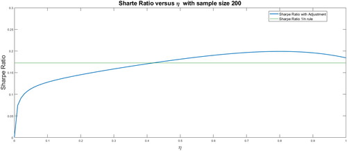
Figure 3 shows the out-of-sample Sharpe ratio for the different investment rules. The green line shows the Sharpe ratio of the naive rule $1/n$ and the blue line shows the out-of-sample modified Markowitz Sharpe ratio for values of η ranging from 0 to 1, with an increment of 0.01. The Markowitz rule without shrinkage corresponds to η equal to zero. The Sharpe ratio of the Markowitz rule without restriction, for a sample size of 200, is 0.011. This is well below that obtained using the $1/n$ rule, which has an out-of-sample Sharpe ratio of 0.1725. The out-of-sample Sharpe ratio rises by increasing the value of η until it peaks at 0.1990. This optimal adjustment is obtained for η equal to 0.81. Moreover, with the optimum shrinkage, the out-of-sample Sharpe ratio increases from 0.03 to 0.1990 (i.e. an 18-fold increase).

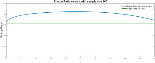
Figure 4 shows the out-of-sample Sharpe ratio for a sample size of 300. The Sharpe ratio without adjustment is 0.1641, which is higher than that obtained using the $1/n$ rule (0.1581). In this case, the optimal adjustment is obtained for η equal to 0.47 with a Sharpe ratio of 0.2117; that is, the out-of-sample Sharpe ratio increases by 29% with respect to the Markowitz rule without adjustment.

Figure 4. Out-of-sample Sharpe ratio for different shrinkage levels for a sample size of 300.

Source: Authors.

Figure 5 shows that the Sharpe ratio without adjustment is 0.1480, which is higher than that obtained using the $1/n$ rule (0.1424). In this case, the optimal adjustment is obtained for η equal to 0.43, with a Sharpe ratio of 0.1945; that is, the out-of-sample Sharpe ratio increases by 31% with respect to the Markowitz rule without adjustment.

Figure 5. Out-of-sample Sharpe ratio for different shrinkage levels for a sample size of 400.

Source: Authors.

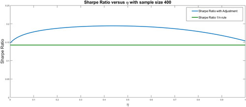
Figure 6 shows that the Sharpe ratio without adjustment is 0.1412, which is higher than that obtained using the $1/n$ rule of 0.1305. In this case, the optimal adjustment is obtained for η equal to 0.37, with a Sharpe ratio of 0.1889; that is, the out-of-sample Sharpe ratio increases by 34% with respect to the Markowitz rule without adjustment.

Figure 6. Out-of-sample Sharpe ratio for different shrinkage levels for a sample size of 500.

Source: Authors.

In summary, the compression of the covariance matrix to a random matrix improves the out-of-sample Sharpe ratio for all of the sample sizes that we considered. However, its effect is stronger for smaller sample sizes.

4.2. Effects of the optimal weights

Recalling that the low performance of the Markowitz rule is only one of its drawbacks, we now focus on the second drawback (i.e. its extreme and volatile portfolio weights).

To illustrate this issue, the following exercise is carried out:

• We calculate the 30 portfolio weights obtained with the Markowitz rule without adjustment for each of the $(T-m)$ portfolios.

• We calculate the 30 portfolio weights obtained with the Markowitz rule with the optimal adjustment for each of the $(T-m)$ portfolios.

• We calculate the means and standard deviations of each portfolio weight.

Table 1 shows the means and standard deviations of the optimal weights of the Markowitz rule with and without the adjustment for each of the 30 equally weighted industrial portfolios. Columns 2 and 4 show the means of the optimal weights obtained with the Markowitz rule without adjustment for sample sizes of 200 and 500 monthly observations, and columns 3 and 5 show their respective standard deviations. Similarly, columns 6 and 8 show the means of the optimal weights obtained using the Markowitz rule when setting the optimum adjustment to the covariance matrix for sample sizes of 200 and 500 monthly observations, and columns 7 and 9 show their respective standard deviations.

Table 1. Means and standard deviations of the portfolio weights.

Values of weights
Markowitz rule without adjustment					Markowitz rule with optimal Adjustment
	Sample size 200		Sample size 500		Sample size 200		Sample size 500
	Mean	Standard deviation	Mean	Standard deviation	Mean	Standard deviation	Mean	Standard deviation
1	0.61	4.11	0.29	0.19	0.08	0.06	0.13	0.05
2	−0.58	5.88	−0.15	0.21	0.04	0.16	0.00	0.11
3	0.38	3.72	0.25	0.09	0.10	0.10	0.20	0.04
4	−0.04	1.14	−0.21	0.28	−0.01	0.05	−0.07	0.06
5	0.27	2.87	0.21	0.40	0.03	0.09	0.07	0.11
6	−0.63	1.92	−0.54	0.27	0.00	0.03	−0.07	0.03
7	−0.18	1.89	−0.16	0.26	0.00	0.05	−0.08	0.05
8	−0.24	2.77	0.29	0.17	0.06	0.08	0.15	0.06
9	0.31	1.56	0.24	0.34	0.04	0.06	0.08	0.06
10	−0.21	3.90	−0.16	0.16	−0.01	0.07	−0.10	0.05
11	0.41	5.59	−0.21	0.16	0.01	0.02	−0.04	0.02
12	−1.11	5.06	−0.38	0.21	0.00	0.04	−0.07	0.03
13	0.12	1.30	0.16	0.24	0.02	0.03	0.01	0.03
14	0.44	8.09	−0.09	0.24	0.02	0.05	−0.02	0.04
15	−0.31	3.27	−0.02	0.23	0.00	0.04	−0.05	0.04
16	0.27	1.59	0.26	0.15	0.04	0.06	0.07	0.05
17	0.36	0.88	0.16	0.13	0.03	0.09	0.06	0.05
18	0.15	0.81	0.04	0.12	0.03	0.11	0.03	0.06
19	0.53	3.18	0.12	0.23	0.06	0.12	0.11	0.11
20	−0.19	6.34	0.20	0.17	0.15	0.21	0.28	0.17
21	0.63	7.28	0.31	0.21	0.05	0.09	0.14	0.08
22	0.35	1.03	0.23	0.16	0.04	0.05	0.09	0.06
23	−0.13	3.61	−0.06	0.26	0.03	0.05	0.01	0.04
24	0.37	2.08	0.29	0.26	0.03	0.07	0.07	0.05
25	−0.32	2.59	−0.23	0.10	0.01	0.04	−0.05	0.02
26	−0.29	2.65	−0.16	0.24	0.02	0.06	−0.03	0.05
27	0.20	1.15	0.07	0.18	0.03	0.04	0.02	0.03
28	−0.12	0.74	−0.11	0.15	0.00	0.06	−0.06	0.07
29	0.20	2.03	0.39	0.45	0.07	0.14	0.12	0.11
30	−0.24	4.43	−0.01	0.17	0.03	0.04	0.00	0.03

Source: Authors.

The observed means and standard deviations of the optimal weights obtained using the traditional Markowitz rule show that the weights are extremely high and volatile. For example, for a sample size of 200, the mean of the number 11 portfolio weight of the industrial portfolio is −1.11. Therefore, investors who want to use this rule would have to invest taking the short position in this asset by 1.11 times their wealth. Additionally, the standard deviation of this asset is 5.59 times the value of investors’ wealth, which implies high transaction costs for investors. These facts make it infeasible to use the Markowitz rule under these conditions.

Certainly, these values are the most extreme when the sample size is small. However, the number of observations considered in the sample size does not eliminate these drawbacks. This is consistent with the findings of Jobson and Korkie (1981), Chopra and Ziemba (1993); Chopra (1993), and Best and Grauer (1991)

Instead, using the Markowitz rule with the optimum shrinkage of the eigenvalue spectrum of the covariance matrix, we obtain smaller values with a lower dispersion for each asset weight. For a sample size of 200 monthly observations, the dispersion of some of the weights decreases by more than 416 times.

In conclusion, using this approach improves the out-of-sample Sharpe ratio and at the same time lowers the volatility of the portfolio weights markedly. This could allow the Markowitz rule to overcome its main practical drawbacks.

4.3. Effects of the eigenvalues of the covariance matrix

To assess whether the eigenvalue spectrum is affected using this approach, we calculate the eigenvalues λ_i for all of the samples and determine the percentage of times that they are within the limits associated with a random matrix. For a sample size of 200 monthly observations, we calculate the 30 eigenvalues of the 938 correlation matrices with and without shrinkage. Table 2 shows the results, where the values presented are averages. This shows that the main effect of the adjustment is to reduce the percentage of times that the eigenvalues are below the minimum limit.

Table 2. The effect of the eigenvalues of the covariance matrix.

Percentage of times
	Sample size 200		Sample size 500
	Without adjust	With optimal adjust	Without Adjust	With optimal Adjust
Eigenvalues less than inferior limit	77.47%	0.00%	88.00%	0.00%
Eigenvalues higher than superior limit	3.56%	3.33%	3.33%	3.33%

Source: Authors.

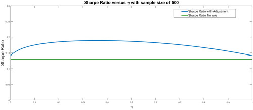
The abundant noise in the estimation of the covariance matrix values triggers the greater presence of eigenvalues below the lower limit, as established in the spectral density of Marchenko and Pastur (1967). Larger eigenvalues remain relatively unaffected by the effect of noise.⁷ Figure 7 shows that the eigenvalues spectrum moves towards the right as the compression of the covariance matrix to a random matrix increases. Initially, a large proportion of eigenvalues are below the lower random matrix limit. Meanwhile, as we reach the optimal shrinkage level, no eigenvalues are below the lower limit.

Figure 7. Density of the eigenvalues for different degrees of compression.

Source: Authors.

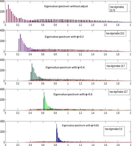
Figure 7 shows the effect of the shrinkage degree (by increasing η) over the eigenvalue spectrum. Random matrix density is shown in brown for all the figures. As the value of η increases, the eigenvalue spectrum of the shrinking matrix shifts towards the interior of a random matrix spectrum. For $\eta =0.81,$ the lowest eigenvalues of the compressed matrix are all inside the random matrix spectrum.

5. Estimating the optimal covariance matrix ex-ante shrinkage level

So far, we have shown that the shrinkage of the covariance matrix can significantly improve the performance of the Markowitz rule. However, we now want to explore how effective this method is under more realistic conditions. In practice, an investor must simultaneously determine both the degree of compression of the covariance matrix and the portfolio in which they will invest, using only the information available up to that point. Thus, the investor must determine the ex-ante shrinkage level. A comparison with other approaches used to shrink the covariance matrix is also required. For example, we compare our method with the one proposed in Ledoit and Wolf (2004b), followed by a comparison of the optimal shrinkage with other more recent approaches.

5.1. Ledoit–Wolf approach

The Ledoit and Wolf (2004b) method minimises the estimation risk of a set of parameters by shrinking them to a target set value. The logic of this approach relies on the fact that the covariance matrix has a high estimation risk due to the presence of many degrees of freedom. Therefore, this shrinkage to another biased one (with a lower estimation risk and fewer degrees of freedom) reduces the effects of the estimation risk.

Using Ledoit and Wolf (2004b), we estimate the optimal shrinkage for the 938 samples of size 200.

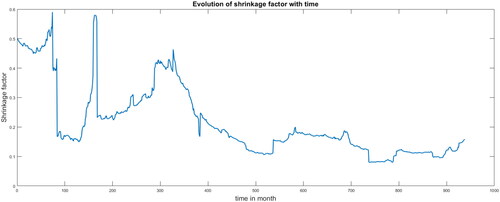
Figure 8 shows the optimal shrinkage values for each one of the 938 considered samples (of size 200 observations). It shows that the shrinkage degree value decreases when the samples use more recent data. Using these values, we calculate the Markowitz out-of-sample Sharpe ratio and obtain a value of 0.0835 compared with 0.1564 for the $1/n$ rule. This result shows that although the estimation risk decreases, it is not sufficient to ensure that the Markowitz rule performs better than the $1/n$ rule.

Figure 8. Shrinkage for a sample size of 200 months.

Source: Authors.

5.2. Shrinkage of the eigenvalues of the covariance matrix

Considering this discussion and recalling that the eigenvalues of the covariance matrix below the lower limit of the eigenvalues of a random matrix are those that cause greater problems to the Markowitz rule, we propose an alternative shrinkage approach. This approach consists of moving the smaller eigenvalues within the limits of the respective random matrix. Specifically, we calculate the eigenvalues λ_i of the correlation matrix. We then take the minimal eigenvalue λ_min and move it towards the random matrix spectrum: (22) $$\eta \times {\lambda }_{\mathit{min}}+(1-\eta )\times 1\ge {(1-\sqrt{\frac{n}{T}})}^2$$(22)

From equation 22(22) $$\eta \times {\lambda }_{\mathit{min}}+(1-\eta )\times 1\ge {(1-\sqrt{\frac{n}{T}})}^2$$(22) , we choose the shrinkage factor ${\eta }^{*}$ as (23) $${\eta }^{*}=\frac{1-{(1-\sqrt{\frac{n}{T}})}^2}{1-{\lambda }_{\mathit{min}}}$$(23)

Henceforth, we call this approach the optimal shrinkage of the covariance matrix eigenvalues (OSME). We calculate the optimal ${\eta }^{*}$ for 938 samples and show the result in Figure 9. Thus, for each of the 938 samples with 200 monthly observations, a new correlation matrix is determined using $$\widehat{Y}=(1-{\eta }^{*})\widehat{\Sigma }+{\eta }^{*}\widehat{S}$$

Figure 9. Shrinkage for a sample size of 200 months.

Source: Authors.

Figure 9 shows that the shrinkage levels have higher and more stable values than the Ledoit and Wolf (2004b) approach. Next, we calculate the out-of-sample performance of the Markowitz rule using this approach. We find that its Sharpe ratio is equal to 0.1928, which is slightly above that of the $1/n$ rule (0.1564).

5.3. Comparison between OSME, Ledoit–Wolf, and the $1/n$ rule

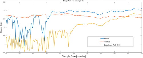
In this subsection, we first compare OSME Ledoit and Wolf (2004a) with the $1/n$ rule. Figure 10 shows the Sharpe ratio of the $1/n$ rule in red, that obtained using the Ledoit–Wolf method in brown, and that obtained using OSME in blue for the different sample sizes. This figure shows that the $1/n$ rule is higher for sample sizes of less than 165 months. OSME performs better for sample sizes greater than 165 months. The Ledoit–Wolf method begins to be higher than the $1/n$ rule for sample sizes over 280 months. However, it is never superior to OSME.

Figure 10. Out of-sample Sharpe ratio versus sample size.

Source: Authors.

Table 3 shows the means and standard deviations of the optimal weights obtained using these three approaches. Although the standard deviation of the weights decreases, it remains high. The volatility of the optimal weights under the OSME approach is the lowest. The results show notably better performance for the Markowitz rule with OSME adjusted with respect to the naive $1/n$ rule, and not only for a sample size of 200 months. This third approach allows the Markowitz rule to perform better than the $1/n$ rule for sample sizes greater than 165 monthly observations.

Table 3. Means and standard deviations of the portfolio weights.

Weight values
	Markowitz		Ledoit and Wolf (2004a,b)		OSME
	Mean	Standard deviation	Mean	Standard deviation	Mean	Standard deviation
1	0.61	4.11	0.13	0.19	0.08	0.04
2	−0.58	5.88	−0.14	0.43	0.04	0.09
3	0.38	3.72	0.22	0.30	0.10	0.06
4	−0.04	1.14	−0.12	0.16	−0.01	0.03
5	0.27	2.87	0.10	0.25	0.03	0.06
6	−0.64	1.92	−0.14	0.14	0.00	0.02
7	−0.18	1.89	−0.07	0.14	0.00	0.03
8	−0.25	2.77	0.18	0.19	0.06	0.04
9	0.31	1.56	0.08	0.20	0.04	0.03
10	−0.21	3.90	−0.14	0.20	−0.01	0.04
11	0.41	5.59	−0.05	0.11	0.01	0.01
12	−1.11	5.06	−0.16	0.17	0.00	0.02
13	0.12	1.30	0.01	0.10	0.02	0.02
14	0.44	8.09	−0.04	0.20	0.02	0.03
15	−0.32	3.27	−0.05	0.14	0.00	0.03
16	0.28	1.59	0.11	0.17	0.04	0.04
17	0.36	0.88	0.10	0.22	0.03	0.06
18	0.15	0.81	0.08	0.22	0.03	0.07
19	0.53	3.18	0.17	0.29	0.06	0.07
20	−0.19	6.34	0.21	0.46	0.15	0.14
21	0.63	7.28	0.22	0.26	0.05	0.05
22	0.35	1.03	0.10	0.11	0.04	0.03
23	−0.13	3.61	0.04	0.16	0.03	0.03
24	0.37	2.08	0.03	0.21	0.03	0.04
25	−0.32	2.59	−0.08	0.17	0.01	0.02
26	−0.29	2.65	−0.06	0.19	0.02	0.03
27	0.20	1.15	0.04	0.10	0.03	0.02
28	−0.12	0.74	−0.08	0.15	0.00	0.04
29	0.20	2.03	0.23	0.51	0.07	0.09
30	−0.24	443	0.0^4	0.10	0.03	0.03

Source: Authors.

5.4. Comparison with other approaches

Finally, to demonstrate the robustness of our results, we compare the proposed approach with recent approaches related to the shrinkage of covariance matrices. The methods that we consider are those of Ledoit and Wolf (2003, 2004a,b, 2020) and Ollila and Raninen (2019). All of these methods seek to decrease the estimation error in the covariance matrix by compressing the traditional matrix into an identity matrix to decrease the mean squared error. Table 4 shows the out-of-sample performance of several methods. Two methods developed by Ollila and Raninen (2019) are considered (Ell1-RSCM and Ell2-RSCM). The table shows that the $1/n$ rule predominates for sample sizes less than 200 months. Meanwhile, the OSME approach predominates for sample sizes of 150 months and over. The Ledoit–Wolf and Ollila–Raninen methods exceed the $1/n$ rule for a sample size greater than 300 months. The Sortino ratio is used as a performance measure to check the robustness of the results (Sortino & Van Der Meer, 1991). Whereas the Sharpe ratio considers the standard deviation σ as the risk measure, the Sortino ratio considers as risk only the part of σ whose values are below a minimum acceptable return. Table 5 shows the performance measures using the Sharpe and Sortino ratios for a sample size of 200 monthly observations. As before, the results continue to show the superior performance of the OSME method. We use the one-month Treasury bills as the minimum acceptable return to calculate the Sortino ratio.

Table 4. Out-of-sample performance.

Out-of-sample performance (Sharpe Ratio)
Sample Size	Markowitz	Rule 1/n	LW 2020	LW 2003	LW 2004 A	LW 2004 B	011ila 1	011ila 2	OSME
100	−0.0182	0.1692	−0.0249	−0.0278	0.0333	0.0395	0.0433	0.0152	0.1070
150	0.0356	0.1691	−0.0198	−0.0078	−0.0125	−0.0274	0.0320	0.0038	0.1125
200	0.0011	0.1725	0.0847	0.0835	0.0944	0.0468	0.1086	0.0982	0.1928
250	0.1138	0.1622	0.1250	0.1240	0.1325	0.1171	0.1389	0.1341	0.1890
300	0.1641	0.1581	0.1730	0.1710	0.1797	0.1696	0.1845	0.1800	0.2110
350	0.1525	0.1484	0.1589	0.1558	0.1624	0.1568	0.1675	0.1630	0.2013
400	0.1480	0.1424	0.1553	0.1536	0.1601	0.1574	0.1660	0.1608	0.1942

Source: Authors.

Table 5. Performance measures using the Sharpe and Sortino ratios.

Method	Mean	Standard deviation	Downside deviation	Sharpe ratio	Sortino ratio
Markowitz	0.001	0.740	0.050	0.001	0.016
Rule 1/n	0.009	0.055	0.029	0.172	3.296
LW 2020	0.018	0.214	0.009	0.085	2.047
LW 2003	0.017	0.203	0.085	0.084	1.987
LW 2004 A	0.015	0.158	0.076	0.095	1.957
LW 2004 8	0.030	0.634	0.016	0.047	1.869
011ila 1	0.014	0.129	0.062	0.109	2.259
011ila 2	0.015	0.151	0.073	0.098	2.043
OSME	0.010	0.049	0.027	0.193	3.492

Source: Authors.

Table 6 shows the weights’ standard deviations (for 30 assets) that we obtained using each method. The last row provides the respective mean values. The OSME method decreases the mean volatility 43 times compared with the Markowitz rule. In addition, it decreases mean volatility (on average) by 12.6 times with respect to the Ledoit and Wolf (2003, 2004a,b, 2020) and Ollila and Raninen (2019) methods. These results are useful for portfolio managers because a portfolio selection method must perform well and incur low transaction costs. High volatility in asset weightings implies high transaction costs when rebalancing portfolios periodically.

Table 6. Standard deviations of the optimal weights.

Standard deviations of Markowitz model optimal weights with different methods
Asset	Markowitz	LW 2003	LW 2004 A	LW 200413	LW 2020	011ila 1	011ila 2	OSME
1	4.12	1.08	0.61	2.11	0.94	0.44	0.57	0.06
2	5.89	1.59	1.23	4.36	1.75	0.99	1.18	0.16
3	3.72	0.88	0.66	2.87	1.01	0.52	0.63	0.10
4	1.15	0.47	0.50	0.58	0.54	0.40	0.48	0.05
5	2.87	0.94	0.71	1.88	0.93	0.58	0.69	0.09
6	1.92	1.08	0.62	1.15	0.81	0.46	0.59	0.03
7	1.90	0.50	0.43	0.78	0.53	0.34	0.41	0.05
8	2.78	0.73	0.56	1.07	0.84	0.46	0.54	0.08
9	1.57	0.84	0.60	1.09	0.78	0.47	0.58	0.06
10	3.90	0.97	0.69	2.57	1.06	0.54	0.66	0.07
11	5.59	1.49	0.88	2.35	1.31	0.60	0.83	0.02
12	5.07	1.30	0.91	2.41	1.29	0.66	0.85	0.04
13	1.30	0.67	0.41	0.54	0.59	0.31	0.40	0.03
14	8.09	1.92	1.20	4.09	1.92	0.87	1.12	0.05
15	3.28	0.85	0.54	1.56	0.81	0.41	0.51	0.04
16	1.59	0.42	0.38	1.06	0.50	0.32	0.37	0.06
17	0.89	0.45	0.48	0.73	0.54	0.41	0.47	0.09
18	0.81	0.32	0.33	0.69	0.35	0.30	0.32	0.11
19	3.18	0.82	0.68	2.37	0.97	0.57	0.66	0.12
20	6.34	1.38	1.01	4.70	1.53	0.77	0.96	0.21
21	7.28	1.68	1.20	4.78	1.84	0.90	1.13	0.09
22	1.04	0.41	0.31	0.75	0.42	0.26	0.30	0.05
23	3.61	1.01	0.92	1.56	1.22	0.70	0.88	0.05
24	2.08	0.83	0.63	0.92	0.73	0.49	0.60	0.07
25	2.59	0.76	0.56	2.03	0.84	0.45	0.54	0.04
26	2.65	0.94	0.68	1.64	0.92	0.54	0.65	0.06
27	1.15	0.47	0.33	0.47	0.43	0.26	0.32	0.04
28	0.74	0.35	0.33	0.41	0.39	0.30	0.33	0.06
29	2.03	1.11	0.90	1.39	1.09	0.72	0.87	0.14
30	4.43	0.97	0.56	1.90	0.91	0.38	0.52	0.04
Mean	3.12	0.91	0.66	1.83	0.93	0.51	0.63	0.07

Source: Authors.

Therefore, we recommend that portfolio managers (instead of using traditional covariance matrix estimates) should shrink these matrices into a diagonal matrix that only contains the variances of the individual assets. The shrinkage factor must be chosen so that the smallest eigenvalue lies between the lower and upper bounds of the random matrix spectrum (the corresponding shrinkage factor can be calculated by applying equation 23). Consequently, by applying this modified Markowitz rule, better performance and lower transaction costs could be obtained.

6. Conclusions

In the literature, classical methods of covariance matrix shrinkage use a matrix proportional to the identity as a target. In this paper, we propose a modification of the previous method using a diagonal matrix that is generated by the variances of the returns as a target. In addition, we shift the eigenvalue spectrum of the compressed covariance matrix such that its lower part is contained within the spectrum of a random matrix.

Our results suggest that the poor performance of the Markowitz rule is partly driven by the presence of eigenvalues close to zero in the covariance matrix. Using our approach, the corresponding portfolio performance is better than that using the $1/n$ rule. Additionally, the obtained optimal portfolio weights are more stable.

A further comparison with six other methods shows that our approach delivers better out-of-sample performance, while decreasing the volatilities of the optimal weights. Our methodology also works for small sample sizes.

The limitations of this study should be noted. We only used a one-month dataset of 30 equally weighted portfolios in one industry sector from Kenneth French’s database. The performance of this approach using other datasets was not explored (e.g. daily and individual asset data). We also assumed a monthly portfolio rebalancing period with an investment horizon of one month; therefore, different rebalancing and investment periods should also be explored in the future. However, applying optimal portfolio selection with different schemes always faces the problem of correctly estimating the covariance matrices. The effects of considering transaction costs on the out-of-sample performance of this approach should also be explored. This aspect is of particular importance for emerging economies.

These shrinkage methods decrease the correlations between asset returns in the covariance matrix. This improves predictability and decreases the volatility of the optimal portfolio weights, and implies (in part) that the empirical correlations are overestimated; that is, the data contain spurious correlations that alter the estimation process. The causes of this phenomenon remain to be explored.

Although these results are specific to the dataset that we used in this study, they could be considered to be an opportunity to improve the work of portfolio managers, especially those working with small datasets (e.g. oriented towards emerging markets).

Disclosure statement

No potential conflict of interest was reported by the authors.

Notes

1 In this study, we consider that all individuals are risk averse. However, Markowitz’s model could incorporate greater flexibility by allowing useful functions that are considered to be risk-loving individuals. See Georgalos et al. (2021) for a detailed discussion.

2 Here, e is an n-dimensional column vector whose elements consist of ones.

3 See Bai et al. (2009).

4 Taken from Kenneth French’s website.

5 We use the eigenvalues of the correlation matrices as the standardisation criterion because the sum of the eigenvalues of the correlation matrix, with a range equal to n, is equal to n.

6 See, for example, DeMiguel et al. (2009, 2013).

7 For details, see Papp et al. (2005).

References

- Bai, Z., Liu, H., & Wong, W.-K. (2009). Enhancement of the applicability of Markowitz’s portfolio optimization by utilizing random matrix theory. Mathematical Finance, 19(4), 639–667. https://doi.org/10.1111/j.1467-9965.2009.00383.x
- Barry, C. B. (1974). Portfolio analysis under uncertain means, variances, and covariances. The Journal of Finance, 29(2), 515–522. https://doi.org/10.1111/j.1540-6261.1974.tb03064.x
- Benartzi, S., & Thaler, R. H. (2001). Naive diversification strategies in defined contribution saving plans. American Economic Review, 91(1), 79–98. https://doi.org/10.1257/aer.91.1.79
- Best, M. J., & Grauer, R. R. (1991). On the sensitivity of mean-variance-efficient portfolios to changes in asset means: some analytical and computational results. Review of Financial Studies, 4(2), 315–342. https://doi.org/10.1093/rfs/4.2.315
- Best, M. J., & Grauer, R. R. (1992). Positively weighted minimum-variance portfolios and the structure of asset expected returns. The Journal of Financial and Quantitative Analysis, 27(4), 513–537. https://doi.org/10.2307/2331138
- Black, F., & Litterman, R. (1992). Global portfolio optimization. Financial Analysts Journal, 48(5), 28–43. https://doi.org/10.2469/faj.v48.n5.28
- Black, F., & Litterman, R. B. (1991). Asset allocation: combining investor views with market equilibrium. The Journal of Fixed Income, 1(2), 7–18. https://doi.org/10.3905/jfi.1991.408013
- Bloomfield, T., Leftwich, R., & Long, J. B. (1977). Portfolio strategies and performance. Journal of Financial Economics, 5(2), 201–218. https://doi.org/10.1016/0304-405X(77)90018-6
- Brown, S. (1979). The effect of estimation risk on capital market equilibrium. The Journal of Financial and Quantitative Analysis, 14(2), 215–220. https://doi.org/10.2307/2330499
- Chopra, V. K. (1993). Improving optimization. The Journal of Investing, 2(3), 51–59. https://doi.org/10.3905/joi.2.3.51
- Chopra, V. K., & Ziemba, W. T. (2013). The effect of errors in means, variances, and covariances on optimal portfolio choice. In Handbook of the fundamentals of financial decision making: Part I (pp. 365–373).
- DeMiguel, V., Garlappi, L., & Uppal, R. (2009). Optimal versus naive diversification: How inefficient is the 1/n portfolio strategy? Review of Financial Studies, 22(5), 1915–1953. https://doi.org/10.1093/rfs/hhm075
- DeMiguel, V., Martin-Utrera, A., & Nogales, F. J. (2013). Size matters: Optimal calibration of shrinkage estimators for portfolio selection. Journal of Banking & Finance, 37(8), 3018–3034. https://doi.org/10.1016/j.jbankfin.2013.04.033
- Fahmy, H. (2020). Mean-variance-time: An extension of markowitz’s mean-variance portfolio theory. Journal of Economics and Business, 109, 105888. https://doi.org/10.1016/j.jeconbus.2019.105888
- Frost, P. A., & Savarino, J. E. (1986). An empirical bayes approach to efficient portfolio selection. The Journal of Financial and Quantitative Analysis, 21(3), 293–305. https://doi.org/10.2307/2331043
- Garlappi, L., Uppal, R., & Wang, T. (2007). Portfolio selection with parameter and model uncertainty: A multi-prior approach. Review of Financial Studies, 20(1), 41–81. https://doi.org/10.1093/rfs/hhl003
- Georgalos, K., Paya, I., & Peel, D. A. (2021). On the contribution of the Markowitz model of utility to explain risky choice in experimental research. Journal of Economic Behavior & Organization, 182, 527–543. https://doi.org/10.1016/j.jebo.2018.11.010
- Jobson, J. D., & Korkie, R. M. (1981). Putting Markowitz theory to work. The Journal of Portfolio Management, 7(4), 70–74. https://doi.org/10.3905/jpm.1981.408816
- Jorion, P. (1986). Bayes-stein estimation for portfolio analysis. The Journal of Financial and Quantitative Analysis, 21(3), 279–292. https://doi.org/10.2307/2331042
- Kan, R., & Zhou, G. (2007). Optimal portfolio choice with parameter uncertainty. Journal of Financial and Quantitative Analysis, 42(3), 621–656. https://doi.org/10.1017/S0022109000004129
- Klein, R. W., & Bawa, V. S. (1976). The effect of estimation risk on optimal portfolio choice. Journal of Financial Economics, 3(3), 215–231. https://doi.org/10.1016/0304-405X(76)90004-0
- Kritzman, M., Page, S., & Turkington, D. (2010). In defense of optimization: the fallacy of 1/n. Financial Analysts Journal, 66(2), 31–39. https://doi.org/10.2469/faj.v66.n2.6
- Laloux, L., Cizeau, P., Bouchaud, J.-P., & Potters, M. (1999). Noise dressing of financial correlation matrices. Physical Review Letters, 83(7), 1467–1470. https://doi.org/10.1103/PhysRevLett.83.1467
- Ledoit, O., & Wolf, M. (2003). Improved estimation of the covariance matrix of stock returns with an application to portfolio selection. Journal of Empirical Finance, 10(5), 603–621. https://doi.org/10.1016/S0927-5398(03)00007-0
- Ledoit, O., & Wolf, M. (2004a). Honey, i shrunk the sample covariance matrix. The Journal of Portfolio Management, 30(4), 110–119. https://doi.org/10.3905/jpm.2004.110
- Ledoit, O., & Wolf, M. (2004b). A well-conditioned estimator for large-dimensional covariance matrices. Journal of Multivariate Analysis, 88(2), 365–411. https://doi.org/10.1016/S0047-259X(03)00096-4
- Ledoit, O., & Wolf, M. (2020). The power of (non-) linear shrinking: A review and guide to covariance matrix estimation. Journal of Financial Econometrics, https://doi.org/10.1093/jjfinec/nbaa007
- Ledoit, O., & Wolf, M. (2019). Quadratic shrinkage for large covariance matrices. University of Zurich, Departmenf of Economics, Working Paper No. 323, Revised version.
- MacKinlay, A. C., & Pástor, L. (2000). Asset pricing models: Implications for expected returns and portfolio selection. Review of Financial Studies, 13(4), 883–916. https://doi.org/10.1093/rfs/13.4.883
- Marchenko, V. A., & Pastur, L. A. (1967). Distribution of eigenvalues for some sets of random matrices. Matematicheskii Sbornik, 114(4), 507–536.
- Markowitz, H. (1952). Portfolio selection. The Journal of Finance, 7(1), 77–91.
- Markowitz, H. (1959). Portfolio Selection, Efficient Diversification of Investments. J. Wiley.
- Merton, R. C. (1980). On estimating the expected return on the market: An exploratory investigation. Journal of Financial Economics, 8(4), 323–361. https://doi.org/10.1016/0304-405X(80)90007-0
- Michaud, R. O. (1989). The Markowitz optimization enigma: Is optimized optimal? ICFA Continuing Education Series, 1989(4), 43–54. https://doi.org/10.2469/cp.v1989.n4.6
- Ng, C. T., Shi, Y., & Chan, N. H. (2020). Markowitz portfolio and the blur of history. International Journal of Theoretical and Applied Finance, 23(05), 2050030. https://doi.org/10.1142/S0219024920500302
- Ollila, E., & Raninen, E. (2019). Optimal shrinkage covariance matrix estimation under random sampling from elliptical distributions. IEEE Transactions on Signal Processing, 67(10), 2707–2719. https://doi.org/10.1109/TSP.2019.2908144
- Papp, G., Pafka, S., Nowak, M. A., & Kondor, I. (2005). Random matrix filtering in portfolio optimization. Acta Physica Polonica. Series B, 35(9), 2757–2765.
- Schäfer, J., & Strimmer, K. (2005). A shrinkage approach to large-scale covariance matrix estimation and implications for functional genomics. Statistical Applications in Genetics and Molecular Biology, 4(1), 32. https://doi.org/10.2202/1544-6115.1175
- Sortino, F. A., & Van Der Meer, R. (1991). Downside risk. The Journal of Portfolio Management, 17(4), 27–31. https://doi.org/10.3905/jpm.1991.409343
- Tobin, J. (1958). Liquidity preference as behavior towards risk. The Review of Economic Studies, 25(2), 65–86. https://doi.org/10.2307/2296205