The heterogeneity spillover impact of U.S. permanent and temporary monetary shocks on China’s economy

Abstract

This study adopts the New Keynesian theoretical model to analyse the heterogeneity spillover effect of U.S. permanent and temporary monetary policy shock on China’s economy through an exchange rate channel. It also employs the Bayesian technique to estimate SVAR model and obtain two main results. First, the permanent increase in the nominal interest rate in the U.S. causes Chinese yuan appreciation and U.S. dollar depreciation, which has a negative spillover impact on China’s economy and leads to the decline in China’s real output. Second, the temporary increase in the nominal interest rate in the U. S. leads to Chinese yuan depreciation, which has a positive spillover impact on China’ s macroeconomy and leads to the rise of China's real output.

Keywords:

• Exchange rates
• permanent monetary shocks
• spillover impact
• China’s economy

SUBJECT CLASSIFICATION CODES:

• E31
• E32
• E52

1. Introduction

After collapsing during the 2008 global financial crisis, an increasing number of central banks have realised that countries need to consider U.S. monetary shocks and balance their macroeconomic objectives such as domestic output, employment rate, and inflation rate. Cushman and Zha (1997) point out that U.S. monetary policy shocks have a greater spillover effect on other countries’ macroeconomies compared to other central countries’ policy adjustments. Dajčman et al. (2020) suggest that U.S. financial stress shocks negatively affect euro area macroeconomy. Albagli et al. (2019) suggest that compared to other events, the U.S. monetary policy shocks have at least the same amount of spillover impact as the domestic monetary policy after the post-global financial crisis.

In particular, the Fed's tightening monetary policy makes emerging market countries experience a higher degree of macroeconomic volatility (Bräuning & Ivashina, 2020; Cerutti et al., 2019; Dedola et al., 2017; Fratzscher, 2012). Economies pursuing greater exchange rate stability have closer ties with the central economy through policy interest rates and exchange rates (Aizenman et al., 2016). The amplitude of exchange rate fluctuation to the change in the U.S. interest rate varies by country (Dedola et al., 2017; Devereux et al., 2019; Kim, 2001).

According to Figure 1, the U.S. dollar-Chinese yuan nominal exchange rate remained basically unchanged from 1998 to 2005. In 2005, China carried out the exchange rate reform. The floating range of the U.S. dollar-Chinese yuan is nominal and real-exchange rate has been expanded, as well as the fluctuation cycle of real-exchange rates being consistent with nominal exchange rate the exchange rate reform as shown in Figure 2. As some literatures proposed, both nominal and real-exchange rate cycles would have expansion tendency when the nominal exchange rate changes from fixed to floating (Baxter & Stockman, 1989; Flood & Rose, 1995; Mussa, 1986). Therefore, the U.S monetary policy can have spillover impact on China’s economy through exchange rate channel after China’s exchange rate reform.

Figure 1. The trend and cycle of the exchange rates. The data sample covers the period from 1998 to 2018, and the data are from IMF (https://www.imf.org/). The nominal exchange rate cycle is HP filtered (λ = 100) and expressed as percentage deviations from the trend. The nominal exchange rate is used with quarterly average data of one U.S. dollar to the Chinese Yuan The real-exchange rate equals the nominal exchange rate multiplied by the U.S. CPI inflation rate (2010 = 100), and then divided by the China CPI inflation rate (2010 = 100). In the figure, the red solid line is calibrated with the ordinate left axis, and the blue dotted line is calibrated with the ordinate right axis.

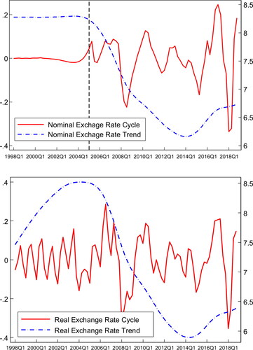
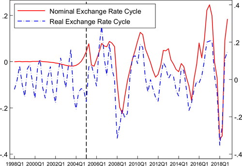
Figure 2. The co-movements of nominal and real-exchange rate cycles. The sample covers the period from 1998 to 2018, and the data are from IMF. Both nominal and real-exchange rate cycles are HP filtered (λ = 100) and expressed as percentage deviations from the trend. The real-exchange rate equals the nominal exchange rate multiplied by the U.S. CPI inflation rate (2010 = 100), and then divided by the China CPI inflation rate (2010 = 100). The nominal exchange rate is used with quarterly average data of one U.S. dollar to the Chinese RMB. In the figure, the red solid line is calibrated with the ordinate left axis, and the blue dotted line is calibrated with the ordinate right axis.

Most of the literature suggests that an increase in the U.S. nominal interest rate causes U.S. dollar appreciation and other currencies’ depreciation, which leads to the improvement of other countries' international trade, current account, and output (Christiano et al., 1996; Dedola et al., 2017; Devereux et al., 2019; Engel, 2016; Kim et al., 2017; Schmidt et al., 2018). However, some studies have recently found that the neo-Fisher effect exists.

Neo-Fisher effect is based on the Fisher effect to describe the short-term relationship between inflation rate and nominal interest rate. Permanent increases in nominal interest rates cause the immediate rise of inflation and decline of real-interest rates (Cochrane, 2016; Ioana, 2017; Uribe, 2018). García-Schmidt and Woodford (2019) suggest that the condition of the neo-Fisher effect is rational expectation, and argue that if the rational expectation is replaced by limited period planning, the existence of the neo-Fisher effect may not be supported. However, Uribe (2018) builds New-Keynesian theoretical model and SVAR empirical model to verify the existence of the neo-Fisher Effect in the United States and Japan.

Based on the neo-Fisher effect, Uribe and Schmitt-Grohé (2018) suggest that the permanent increase in the U.S. nominal interest rates causes U.S. inflation to rise, resulting in U.S. dollar depreciation against the British pound and the Japanese yen. The U.S. temporary increase in the nominal interest rate causes U.S. dollar appreciation. At the same time, De Michelis and Iacoviello (2016) suggest that a positive shock to Japan's inflation target causes Japanese yen depreciation.

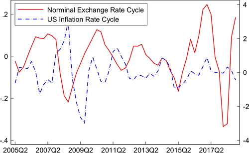
As depicted in Figure 3, there is a significant reverse co-movement between the bilateral nominal exchange rate and the U.S. inflation rate from 2005 to 2018. When the U.S. inflation rate rises, the bilateral nominal exchange rate declines, indicating depreciation in the U.S. dollar and appreciation in the Chinese yuan. When the U.S. inflation rate declines, the bilateral nominal exchange rate increases; that is, the U.S. dollar appreciates, and the Chinese yuan depreciates.

Figure 3. The co-movement fact between U.S. dollar-Chinese yuan nominal exchange rate and U.S. inflation rate. The sample covers the period from 2005 to 2018 and is from IMF. The nominal exchange rate and the U.S. inflation rate are HP filtered (λ = 100) and expressed as percentage deviations from the trend. The nominal exchange rate is used with quarterly average data of one U.S. dollar to the Chinese RMB. The U.S. inflation rate is the CPI inflation rate (2010 = 100), which is from the IMF. In the figure, the red solid line is calibrated with the ordinate left axis, and the blue dotted line is calibrated with the ordinate right axis.

The theoretical model developed in this study extends the work of Galí and Monacelli (2005), Smets and Wouters (2003) and Cochrane (2016) to consider the environment with U.S. permanent and temporary shocks. The empirical framework employs the SVAR model and Bayesian technique to evaluate the spillover impact of U.S. permanent and temporary monetary shocks. We obtain two main results. First, the permanent increase in the U.S. nominal interest rates causes U.S. inflation rate to rise, leading to Chinese yuan appreciation and U.S. dollar depreciation. The permanent increase in U.S. nominal interest rates has a negative spillover impact on China’s macroeconomy and results in its real-output declining through the exchange rate channel. Second, the temporary increase in U.S. nominal interest rates leads to depreciation in the Chinese yuan and appreciation in the U.S. dollar, which have a positive spillover impact on China’s macroeconomy and lead to an increase in its real output.

This paper proceeds as follows: Section 2 analyses the heterogeneity spillover impacts of U.S. permanent and temporary monetary shocks on China’s economy through the exchange rate channel with the New Keynesian transmission model. Section 3 presents the SVAR empirical model, describes the data used for estimation, and their sources. Section 4 presents the main findings of the SVAR empirical model. Section 5 closes and concludes the paper.

2. Two-country transmission model

In this section, we refer to existing literature (Cochrane, 2016; Galí and Monacelli, 2005; Smets and Wouters, 2003), to construct a new-Keynesian transmission model featuring price stickiness. The goal is twofold. One is to ascertain how the U.S. permanent monetary shocks produce neo-Fisher effects. The other is to analyse the heterogeneity spillover impacts of the U.S. permanent and temporary monetary shocks through the exchange rate channel from the perspective of new-Keynesian transmission model. Hamilton (1994) states that when the exogenous shock increases by one unit in the current period and then returns to the original level, the exogenous shock on endogenous variables is temporary. When exogenous shock increases by one unit during each period, the shock impact of permanent change from the current period on endogenous variables is a permanent shock.

Consider an open economy with two symmetric countries. One is the home country, and the other is the foreign country. The two countries share the same preferences and technologies. For convenience, we standardise the total number of households in the two countries as 1, with the proportion of domestic residents as θ, and the proportion of foreign residents as 1-θ. There is no movement of labour between countries. Households can consume both domestic and foreign final products and trade state-dependent portfolios in the international complete securities markets.

There are two types of companies in the two countries, which are the intermediate and final goods firms. The intermediate firms are monopolistic competitors that produce differentiated products for final goods firms. The final firms sell homogeneous products in the competitive market, and the profits belong to the households. Specifically, we assume that the number of final firms in the two countries equals the number of households. Suppose that there are no barriers to trade between countries. In addition, we assume the law of one price holds for every commodity.

2.1. Utility function and market structure

The home country has θ proportion of identical households, as described by the following utility function: (1) $$U_t=E_t\sum _{t=0}^{\infty }{\beta }^t\{\frac{C_t^{1-\sigma }}{1-\sigma }-\frac{N_t^{1+\eta }}{1+\eta }\}$$(1) where C_t denotes final goods consumption index and N_t denotes the hours worked. σ is the intertemporal substitution elasticity of consumption, and σ > 0. η is the intertemporal substitution elasticity of the working hour supply, and η > 0. Assume that the period utility function U is strictly increasing and strictly concave. The parameter β, denoting the subjective discount factor, ranges in the interval (0, 1). E_t denotes the mathematical expectations operator conditional on the available information in period t.

Assume that C_t is composed of domestic final goods consumption C_h,t and foreign final goods consumption C_f,t. (2) $$C_t\equiv C_{h,t}^{\theta }{C}_{f,t}^{1-\theta }$$(2) where 0<θ < 1. Suppose that the preferences of foreign families are symmetrical.

P_t denotes the corresponding consumption price index. P_h,t is the domestic price index of consumption goods, and P_f,t is the foreign price index of consumption goods. Given total consumption, and following cost minimization, we obtain the consumption price index as, (3) $$P_t={\omega }^{-1}{P}_{h,t}^{\theta }{P}_{f,t}^{1-\theta }$$(3) where ω = θ^θ(1-θ)^1-θ. Simultaneously, the proportion of households' consumption of domestic goods is θ and that of foreign goods is 1-θ. (4) $$P_{h,t}{C}_{h,t}=\theta P_t{C}_t$$(4) (5) $$P_{f,t}{C}_{f,t}=(1-\theta )P_t{C}_t$$(5)

As the law of one price holds for every commodity, we obtain $P_{f,t}={\epsilon }_t{P}_{h,t}={\epsilon }_t{P}_{f,t}^{\ast }$ and $P_{h,t}=P_{f,t}/{\epsilon }_t=P_{h,t}^{\ast }/{\epsilon }_t,$ where ε_t is the bilateral nominal exchange rate, which is defined as the price of foreign currency in domestic currency. $P_{f,t}^{\ast }$ is the domestic currency price of foreign final goods sold in the domestic market, and $P_{h,t}^{\ast }$ is the foreign currency price of domestic final goods sold in the foreign market. Then, we can rewrite the consumption price index function as (6). (6) $$P_t={\omega }^{-1}{P}_{h,t}{\epsilon }_t^{1-\theta }$$(6)

The corresponding foreign consumption price index function can be written as (2–7). (7) $$P_t^{\ast }={\omega }^{-1}{P}_{h,t}{\epsilon }_t^{-\theta }$$(7)

Combining (6) and (7), we obtain the law of one price holds for the consumption price index. (8) $$P_t={\epsilon }_t{P}_t^{\ast }$$(8)

Households have access to state-contingent portfolios. We let B_t+1(s) denote the portfolio purchased from households in the state of s in the period t, with bond price of Q_t+1(s). The household budget constraint equation is given by, (9) $$\sum _{s\in S}{Q}_{t+1}(s)B_{t+1}(s)+P_t{C}_t+{{\rm T}}_t=B_t+{\Gamma }_t+W_t{N}_t$$(9) where S denotes the set of states, T_t denotes a lump sum tax, and Γ_t denotes the profits acquired from the intermediate goods firms, and W_t denotes the nominal wage.

Given W_t, P_t, Q_t+1(s), T_t, Γ_t, households choose C_t, N_t, B_t+1 to maximise their utilities depicted in Equation (1)(1) $$U_t=E_t\sum _{t=0}^{\infty }{\beta }^t\{\frac{C_t^{1-\sigma }}{1-\sigma }-\frac{N_t^{1+\eta }}{1+\eta }\}$$(1) with the budget constraint Equation (9)(9) $$\sum _{s\in S}{Q}_{t+1}(s)B_{t+1}(s)+P_t{C}_t+{{\rm T}}_t=B_t+{\Gamma }_t+W_t{N}_t$$(9) . Let q_t+1(s) denote the possibility of state s in period t. (10) $$U_C(C_t)=C_t^{-\sigma }={\lambda }_t$$(10) (11) $$U_N(N_t)=N_t^{\eta }={\lambda }_t\frac{W_t}{P_t}$$(11)

For all $s\in S,$ we have, (12) $${\lambda }_t{E}_t\frac{Q_{t+1}(s)}{P_t}=\beta E_t\frac{{\lambda }_{t+1}(s)q_{t+1}(s)}{P_{t+1}}$$(12) where λ_t denotes the Lagrange multiplier related to the budget constraint Equation (9)(9) $$\sum _{s\in S}{Q}_{t+1}(s)B_{t+1}(s)+P_t{C}_t+{{\rm T}}_t=B_t+{\Gamma }_t+W_t{N}_t$$(9) .

Combining (10) and (11) yields (13) as follows: (13) $$\frac{U_N(N_t)}{U_C(C_t)}=\frac{N_t^{\eta }}{C_t^{-\sigma }}=\frac{W_t}{P_t}$$(13)

Function (13) shows that the optimal labour supply is obtained when the marginal substitution rate of leisure and consumption is the real wage rate of labour.

Combining (10) and (12) yields (14), (14) $$C_t^{-\sigma }{E}_t\frac{Q_{t+1}(s)}{P_t}=\beta E_t\frac{C_{t+1}^{-\sigma }(s)q_{t+1}(s)}{P_{t+1}}$$(14)

Then, sum up all the states $s\in S$ according to (14), and let $R_t=1/\sum _{s\in S}{Q}_{t+1}(s)$ denote the risk-free gross rate. (15) $$C_t^{-\sigma }=\beta R_t{E}_t\frac{P_t}{P_{t+1}}{C}_{t+1}^{-\sigma }$$(15)

Under the assumption of complete securities markets, households in each country can purchase state-contingent bonds in the international securities market to hedge consumption risk. A first-order condition analogous to (15) must also hold for foreign representative households. (16) $${(C_t^{\ast })}^{-\sigma }=\beta R_t{E}_t\frac{{\epsilon }_t{P}_t^{\ast }}{{\epsilon }_{t+1}{P}_{t+1}^{\ast }}{(C_{t+1}^{\ast })}^{-\sigma }$$(16) where $C_t^{\ast }$ denotes foreign consumption.

Combining (16), and the law of one price holds for the consumption price index $P_t={\epsilon }_t{P}_t^{\ast }.$ We obtain (17). (17) $$(C_t/C_t^{\ast })=(C_{t+1}/C_{t+1}^{\ast })$$(17)

Equation (17)(17) $$(C_t/C_t^{\ast })=(C_{t+1}/C_{t+1}^{\ast })$$(17) indicates that domestic and foreign consumption growth is equal at any time. Therefore, we have $C_t=\rho C_t^{\ast },$ and standardise ρ = 1. (18) $$C_t=C_t^{\ast }$$(18)

2.2. Firms

Assume that the final firms in the home country are produced with a continuum of varieties of intermediate goods according to the following CES technology: $$Y_t={\left[{\int }_0^1{y}_t{(z)}^{\frac{\gamma -1}{\gamma }}dz\right]}^{\frac{\gamma }{\gamma -1}}$$ where γ > 1. Y_t denotes the final goods output, and y_t(z) denotes the intermediate goods z produced by the intermediate firms. Both Y_t and y_t(z) are expressed in per capita terms. Each final goods firm takes the final goods price P_h,t and intermediate goods price p_h,t(z) as given and maximises its profit. Then, we obtain the domestic price index. (19) $$p_{h,t}(z)={\left[\frac{y_{h,t}(z)}{Y_t}\right]}^{-\frac{1}{\gamma }}{P}_{h,t}$$(19)

When the market is in equilibrium, the production profit of the final product is zero, so the price of the domestic final product can be expressed as (20). (20) $$P_{h,t}={\left[{\int }_0^1{p}_{h,t}{(z)}^{1-\gamma }dz\right]}^{\frac{1}{1-\gamma }}$$(20)

As assumed before, the intermediate firms use a linear technology, $$y_{h,t}(z)=A_t{N}_t$$ where A_t is an exogenous technology parameter. Intermediate goods firms choose a price p_h,t(z), to maximise their profit. (21) $$p_{h,t}(z)=\frac{\gamma }{\gamma -1}\frac{W_t}{A_t}$$(21)

As the right side of Equation (21)(21) $$p_{h,t}(z)=\frac{\gamma }{\gamma -1}\frac{W_t}{A_t}$$(21) has nothing to do with intermediate product z, and the price of each intermediate good is added to the nominal effective marginal cost W_t/A_t by γ/(γ-1). Thus, we obtain P_h,t=p_h,t(z)= [γ/(γ-1)] [W_t/A_t], and then the real effective marginal cost of each firm can be expressed by (22). (22) $$M{C}_t=\frac{W_t/P_{h,t}}{A_t}$$(22)

Combining Equations (6)(6) $$P_t={\omega }^{-1}{P}_{h,t}{\epsilon }_t^{1-\theta }$$(6) , (13), and (22), we can rewrite the domestic real-effective marginal cost by (23). (23) $$M{C}_t=\frac{N_t^{\eta }/C_t^{-\sigma }}{A_t}\frac{P_t}{P_{h,t}}=\frac{N_t^{\eta }/C_t^{-\sigma }}{\omega A_t}{\epsilon }_t^{1-\theta }$$(23)

Equation (23)(23) $$M{C}_t=\frac{N_t^{\eta }/C_t^{-\sigma }}{A_t}\frac{P_t}{P_{h,t}}=\frac{N_t^{\eta }/C_t^{-\sigma }}{\omega A_t}{\epsilon }_t^{1-\theta }$$(23) implies that when other factors remain unchanged, the bilateral nominal exchange rate rises, and the domestic real-effective marginal cost rises, which leads to an increase in the domestic price.

2.3. Equilibrium

In equilibrium, the goods market clearing in both the home and foreign countries, so we get, (24) $$\theta Y_t=\theta C_{h,t}+(1-\theta )C_{h,t}^{\ast }$$(24) (25) $$(1-\theta )Y_t^{\ast }=\theta C_{f,t}^{\ast }+(1-\theta )C_{f,t}$$(25)

Combining Equations (4)(4) $$P_{h,t}{C}_{h,t}=\theta P_t{C}_t$$(4) , (24) and (25), we obtain the following equations: (26) $$P_t{C}_t=P_{h,t}{Y}_t$$(26) (27) $$P_t^{\ast }{C}_t^{\ast }=P_{f,t}^{\ast }{Y}_t^{\ast }$$(27)

Then, combining equations (18)(18) $$C_t=C_t^{\ast }$$(18) , (27), and the law of one price equation, we obtain, (28) $$\frac{Y_t}{Y_t^{\ast }}=\frac{P_{f,t}}{P_{h,t}}={\epsilon }_t$$(28)

Multiply two sides of Equation (6)(6) $$P_t={\omega }^{-1}{P}_{h,t}{\epsilon }_t^{1-\theta }$$(6) with C_t, that is, $P_t^{\ast }{C}_t^{\ast }=P_{f,t}^{\ast }{Y}_t^{\ast }={\omega }^{-1}{P}_{h,t}{C}_t^{\ast }{\epsilon }_t^{-\theta }.$ Then, we obtain the domestic output equation. (29) $$Y_t={\omega }^{-1}{C}_t{\epsilon }_t^{1-\theta }$$(29)

In the same way, multiplying two sides of Equation (7)(7) $$P_t^{\ast }={\omega }^{-1}{P}_{h,t}{\epsilon }_t^{-\theta }$$(7) with $C_t^{\ast },$ that is $P_t^{\ast }{C}_t^{\ast }=P_{f,t}^{\ast }{Y}_t^{\ast }={\omega }^{-1}{P}_{h,t}{C}_t^{\ast }{\epsilon }_t^{-\theta },$ we obtain the foreign output equation. (30) $$Y_t^{\ast }={\omega }^{-1}{C}_t^{\ast }{\epsilon }_t^{-\theta }$$(30)

Hence, we relist the equilibrium conditions as follows: (31) $$C_t^{-\sigma }=\beta R_t{E}_t\frac{P_t}{P_{t+1}}{C}_{t+1}^{-\sigma }$$(31) (32) $${(C_t^{\ast })}^{-\sigma }=\beta R_t{E}_t\frac{{\epsilon }_t{P}_t^{\ast }}{{\epsilon }_{t+1}{P}_{t+1}^{\ast }}{(C_{t+1}^{\ast })}^{-\sigma }$$(32) (33) $$C_t=C_t^{\ast }$$(33) (34) $$Y_t={\omega }^{-1}{C}_t{\epsilon }_t^{1-\theta }$$(34)

2.4. Foreign monetary policy shocks

For convenience in producing our results, we linearise Equations (31)(31) $$C_t^{-\sigma }=\beta R_t{E}_t\frac{P_t}{P_{t+1}}{C}_{t+1}^{-\sigma }$$(31) , (34), and then obtain a linearised version of the model. (35) $$-\sigma {\widehat{C}}_t={\widehat{P}}_t-E_t{\widehat{P}}_{t+1}-\sigma E_t{\widehat{C}}_{t+1}+{\widehat{R}}_t$$(35) (36) $$-\sigma {\widehat{C}}_t^{\ast }={\widehat{P}}_t^{\ast }-E_t{\widehat{P}}_{t+1}^{\ast }-\sigma E_t{\widehat{C}}_{t+1}^{\ast }+{\widehat{R}}_t+{\widehat{\epsilon }}_t-E_t{\widehat{\epsilon }}_{t+1}$$(36) (37) $${\widehat{C}}_t={\widehat{C}}_t^{\ast }$$(37) (38) $${\widehat{Y}}_t={\widehat{C}}_t+(1-\theta ){\widehat{\epsilon }}_t$$(38) where we define ${\widehat{C}}_t\equiv d{C}_t/{\overline{C}}_0,$ ${\widehat{C}}_t^{\ast }\equiv d{C}_t^{\ast }/{\overline{C}}_0^{\ast },$ ${\widehat{P}}_t\equiv d{P}_t/{\overline{P}}_0,$${\widehat{P}}_t^{\ast }\equiv d{P}_t^{\ast }/{\overline{P}}_0^{\ast },$ ${\widehat{R}}_t\equiv d{R}_t/{\overline{R}}_0,$ ${\widehat{Y}}_t\equiv d{Y}_t/{\overline{Y}}_0.$

Combining (37), we obtain the relationship function of the bilateral nominal exchange rate and inflation rate. (39) $$E_t{\widehat{\epsilon }}_{t+1}-{\widehat{\epsilon }}_t=E_t{\widehat{\pi }}_{t+1}-E_t{\widehat{\pi }}_{t+1}^{\ast }$$(39) where we define $E_t{\widehat{\pi }}_{t+1}=E_t{\widehat{P}}_{t+1}-{\widehat{P}}_t,$ $E_t{\widehat{\pi }}_{t+1}^{\ast }=E_t{\widehat{P}}_{t+1}^{\ast }-{\widehat{P}}_{t+1}^{\ast }.$

Referring to Cochrane (2016), we assume that foreign monetary policy is subject to the discretion equations. $$y_t^{\ast }=E_t{y}_{t+1}^{\ast }-\varsigma (i_t^{\ast }-E_t{\pi }_{t+1}^{\ast })$$ $${\pi }_t^{\ast }=\nu E_t{\pi }_{t+1}^{\ast }+\kappa y_t^{\ast }$$ where parameters 災,ν,災 reside in the interval (0, 1). $y_t^{\ast }$ denotes the foreign output gap, $i_t^{\ast }$ and denotes the foreign policy rate. Introducing the lag operation L, we can rewrite the above equations as follows: (40) $$E_t(1-L^{-1})y_t^{\ast }=\varsigma E_t{L}^{-1}{\pi }_t^{\ast }-\varsigma i_t^{\ast }$$(40) (41) $$E_t(1-\nu L^{-1}){\pi }_t^{\ast }=\kappa y_t^{\ast }$$(41)

After solving the equations, we obtain the geometrically weighted distributed lags of the foreign inflation rate and interest rate path. (42) $${\pi }_{t+1}^{\ast }=\frac{\kappa \varsigma }{({\xi }_1-{\xi }_2)}(i_t^{\ast }+\sum _{j=1}^{\infty }{\xi }_1^{-j}{i}_{t-j}^{\ast }+\sum _{j=1}^{\infty }{\xi }_2^j{E}_{t+1}{i}_{t+j}^{\ast })+\sum _{j=0}^{\infty }{\xi }_1^{-j}{\chi }_{t+1-j}^{\ast }$$(42) where ${\chi }_{t+1}^{\ast }={\pi }_{t+1}^{\ast }-E_t{\pi }_{t+1}^{\ast }$ is a sequence of unpredictable random variables, and $E_t{\chi }_{t+1}^{\ast }=0.$ $${\xi }_1=[(1+\nu +\kappa \varsigma )+\sqrt{{(1+\nu +\kappa \varsigma )}^2-4}\nu ]/2>1,0<{\xi }_2=[(1+\nu +\kappa \varsigma )-\sqrt{{(1+\nu +\kappa \varsigma )}^2-4}\nu ]/2<1$$

Based on rational expectation, we linearise Equation (42)(42) $${\pi }_{t+1}^{\ast }=\frac{\kappa \varsigma }{({\xi }_1-{\xi }_2)}(i_t^{\ast }+\sum _{j=1}^{\infty }{\xi }_1^{-j}{i}_{t-j}^{\ast }+\sum _{j=1}^{\infty }{\xi }_2^j{E}_{t+1}{i}_{t+j}^{\ast })+\sum _{j=0}^{\infty }{\xi }_1^{-j}{\chi }_{t+1-j}^{\ast }$$(42) . (43) $$E_t{\widehat{\pi }}_{t+1}^{\ast }={\widehat{i}}_t^{\ast }+\sum _{j=1}^{\infty }{\widehat{i}}_{t-j}^{\ast }+\sum _{j=1}^{\infty }{E}_{t+1}{\widehat{i}}_{t+j}^{\ast }$$(43)

Hence, we rewrite the linearised version of Equations (43)(43) $$E_t{\widehat{\pi }}_{t+1}^{\ast }={\widehat{i}}_t^{\ast }+\sum _{j=1}^{\infty }{\widehat{i}}_{t-j}^{\ast }+\sum _{j=1}^{\infty }{E}_{t+1}{\widehat{i}}_{t+j}^{\ast }$$(43) , (39), and (38). (44) $$E_t{\widehat{\pi }}_{t+1}^{\ast }={\widehat{i}}_t^{\ast }+\sum _{j=1}^{\infty }{\widehat{i}}_{t-j}^{\ast }+\sum _{j=1}^{\infty }{E}_{t+1}{\widehat{i}}_{t+j}^{\ast }$$(44) (45) $$E_t{\widehat{\epsilon }}_{t+1}-{\widehat{\epsilon }}_t=E_t{\widehat{\pi }}_{t+1}-E_t{\widehat{\pi }}_{t+1}^{\ast }$$(45) (46) $${\widehat{Y}}_t={\widehat{C}}_t+(1-\theta ){\widehat{\epsilon }}_t$$(46)

According to Equation (44)(44) $$E_t{\widehat{\pi }}_{t+1}^{\ast }={\widehat{i}}_t^{\ast }+\sum _{j=1}^{\infty }{\widehat{i}}_{t-j}^{\ast }+\sum _{j=1}^{\infty }{E}_{t+1}{\widehat{i}}_{t+j}^{\ast }$$(44) , when a foreign country adopts a permanent nominal interest rate to adjust the macroeconomy, the foreign interest rate will rise from period t. Hence, the foreign inflation rate will immediately rise as well. It proves the existence of the neo-Fisher effect in the open economy. Equation (45)(45) $$E_t{\widehat{\epsilon }}_{t+1}-{\widehat{\epsilon }}_t=E_t{\widehat{\pi }}_{t+1}-E_t{\widehat{\pi }}_{t+1}^{\ast }$$(45) denotes when the domestic inflation rate remains unchanged and foreign inflation rate rises, the bilateral nominal exchange rate will decline; that is, domestic currency will appreciate and foreign currency will depreciate. Then, according to Equation (46)(46) $${\widehat{Y}}_t={\widehat{C}}_t+(1-\theta ){\widehat{\epsilon }}_t$$(46) , domestic currency appreciates result in domestic output declining. At this time, permanent rising in foreign nominal interest rates has a negative spillover effect on the domestic macroeconomy by the exchange rate channel.

When the foreign country adopts a temporary nominal interest rate to adjust the macroeconomy, the foreign interest rate rises in period t but returns to the original level in t + 1. Then, the foreign inflation rate may decline from period t + 1 onward. Assuming the domestic inflation rate remains unchanged, when the foreign inflation rate declines, the bilateral nominal exchange rate will rise, that is, domestic currency will depreciate and foreign currency will appreciate, resulting in a decline in domestic output. Hence, a temporary rise in the foreign nominal interest rate has a positive spillover effect on the domestic economy by the exchange rate channel. Therefore, the impact of the permanent and temporary increase in the U.S. nominal interest rate is heterogeneous through exchange rate channel.

3. The empirical model

3.1. SVAR model

Based on the theoretical model, we construct the SVAR empirical model to verify the heterogeneity spillover impacts of the U.S. permanent and temporary monetary shocks on China’s economy through exchange rate channel. Refer to Uribe (2018), Uribe and Schmitt-Grohé (2018), the SVAR model let the U.S. permanent monetary policy shock compete with the U.S. temporary monetary policy shock and with other shocks, from which the spillover effects of the U.S. permanent and temporary monetary policy shocks are obtained. The model has five shocks: the U.S. permanent monetary policy shock, denoted $X_t^{\mathit{mus}};$ the U.S. temporary monetary policy shock, denoted $z_t^{\mathit{mus}};$ as China permanent monetary policy shock, denoted $X_t^{\mathit{mchn}};$as permanent non-monetary policy shock, denoted $X_t^n;$ and temporary non-monetary policy shock, denoted $z_t^n.$

The model has five endogenous variables, which are assumed to be nonstationary. The logarithm of the real-domestic output y_t, which is assumed to be cointegrated with $X_t^n.$ U.S. nominal interest rate $i_t^{us}$ and U.S. inflation ${\pi }_t^{us}$ are assumed to be cointegrated with $X_t^{\mathit{mus}}.$ China’s nominal interest rate $i_t^{\mathit{mchn}}$ is assumed to be cointegrated with $X_t^{\mathit{mchn}}.$ The depreciation rate of the bilateral nominal exchange rate, e_t=ln(ε_t/ε_t-1), which is assumed to be cointegrated with $X_t^{\mathit{mchn}}-X_t^{\mathit{mus}}.$ ε_t denotes the nominal exchange rate, priced as one U.S. dollar in terms of China Yuan in period t. The five variables y_t, ${\pi }_t^{us},$ $i_t^{us},$ $i_t^{\mathit{chn}},$ e_t are expressed in percent per year.

We define the following vector of stationary variables, $$\left(\begin{array}{c}{\widehat{y}}_t\\ {\widehat{\pi }}_t^{us}\\ {\widehat{i}}_t^{us}\\ {\widehat{e}}_t\\ {\widehat{i}}_t^{\mathit{chn}}\end{array}\right)\equiv \left(\begin{array}{c}{y}_t-X_t^n\\ {\pi }_t^{us}-X_t^{\mathit{mus}}\\ i_t^{us}-X_t^{\mathit{mus}}\\ e_t-X_t^{\mathit{mchn}}+X_t^{\mathit{mus}}\\ i_t^{\mathit{chn}}-X_t^{\mathit{mchn}}\end{array}\right)$$ and assume that it evolves according to the following autoregressive process: (47) $$\left(\begin{array}{c}{\widehat{y}}_t\\ {\widehat{\pi }}_t^{us}\\ {\widehat{i}}_t^{us}\\ {\widehat{e}}_t\\ {\widehat{i}}_t^{\mathit{chn}}\end{array}\right)\equiv \sum _{i=1}^L{B}_i\left(\begin{array}{c}{y}_t-X_t^n\\ {\pi }_t^{us}-X_t^{\mathit{mus}}\\ i_t^{us}-X_t^{\mathit{mus}}\\ e_t-X_t^{\mathit{mchn}}+X_t^{\mathit{mus}}\\ i_t^{\mathit{chn}}-X_t^{\mathit{mchn}}\end{array}\right)+C\left(\begin{array}{c}\Delta X_t^{\mathit{mus}}\\ z_t^{\mathit{mus}}\\ \Delta X_t^n\\ z_t^n\\ \Delta X_t^{\mathit{mchn}}\end{array}\right)$$(47) where B_i for i = 1, 2, 3, …, L and C are 5 × 5 matrices of coefficients, and L denotes the number of lags. We assume that the five exogenous shocks subject to AR (1) processes in the following form: (48) $$\left(\begin{array}{c}\Delta X_{t+1}^{\mathit{mus}}\\ z_{t+1}^{\mathit{mus}}\\ \Delta X_{t+1}^n\\ z_{t+1}^n\\ \Delta X_{t+1}^{\mathit{mchn}}\end{array}\right)=\rho \left(\begin{array}{c}\Delta X_t^{\mathit{mus}}\\ z_t^{\mathit{mus}}\\ \Delta X_t^n\\ z_t^n\\ \Delta X_t^{\mathit{mchn}}\end{array}\right)+\psi \left(\begin{array}{c}{\epsilon }_{t+1}^1\\ {\epsilon }_{t+1}^2\\ {\epsilon }_{t+1}^3\\ {\epsilon }_{t+1}^4\\ {\epsilon }_{t+1}^5\end{array}\right)$$(48) where ${\epsilon }_{t+1}^i$ (i = 1,2,3,4,5) ∼ i.i.d. N (0, 1), ρ and ψ are 5 × 5 diagonal matrices of coefficients. We can rewrite Equations (47)(47) $$\left(\begin{array}{c}{\widehat{y}}_t\\ {\widehat{\pi }}_t^{us}\\ {\widehat{i}}_t^{us}\\ {\widehat{e}}_t\\ {\widehat{i}}_t^{\mathit{chn}}\end{array}\right)\equiv \sum _{i=1}^L{B}_i\left(\begin{array}{c}{y}_t-X_t^n\\ {\pi }_t^{us}-X_t^{\mathit{mus}}\\ i_t^{us}-X_t^{\mathit{mus}}\\ e_t-X_t^{\mathit{mchn}}+X_t^{\mathit{mus}}\\ i_t^{\mathit{chn}}-X_t^{\mathit{mchn}}\end{array}\right)+C\left(\begin{array}{c}\Delta X_t^{\mathit{mus}}\\ z_t^{\mathit{mus}}\\ \Delta X_t^n\\ z_t^n\\ \Delta X_t^{\mathit{mchn}}\end{array}\right)$$(47) and (48) as (49). (49) $${\xi }_{t+1}=F{\xi }_t+P{\epsilon }_{t+1}$$(49) where $${\xi }_t\equiv \left(\begin{array}{ccccc}{\widehat{Y}}_t& {\widehat{Y}}_{t-1}& \cdots & {\widehat{Y}}_{t-L+1}& u_t\end{array}\right)\prime$$ $${\widehat{Y}}_t=\left(\begin{array}{ccccc}{\widehat{y}}_t& {\widehat{\pi }}_t^{us}& {\widehat{i}}_t^{us}& {\widehat{e}}_t& {\widehat{i}}_t^{\mathit{chn}}\end{array}\right)\prime$$ $$u_t=\left(\begin{array}{ccccc}\Delta X_t^{\mathit{mus}}& z_t^{\mathit{mus}}& \Delta X_t^n& z_t^n& \Delta X_t^{\mathit{mchn}}\end{array}\right)\prime$$ $${\epsilon }_t=\left(\begin{array}{ccccc}{\epsilon }_t^1& {\epsilon }_t^2& {\epsilon }_t^3& {\epsilon }_t^4& {\epsilon }_t^5\end{array}\right)\prime$$

The systems (47) and (48) are unobservable because neither the detrended endogenous variables nor the shocks are observed. To estimate the model, we add equations linking the unobservable variables to variables with an empirical counterpart. The five observable variables are the real-output Δy_t, the U.S. real-interest rate ${\widehat{i}}_t^{us}-{\widehat{\pi }}_t^{us},$ change in the U.S. nominal interest rate $\Delta i_t^{us},$ change in the China nominal interest rate $\Delta i_t^{\mathit{chn}},$ and change in the bilateral nominal depreciation rate Δe_t. (50) $$\begin{array}{l}\Delta y_t={\widehat{y}}_t-{\widehat{y}}_{t-1}+\Delta X_t^n\\ r_t^{us}={\widehat{i}}_t^{us}-{\widehat{\pi }}_t^{us}\\ \Delta i_t^{us}={\widehat{i}}_t^{us}-{\widehat{i}}_{t-1}^{us}+\Delta X_t^{\mathit{mus}}\\ \Delta e_t={\widehat{e}}_t-{\widehat{e}}_{t-1}+\Delta X_t^{\mathit{mchn}}-\Delta X_t^{\mathit{mus}}\\ \Delta i_t^{\mathit{chn}}={\widehat{i}}_t^{\mathit{chn}}-{\widehat{i}}_{t-1}^{\mathit{chn}}+\Delta X_t^{\mathit{mchn}}\end{array}$$(50)

The variables on the left-hand sides of (50) are assumed to have measurement error. We also assume that the econometrician observes the vector O_t defined as (51). (51) $$O_t\equiv \left(\begin{array}{c}\Delta y_t\\ r_t^{us}\\ \Delta i_t^{us}\\ e_t\\ \Delta i_t^{\mathit{chn}}\end{array}\right)+{\mu }_t$$(51) where μ_t is a 5 × 1 vector of measurement errors distributed i.i.d. N (∅, R), and R is a 5 × 5 diagonal variance-covariance matrix. Then, we can rewrite the system (50) and (51) as (52). (52) $$O_t=A^{\prime }+H^{\prime }{\xi }_t$$(52) where $$A^{\prime }\equiv \left(\begin{array}{ccccc}E(\Delta X_t^n)& E(i_t^{\mathit{mus}}-{\pi }_t^{us})& E(\Delta X_t^{\mathit{mus}})& E(\Delta X_t^{\mathit{mchn}}-\Delta X_t^{\mathit{mus}})& E(\Delta X_t^{\mathit{mchn}})\end{array}\right)\prime$$ $$H^{\prime }=\left(\begin{array}{ccc}{M}_{\xi }& {{\rm O}}_{5,5(L-2)}& M_u\end{array}\right)\prime$$ $$M_{\xi }=\left(\begin{array}{cccccccccc}1& 0& 0& 0& 0& -1& 0& 0& 0& 0\\ 0& -1& 1& 0& 0& 0& 0& 0& 0& 0\\ 0& 0& 1& 0& 0& 0& 0& -1& 0& 0\\ 0& 0& 0& 1& 0& 0& 0& 0& -1& 0\\ 0& 0& 0& 0& 1& 0& 0& 0& 0& -1\end{array}\right)$$ $$M_u=\left(\begin{array}{ccccc}0& 0& 1& 0& 0\\ 0& 0& 0& 0& 0\\ 1& 0& 0& 0& 0\\ -1& 0& 0& 0& 1\\ 0& 0& 0& 0& 1\end{array}\right)$$

3.2. Identification

We adapt the sign restriction approach to identify U.S. permanent and transitory monetary shocks, referring to Uribe and Schmitt-Grohé (2018). Specifically, we assume that temporary increases in the U.S. nominal interest rate have a positive effect on China’s output. We impose the sign restrictions of C₁₂ > 0 on the coefficients of matrix C in Equation (47)(47) $$\left(\begin{array}{c}{\widehat{y}}_t\\ {\widehat{\pi }}_t^{us}\\ {\widehat{i}}_t^{us}\\ {\widehat{e}}_t\\ {\widehat{i}}_t^{\mathit{chn}}\end{array}\right)\equiv \sum _{i=1}^L{B}_i\left(\begin{array}{c}{y}_t-X_t^n\\ {\pi }_t^{us}-X_t^{\mathit{mus}}\\ i_t^{us}-X_t^{\mathit{mus}}\\ e_t-X_t^{\mathit{mchn}}+X_t^{\mathit{mus}}\\ i_t^{\mathit{chn}}-X_t^{\mathit{mchn}}\end{array}\right)+C\left(\begin{array}{c}\Delta X_t^{\mathit{mus}}\\ z_t^{\mathit{mus}}\\ \Delta X_t^n\\ z_t^n\\ \Delta X_t^{\mathit{mchn}}\end{array}\right)$$(47) . We normalise the impact the innovation of a temporary non-monetary shock on China’s real output to unity, that is C14 = 1.

3.3. Estimation

We estimate the model quarterly using Bayesian techniques. We use the VAR lag order test for five endogenous variables, and subject to most rules as shown in Table 1, we set two lags in Equation (47)(47) $$\left(\begin{array}{c}{\widehat{y}}_t\\ {\widehat{\pi }}_t^{us}\\ {\widehat{i}}_t^{us}\\ {\widehat{e}}_t\\ {\widehat{i}}_t^{\mathit{chn}}\end{array}\right)\equiv \sum _{i=1}^L{B}_i\left(\begin{array}{c}{y}_t-X_t^n\\ {\pi }_t^{us}-X_t^{\mathit{mus}}\\ i_t^{us}-X_t^{\mathit{mus}}\\ e_t-X_t^{\mathit{mchn}}+X_t^{\mathit{mus}}\\ i_t^{\mathit{chn}}-X_t^{\mathit{mchn}}\end{array}\right)+C\left(\begin{array}{c}\Delta X_t^{\mathit{mus}}\\ z_t^{\mathit{mus}}\\ \Delta X_t^n\\ z_t^n\\ \Delta X_t^{\mathit{mchn}}\end{array}\right)$$(47) , L = 2. We follow Uribe and Schmitt-Grohé (2018) to assign the prior distributions of the estimated parameters in the model, which are shown in Table 2. Specifically, as most studies have proposed that an increase in U.S. interest rates has a negative effect on other countries’ economies, we impose a prior mean of 1 to the parameter C₂₁. We build a Monte-Carlo Markov chain (MCMC) of one million draws and burn the initial 0.1 million draws to obtain the posterior means and standard deviation of parameters listed in Table 3.

Table 1. Var lag order test.

Lag order	FPE	AIC	HQIC	SBIC
0	0.05169	11.2268	11.2992	11.4162
1	0.0100	9.5787	10.0130	10.7151*
2	0.0052*	8.8886*	9.6847*	10.9719
3	0.0083	9.2849	10.4428	12.3152
4	0.0075	9.0421	10.5619	13.0194

Table 2. Prior distributions of parameters.

Parameters	Distribution	Mean.	Std. Dev.
Main diagonal elements in B1	Normal	0.95	0.5
All other elements in B1, B2	Normal	0	0.25
C21, C31, C55	Normal	−1	1
C12, - C22	Gamma	1	1
All other elements of C	Normal	0	1
Ψ	Gamma	1	1
ρ11, ρ22, ρ33, ρ55	Beta	0.3	0.2
ρ44	Beta	0.7	0.2
A	Normal	mean(Ot)	$\sqrt{\mathit{Var}(O_t)/T}$
Rii, i = 1……5	Uniform [0,Var(Ot)/10]	Var(Ot)/(10*2)	Var(Ot)/(10*$\sqrt{12}$)

Table 3. Posterior means and standard deviation.

B1	Mean	0.8285	0.0137	0.2600	−0.2907	−0.0217
		0.2744	0.1900	0.3632	−0.3828	−0.2637
		0.0507	−0.0098	0.8429	0.2098	0.0191
		0.2100	0.1067	−0.0981	0.6670	−0.1238
		0.1002	−0.0063	−0.0502	0.0848	1.0423
	Std	0.0665	0.0247	0.0632	0.0610	0.0881
		0.1103	0.0620	0.1193	0.0963	0.0855
		0.0494	0.0213	0.0492	0.0522	0.0926
		0.0907	0.0643	0.0943	0.1099	0.0993
		0.0446	0.0155	0.0394	0.0480	0.0716
B2	Mean	−0.0312	−0.0576	−0.1737	0.1167	−0.3193
		−0.0287	−0.4850	0.1588	−0.1317	−0.4573
		−0.1831	−0.0035	0.1532	−0.1689	−0.1157
		−0.1553	−0.0415	−0.3110	0.0373	−0.0183
		−0.0213	−0.0101	0.0739	−0.0282	−0.2302
	Std	0.0658	0.0226	0.0616	0.0646	0.1039
		0.1351	0.0790	0.1061	0.1021	0.1011
		0.0590	0.0162	0.0506	0.0547	0.0843
		0.0900	0.0474	0.0957	0.0634	0.1005
		0.0487	0.0117	0.0471	0.0412	0.0719
C	Mean	−0.0846	1.2780	−0.9378	/	−0.4873
		0.8674	−0.1227	1.1683	0.7599	−1.1433
		−0.9118	/	0.0893	0.5737	0.3578
		−0.4187	1.1898	0.7135	−1.7299	0.4189
		0.0374	−0.9701	0.0000	0.6677	−0.8792
	Std	0.0461	0.1335	0.0383	/	0.1131
		0.1115	0.1062	0.0880	0.1500	0.1265
		0.0332	/	0.0248	0.0910	0.0914
		0.1077	0.2233	0.1042	0.1395	0.1268
		0.0261	0.1243	0.0226	0.1021	0.0878
ψ	Mean	0.8795	0.0612	1.0617	0.1968	0.2699
	Std	0.0733	0.0123	0.0877	0.0270	0.0467
ρ	Mean	0.0425	0.2268	0.0872	0.3796	0.1624
	Std	0.0318	0.1019	0.0591	0.1173	0.0986
A’	Mean	2.1311	−0.4814	0.0068	0.0498	−0.0132
	Std	0.0683	0.1050	0.0361	0.0608	0.0252
R	Mean	0.0157	0.1080	0.0046	0.0690	0.0022
	Std	0.0128	0.0931	0.0034	0.0626	0.0017

3.4. The data

The estimation uses quarterly data convers from the first quarter of 2005 to the fourth quarter of 2018. China’s real-output y_t adopts value-added GDP and is seasonally adjusted. The source is frbatlanta.org. The U.S. inflation rate ${\pi }_t^{us}$ is proxied by the growth rate of the U.S. consumer price index. The source is the IMF IFS database Consumer Price Index, all items, index 2010 = 100. The U.S. nominal interest rate $i_t^{us}$ is adopted with the U.S. federal funds rate (quarterly averages of monthly rates). The source is federalreserve.gov. China nominal interest rate $i_t^{\mathit{chn}}$ is proxied by the three-month deposit rate. The source is frbatlanta.org. The devaluation rate, is measured by the growth rate of the dollar-RMB nominal exchange rate (RMB price of one US dollar). The source is the IMF IFS database.

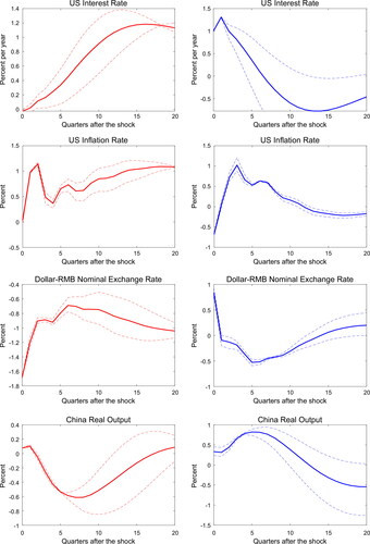
4. Impulse response analysis

Figure 4 displays the impulse response of the permanent and temporary increase in U.S. nominal interest rate shocks. The impulse response of the permanent increase in the U.S. nominal interest rate shocks is displayed in the left column of the figure. The impulse response of the temporary increase in U.S. nominal interest rate shocks is displayed in the right column of the figure. The results show the heterogeneity spillover impact of the U.S. permanent and temporary monetary policy on China’s economy.

Figure 4. Impulse responses to permanent and transitory U.S. monetary shocks.

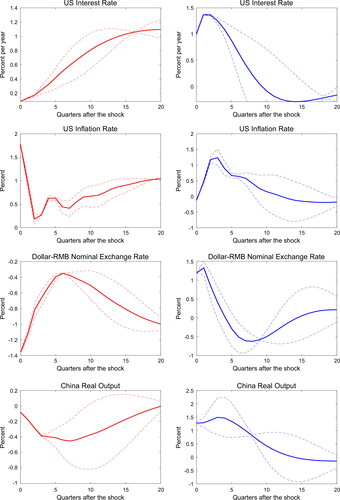
The permanent increase in the U.S. nominal interest rate by one unit produces the U.S. inflation rate rising immediately by more than one unit, which confirms the neo-Fisher effect in the open economy frame, similar to Uribe (2018). Hence, the bilateral nominal exchange rate shows an immediate decline by about 1.3% after the U.S. permanent monetary shock, which indicates U.S. dollar depreciation and China RMB appreciation. This result in a decline in China’s real output. Therefore, the permanent increase in U.S. nominal interest rate shocks has a negative spillover impact on China’s economy through the exchange rate channel.

In contrast, the temporary increase in the U.S. nominal interest rates leads to the bilateral nominal exchange rate rising immediately by approximately 1.25%, that is, U.S. dollar appreciation and China RMB depreciation. This result in an increase in China’s real output. Therefore, the temporary increase in U.S. nominal interest rate shocks has a positive spillover impact on China’s economy through the exchange rate channel.

The results remain unchanged when the nominal exchange rate is replaced with the real-exchange rate, as shown in Figure 5. The real exchange rate is calculated as the nominal exchange rate multiplied by the U.S. CPI index (2010 = 100) and divided by the China CPI index (2010 = 100) in period t. The source of the U.S. CPI index and China CPI index is the IMF IFS database.

Figure 5. Impulse responses to permanent and transitory U.S. monetary shocks.

From the impulse response shown in Figure 5, we find that the permanent increase in the U.S. nominal interest rate shocks leads to a bilateral real-exchange rate depreciating immediately by approximately 1.6%, declining more than the bilateral nominal exchange rate. In contrast, faced by the temporary increase in the U.S. nominal interest rate shocks, the bilateral real-exchange rate appreciates immediately by approximately 0.8%, rising less than the nominal exchange rate. Therefore, we obtain similar results through nominal and real-exchange rate channel tests. The permanent increase in U.S. nominal interest rate shocks has a negative spillover impact on China’s economy through the exchange rate channel. The temporary increase in U.S. nominal interest rate shocks has a positive spillover impact on China’s economy through the exchange rate channel.

4.1. Variance decomposition

Table 4 shows the variance decomposition of the five endogenous variables of the SVAR model to the five exogenous shocks. The U.S. permanent monetary shock is estimated to be an important spillover driver of China’s real output through the exchange rate channel. The permanent change in the U.S. nominal interest rate explains 31.34% of the change in the U.S. nominal interest rate, 38.41% of the change in U.S. inflation rate, 58.46% of the change in bilateral nominal exchange rate, 12.34% of the change in China’s nominal interest rate, and 11.99% of the change in China's real output.

Table 4. Forecast error variance decomposition.

Shocks	China’s real output	$\Delta {\pi }_t={\pi }_t-{\pi }_{t-1}\Delta y_t$ U.S. inflation rate	U.S. nominal interest rate	Nominal exchange rate	China nominal interest rate
U.S. permanent monetary shock	11.99	38.41	31.34	58.46	12.34
U.S. temporary monetary shock	1.40	0.06	2.56	0.34	6.25
Permanent nonmonetary shock	59.29	57.20	42.99	30.54	30.22
Temporary nonmonetary shock	16.73	0.90	12.93	4.93	28.80
China permanent monetary shock	10.58	3.43	10.17	5.73	22.38

Notes: The variance decomposition of the SVAR model is based on the results of the nominal exchange rate.

In contrast, the temporary change in U.S. monetary shocks plays a much smaller role than the permanent monetary shock. The temporary change in the U.S. nominal interest rate explains 2.56% of the change in the U.S. nominal interest rate, 0.06% of the change in the U.S. inflation rate, 0.34% of the change in the bilateral nominal exchange rate, 6.25% of the change in China’s nominal interest rate, and 1.4% of the change in China's real output.

The majority of studies in the spillover impact of the U.S. Monetary Policy shocks focus on the study of the U.S. temporary monetary shock, and argue that a temporary increase in the U.S. nominal interest rate causes the U.S. dollar appreciates, which has a positive spillover impact on the domestic economy. This study separates the U.S. permanent monetary policy shock from the U.S. temporary monetary policy shock, and obtains that the permanent increase in the U.S. nominal interest rate shocks have greater negative spillover impact on China’s economy through exchange rate channel. This result calls for paying more attention on the U.S. permanent monetary policy shocks.

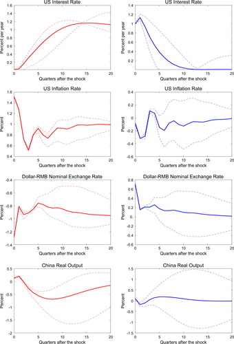
4.2. Robustness check

We first use the U.S. long-term nominal rate to replace the U.S. federal benchmark rate to perform a robustness test, as shown in Figure 6. The data source of the U.S. long-term interest rate is from OECD (https://data.oecd.org/). Then, we use the U.S. shadow rate and real-exchange rate to replace the federal funds rate and nominal exchange rate from the benchmark model and perform another robustness check, as shown in Figure 7. Both robustness test results are consistent with our suggestion. The permanent and temporary increase in the U.S. nominal interest rate shocks have a heterogeneous spillover impact on China’s economy through the exchange rate channel. The permanent increase in U.S. nominal interest rate shocks has a negative spillover impact on China’s economy through the exchange rate channel. The temporary increase in U.S. nominal interest rate shocks has a positive spillover impact on China’s economy through the exchange rate channel.

Figure 6. Impulse responses to permanent and temporary U.S. monetary shocks: robustness check 1.

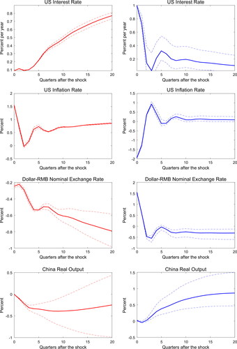
Figure 7. Impulse responses to permanent and temporary U.S. monetary shocks: robustness check 2.

5. Conclusion

Existing literature has suggested that a monetary shock that increases foreign interest rate shocks causes domestic currency depreciation both in nominal and real terms, which have a positive spillover impact on the domestic economy. In this study, we first construct the New Keynesian model to analyse the spillover impact of foreign permanent and temporary monetary shocks on the domestic economy through the exchange rate channel. This results in the heterogeneity spillover effect.

Then, we build the SVAR empirical model and separate the U.S. permanent monetary shocks from U.S. temporary monetary shocks. We confirm the heterogeneity spillover effects of the U.S. permanent and temporary monetary shocks on China’s economy through the exchange rates channel. First, the permanent increase in the U.S. nominal interest rate results in the U.S. inflation rate rising immediately, which fits the neo-Fisher effect referred to by Cochrane (2016) and Uribe (2018). Second, the permanent increase in the U.S. nominal interest rate shocks depreciates the U.S. dollar and appreciates the Chinese yuan in the short run, which resulted in the decline of China’s real output. The permanent increase in U.S. nominal interest rate shocks has a negative spillover impact on China’s economy through the exchange rate channel. The U.S. permanent monetary shocks explain an important fraction of the bilateral exchange rate and China’s real output.

Third, the temporary increase in the U.S. nominal interest rate shocks appreciate the U.S. dollar and depreciate the Chinese yuan in the short run, which results in the decline of China’s real output. The temporary increase in the U.S. nominal interest rate shock has a positive spillover impact on China’s economy through the exchange rate channel. However, U.S. temporary monetary shocks play a minor role in the exchange rate and spillover impact on China’s economy.

Generally, the adjustment of monetary policy of the Federal Reserve is usually a continuous increase or decrease in the nominal interest rate. As described in Uribe (2021), in the 1970s and 1980s, the high inflations coincided with the high levels of the nominal interest rate in the U.S. The theoretical and empirical results of this study show that the rise of the U.S. permanent nominal interest rate will lead to Chinese yuan appreciation and the decline of China's real output, the rise of the U.S. permanent nominal interest rate shock has a great negative spillover effect on China’s economy through the exchange rate channel. Chinese policy makers need to pay more attention to the permanent change of the U.S. monetary policy.

Acknowledgements

The authors thank Martin Uribe for sharing the code used in Uribe (2018). This study is the result of teamwork. All authors equally contributed in the study. Authors are ranked alphabetically by author’s last name.

Disclosure statement

No potential competing interest was reported by the authors.

References

- Aizenman, J., Chinn, M. D., & Ito, H. (2016). Monetary policy spillovers and the trilemma in the new normal: Periphery country sensitivity to core country conditions. Journal of International Money and Finance, 68, 298–330. https://doi.org/10.1016/j.jimonfin.2016.02.008
- Albagli, E., Ceballos, L., Claro, S., & Romero, D. (2019). Channels of US monetary policy spillovers to international bond markets. Journal of Financial Economics, 134(2), 447–473. https://doi.org/10.1016/j.jfineco.2019.04.007
- Baxter, M., & Stockman, A. C. (1989). Business cycles and the exchange rate regime: Some international evidence. Journal of Monetary Economics, 23(3), 377–400. https://doi.org/10.1016/0304-3932(89)90039-1
- Bräuning, F., & Ivashina, V. (2020). U.S. monetary policy and emerging market credit cycles. Journal of Monetary Economics, 112(1), 57–76. https://doi.org/10.1016/j.jmoneco.2019.02.005
- Cerutti, E., Claessens, S., & Puy, D. (2019). Push factors and capital flows to emerging markets: Why knowing your lender matters more than fundamentals. Journal of International Economics, 119, 133–149. https://doi.org/10.1016/j.jinteco.2019.04.006
- Christiano, L. J., Eichenbaum, M., & Evans, C. (1996). The effects of monetary policy shocks: Evidence from the flow of funds. The Review of Economics and Statistics, 78(1), 16–34. https://doi.org/10.2307/2109845
- Cochrane, J. H. (2016). Do higher interest rates raise or lower inflation? [Chicagobooth Research Paper], 1–91.
- Cushman, D. O., & Zha, T. (1997). Identifying monetary policy in a small open economy under flexible exchange rates. Journal of Monetary Economics, 39, 433–448.
- Dajčman, S., Kavkler, A., Mikek, P., & Romih, D. (2020). Transmission of financial stress shocks between the USA and the Euro area during different business cycle phases. E&M Economics and E + M Ekonomie a Management, 23(4), 152–165. https://doi.org/10.15240/tul/001/2020-4-010
- De Michelis, A., & Iacoviello, M. (2016). Raising an inflation target: The Japanese experience with Abenomics. European Economic Review, 88(2), 67–87. https://doi.org/10.1016/j.euroecorev.2016.02.021
- Dedola, L., Rivolta, G., & Stracca, L. (2017). If the Fed sneezes, who catches a cold? Journal of International Economics, 108, S23–S41. https://doi.org/10.1016/j.jinteco.2017.01.002
- Devereux, M. B., Dong, W., & Tomlin, B. (2019). Trade flows and exchange rates: Importers, exporters and products [NBER Working Paper, 26314].
- Engel, C. (2016). Exchange rates, interest rates, and the risk premium. American Economic Review, 106(2), 436–474. https://doi.org/10.1257/aer.20121365
- Flood, R. P., & Rose, A. K. (1995). Fixing exchange rate: A virtual quest for fundamentals. Journal of Monetary Economics, 36(1), 3–37. https://doi.org/10.1016/0304-3932(95)01210-4
- Fratzscher, M. (2012). Flows, push versus pull factors and the global financial crisis. Journal of International Economics, 88(2), 341–356. https://doi.org/10.1016/j.jinteco.2012.05.003
- Galí, J., & Monacelli, T. (2005). Monetary policy and exchange rate volatility in a small open economy. Review of Economic Studies, 72(3), 707–734. https://doi.org/10.1111/j.1467-937X.2005.00349.x
- García-Schmidt, M., & Woodford, M. (2019). Are low interest rates deflationary? A paradox of perfect-foresight analysis. American Economic Review, 109(1), 86–120. https://doi.org/10.1257/aer.20170110
- Hamilton, J. D. (1994). Time series analysis. Princeton University Press.
- Ioana, P. (2017). Monetary policy and inflation: Is there a Neo-Fisher effect? Evidence from inflation targeting countries in Central and Eastern Europe. Ovidius’ University Annals, Economic Sciences Series, 17(1), 578–583.
- Kim, S. (2001). International transmission of U.S. Monetary policy shocks: Evidence from VAR’s. Journal of Monetary Economics, 48(2), 339–372. https://doi.org/10.1016/S0304-3932(01)00080-0
- Kim, S.-H., Moon, S., & Velasco, C. (2017). Delayed overshooting: Is it an 1980s puzzle? Journal of Political Economy, 125(5), 1570–1598. https://doi.org/10.1086/693372
- Mussa, M. (1986). Nominal exchange rate regimes and the behavior of real exchange rates: Evidence and implications. Carnegie-Rochester Conference Series on Public Policy, 25, 117–214. https://doi.org/10.1016/0167-2231(86)90039-4
- Schmidt, J., Caccavaio, M., Carpinelli, L., & Marinelli, G. (2018). International spillovers of monetary policy: Evidence from France and Italy. Journal of International Money and Finance, 89, 50–66. https://doi.org/10.1016/j.jimonfin.2018.08.011
- Smets, F., & Wouters, R. (2003). An estimated dynamic stochastic general equilibrium model of the Euro area. Journal of the European Economic Association, 1(5), 1123–1175. https://doi.org/10.1162/154247603770383415
- Uribe, M. (2018). The Neo-Fisher effect: Econometric evidence from empirical and optimizing models [NBER Working paper, 25089].
- Uribe, M. (2021). The Neo-Fisher effect: Econometric evidence from empirical and optimizing models. American Economic Journal: Macroeconomics, forthcoming.
- Uribe, M., & Schmitt-Grohé, S. (2018). Exchange rates and uncovered interest differentials: The role of permanent monetary shocks [NBER Working paper, 25380].