Implications of macroeconomic conditions on Romanian portfolio credit risk. A cost-sensitive ensemble learning methods comparison

Abstract

Credit risk assessment represents a key instrument in the decision-making of the banking and financial institutions. In this article, we present a framework for credit risk strategies to improve portfolio efficiency under a change of macroeconomic regime. The aim is to compare the accuracy of several ensemble methods (AdaBoost, Logit Boost, Gentle Boost and Random Forest) on a default retail Romanian loan portfolio under different risk adversity scenarios, a priori and posteriori the financial distress. Using cost-sensitive ensemble learning models, we concluded that regime-based credit strategy can offer a better alternative in both terms of loss allocated to the strategy as well as defaulters’ classification accuracy.

Keywords:

• Credit policy
• financial distress
• risk aversion
• boosting
• random forest

JEL Classification:

• E44
• G21
• G32
• C55

1. Introduction

Credit risk assessment represents a key instrument in the decision-making of the banking and financial institutions. As Chen et al. (2020) pointed out credit risk has long been a pivotal problem of risk management in financial industry. This is why not only that it measures credit risk, but because any small improvement would produce great profits (Hand & Henley, 1997). In other words, the advantages of building a credible risk assessment are reducing the cost of credit analysis, ensuring fast decision-making, guaranteeing credit collection and reducing possible risks (Huang et al., 2018).

The analysis of credit risk has become more essential since the subprime mortgage crisis that began in 2007. A key feature of this financial distress is that in many countries worldwide the recovery in aggregate output has not been accompanied by a contemporary pick-up in bank lending flows, rendering the recovery credit-less. Behavioural factors of credit risk holders and financial market regulators have important effects on credit risk contagion (Chen et al., 2016). The disruption of bank lending following that financial distress resulted in sharp output contractions in both emerging and advanced economies (Corrado & Rossi, 2019). Indeed, people realised that one of the main causes of that crisis was that loans were granted to people whose risk profile was in reality too risky. That is why, in order to restore trust in the finance system and to prevent this from happening again, banks and other credit companies have tried to develop new models to assess the credit risk of individuals more accurately (Charpignon et al., 2014). Therefore, a range of different statistical and artificial intelligence methods have been developed to support credit decisions.

When considering credit risk assessment, we define a default profile to be considered as benchmark for the detection of the future profiles. As a perfect model would mean to detect both defaulters and non-defaulters and the objective is only one, the problem remains on what misclassification to penalise more. The cost of accepting a defaulter is far greater than the cost of rejecting a good applicant. One has to choose to maximise the overall accuracy and accept many defaults by setting a high cut-off or to minimise the average misclassification cost and reduce the acceptance rate. The first solution involves capital losses while the second one is related to market share therefore the challenge is to establish the precise costs in order to balance it. A cut-off point tuning process allows the credit policy makers to take cost-sensitive decision under different scenarios of uncertainty. The challenge is to train the data on a sample and obtain fairly good results on the test data having in mind a high accuracy through a low misclassification cost.

Regarding the credit risk assessment, recent studies have shown that machine learning techniques such as decision trees shows a better performance than a logistic model (Huang et al., 2018). According to the same authors, machine learning techniques do not require the assumption of variable distribution and can acquire knowledge directly from training data sets. Furthermore, artificial intelligence models perform better than the statistical ones especially when the credit risk assessment is a nonlinear model classification (Huang et al., 2018). The novelty of these methodologies relies on the power of the models to train the data. A simple decision tree will give the same result on a specific training data set as the learning is happening once. Building an ensemble of trees means to train different classifiers and use the most voted case, reaching better results as it is unlikely that all classifiers will make the same error. Among the ensemble models, gradient boosting decision tree and its variant algorithms have been applied as a homogeneous model itself or as a critical component of heterogeneous ensemble structure (Ma et al., 2018; Xia et al., 2018a, 2018b, 2020a, 2020b). Traditional credit risk models focus only on classification error rates and the different classification errors are assumed to attract the same costs. However, this is unrealistic, there is an inherent cost-sensitive problem in the credit risk assessment (Shen et al., 2019). Specifying a misclassification cost implies that the prior probabilities are adjusted for the weak learners.

In this paper, we will study the importance of cost-sensitive ensemble methods (AdaBoost, Logit Boost, Gentle Boost and Random Forest) in credit risk strategy selection when a shift in the default profile occurs. The change in the regime is captured by training cost-sensitive ensemble models on two different retail loan datasets. The Regime I data sample contains socio-demographic and financial data on defaulters prior the financial distress from 2008 and the second Regime is represented by the defaults that occurred after the structural break. The aim is to use the cost-sensitive ensemble methods (AdaBoost, Logit Boost, Gentle Boost and Random Forest) on training retail loan default data when changes have occurred. As misclassification costs behave as prior probabilities, the role of applying on the two regimes data is to underline the importance of training data set in establishing the risk strategies.

The remainder of the paper is extended as follows. Section 2 provides a brief review of the related literature. Section 3 describes the methodology. Section 4 describes the data used in the research and presents the empirical results and discussions. Section 5 concludes the study.

2. Literature review

Given the importance of the credit risk assessment in the decision-making of the banking and financial institutions, this subject is highly discussed within the literature and a large number of papers regarding all kinds of topics related to credit risk have been published.

Some papers focus more on the relation between macroeconomic conditions and credit quality. For example, Barra and Ruggiero (2021) investigated the effect of macroeconomic factors on bank credit risk and assessed how the 2008 financial distress affected the contribution of these factors to bank credit risk. The authors obtained that the financial distress determined an increase in banks’ credit rationing and the fact that macroeconomic factors have a significant effect. Colak and Senol (2021) examined the lending dynamics of banks in Turkey during various phases of the business cycle. According to the authors, public banks play a stabilising role when financial conditions tighten or the economy overheats, while domestic private and foreign banks’ lending behaviour is procyclical with the economic activity. Chortareas et al. (2020) focussed on the link between macroeconomic environment and credit risk, highlighting the idea that data characteristics, model specification, geographical distribution and time span of the sample are significant determinants in explaining the observed heterogeneity of the reported estimates in the literature. Kjosevski et al. (2019) explored and confirmed that macroeconomic determinants have an impact on the amount of non-performing loans to enterprises and households in the Republic of Macedonia. Allen et al. (2017) examined the relationship between bank lending, crises and changing ownership structure in Central and Eastern European countries and found that the influence of ownership structures on lending behaviours depends on the type of crisis that bank experience.

Other papers focus more on the methodology used to assess the credit risk. For example, Trivedi (2020) analysed credit scoring modelling on German credit data using machine learning approaches and found that Random Forest is the best among Bayesian, Naïve Bayes, Random Forest, Decision Tree and Support Vector Machine.

Zelenkov (2019) presented an example-dependent cost-sensitive generalisation of AdaBoost, testing the model on three synthetic data sets, as well as on two real problems of bank marketing and auto insurance. The results of the experiment proved that the proposed generalisation of AdaBoost outperformed other algorithms. In the author's opinion, AdaBoost outperforms other algorithms because it trains an ensemble of weak classifiers moving in the direction of the negative gradient to the loss function. Saidi et al. (2018) compared the performance of different cost-sensitive and cost-insensitive ensemble algorithms in determining the creditworthiness of private individuals. They found that the ensemble learning methods obtain better results than individual classifier, the insensitive approaches reached the best classification accuracy but to a trade-off. The models were not able to detect insolvent cases as the portfolio is highly imbalanced hence the cost-sensitive bagging algorithm got the best trade-off between accuracy and misclassification cost. Addo et al. (2018) built binary classifiers based on machine and deep learning models on real data in predicting loan default probability. Their results indicate the fact that tree-based models are more stable than the models based on multilayer artificial networks. According to the authors, Random Forest and Gradient Boosting Model perform the best in terms of accuracy both on the validation and test set. Random Forest is capable of distinguishing the information provided by the data and only retains the information that improves the fit of the model.

Liu and Priestley (2018) compared different machine learning algorithms (Logistic Regression, C4.5 & C5 Decision Trees and Neural Network) using real world data for commercial credit risk assessment. The results indicate that new machine learning algorithms have better performance compare with the Logistic Regression. According to the authors, even if neural networks returned the best accuracy, it is harder to explain due to calculations hidden layers and variety nodes, so the best model chosen is the Decision Tree since it has superior performance and easy interpretation. Abellán and Castellano (2017) have presented an experimental study where several base classifiers (Logistic Regression, Multilayer Perceptron, Support Vector Machine, C4.5 Decision Tree and Credal Decision Tree) are used in different ensemble schemes (AdaBoost, Bagging, Random Subspace) for credit scoring decisions. Their results show that a simple classifier based on imprecise probabilities, namely Credal Decision Tree, improves to other more complex ones when it is used as base classifier, in an ensemble scheme, for credit risk assessment.

Akindaini (2017) examined the performance of several machine learning methods (Logistic Regression, Multinomial-Multiclass Regression, Naïve Bayes classifier, Random Forest and KNN classifier) in order to estimate the mortgage default. Random Forest model outperformed the others candidate models. Charpignon et al. (2014) assess the consumer credit risk using Logistic Regression, Classification and Regression Trees, Random Forests, Gradient Boosting Trees. In their view, Gradient Boosting Tree performs the best, even if both Random Forest and Gradient Boosting Tree are successful in predicting if a consumer will experience a serious delinquency in the next two years. Kruppa et al. (2013) used Random Forest, k-nearest neighbours, bagged k-nearest neighbours and logistic regression to estimate the consumer credit risk. Using test data on instalment credits, they have demonstrated that Random Forest outperformed the logistic regression.

The literature related to the topic on Romanian data is very scarce. For example, Ruxanda et al. (2018) tried to build models for classifying Romanian companies (listed on the Bucharest Stock Exchange) into low and high risk classes of financial distress. The authors used Support Vector Machines, Decision Trees, Bayesian logistic regression and Fisher linear classifier, out of which the first two proved to be the best. Dima and Vasilache (2016) assessed the business default risk on a cross-national sample of 3000 companies applying for credit to an international bank operating in Romania. The authors used logit regression and artificial neural networks and obtained better results with neural networks. Stoenescu Cimpoeru (2011) used Romanian Small and Medium Enterprises for credit risk assessment. The author compared logistic regression with neural networks and obtained the same results as Dima and Vasilache (2016).

3. Methodology

As mentioned before, in this paper, we compare the accuracy of four ensemble methods (AdaBoost, Logit Boost, Gentle Boost and Random Forest) on a default retail Romanian loan portfolio under different risk adversity scenarios, a priori and posteriori the financial distress. In terms of advantages among Boosting or Random forest, the prediction on speed is fast for boosting methods comparing with medium for the random forest. The latter one also needs more memory usage and all ensemble methods are sensitive to the number of learners and the adaptive boosting methods are also sensitive to the number of maximum splits. As we want to select the champion model for both portfolios, we used a Bayesian optimiser to select the method (bagging or boosting) and the hyperparameters.

3.1. Adaboost, Logit Boost and Gentle Boost

As boosting is an algorithm for fitting adaptive basis models (ABM), we have to describe a little bit decision trees in order to write a general adaptive function model. Decision Trees, or classification trees, are simple structures that can be used as classifiers (Abellán & Castellano, 2017). According to the authors, decision trees can be used to predict the class value of an element by considering its attribute values when the elements are described by one or more attribute variables and by a single class variable.

Considering $R_m$ the mth region, ${\omega }_m$ the mean response in this region and $v_m$ the choice of variable to split on and the threshold value on the path from root to the mth leaf, we obtain the following model: (1) $$f\left(x\right)=\mathbb{E}\left[\left(y\right|x)\right]=\sum _{m=1}^M{\omega }_m\mathbb{I}(x\in R_m)=\sum _{m=1}^M{\omega }_{m}h(x,v_m)$$(1)

In order to create a nonlinear model for classification one can use kernel methods and the prediction functions takes the form $f\left(x\right)={\omega }^{T}h(x),$ where we define the features based on input data x and prototypes ${\mu }_{\kappa },$ $h\left(x\right)=\left[\kappa \left(x,{\mu }_1\right),\dots ,\kappa \left(x,{\mu }_N\right)\right].$ By using features directly from input data, we can write a general adaptive function model (ABM) as the form: (2) $$f\left(x\right)={\omega }_0+\sum _{m=1}^M{\omega }_m{h}_m\left(x\right)$$(2) where $h_m\left(x\right)$ is the mth basis function learned from the data, $h_m\left(x\right)=h\left(x;v_m\right),$ where $v_m$ are the parameters of the basis function itself.

As we mentioned before, Boosting is an algorithm for fitting ABM where these features, $h_m,$ are generated by an algorithm called weak learner. The workflow assumes to generate one training set by random sampling with replacement initialised with uniform weights. Using this data training set we fit one estimator which is kept if its accuracy is greater than the acceptance threshold. The next step is to give more weight to misclassified observations and less to correctly classified. The previous steps are repeated until N estimators are produced. The ensemble forecast is the weighted average of the individual forecasts from N models where the weights are calculated by the accuracy of the individual estimators. According to Schapire and Freund (2012), boosting is a technique for sequentially combining multiple base classifiers whose combined performance is significantly better than that of any of the base classifiers. Each base classifier is trained on data that is weighted based on the performance of the previous classifier and each classifier votes to obtain a final decision.

The goal of boosting is to solve the optimisation problem: (3) $$\underset{f}{\min }\sum _{n=1}^{N}L\left(y_{i}f\left(x_i\right)\right)$$(3) where f is an ABM model as in Equation (1)(1) $$f\left(x\right)=\mathbb{E}\left[\left(y\right|x)\right]=\sum _{m=1}^M{\omega }_m\mathbb{I}(x\in R_m)=\sum _{m=1}^M{\omega }_{m}h(x,v_m)$$(1) and $L\left(y,\widehat{y}\right)$ is a loss function. The optimal estimate is $f^{\mathrm{*}}\left(x\right)=\underset{f\left(x\right)}{\mathrm{argmin}}={\mathbb{E}}_{y|x}\left[\left({Y-f\left(x\right)}^2\right)\right]=\mathbb{E}\left[\left.Y\right|x\right].$ Depending on the loss function, we obtain different $f^{\mathrm{*}}.$

Gradient Boosting (Friedman, 2001; Mason et al., 2000) classification adds sequentially predictors to an ensemble each one correcting the previous one. The algorithm is a forward stage wise additive model that minimises different loss functions. If the function is exponential the algorithm is called AdaBoost with the loss: $\exp \left(-{\tilde{y}}_{i}f\left(x_i\right)\right)$ and the log loss function, $\log \left(1+e^{-{\tilde{y}}_i{f}_i}\right)$ is the basis for LogitBoost algorithm.

AdaBoost: Consider a binary classification problem with $x_n\mathrm{ }$ a vector of explanatory variables (predictors) for observation n and $y_n\mathrm{ }\in \left\{-1,+1\right\}\mathrm{ }$ the true ‘default’ class label, ${\omega }_n$ the observation weights normalised to add up to 1 and $f\left(x_n\right)\in \left(-\mathrm{\infty },+\mathrm{\infty }\right)$ the predicted classification score. The exponential loss can be viewed as stage wise minimisation of: (4) $$\sum _{n=1}^N{\omega }_n\hspace{0.17em}\text{exp}\hspace{0.17em}\left(-y_{n}f\left(x_n\right)\right)$$(4)

The weighted classification error at step t is: (5) $${\epsilon }_t=\sum _{n=1}^N{d}_n^{\left(t\right)}\mathbb{I}\left(y_n\ne h_t\left(x_n\right)\right)$$(5) where $h_t$ is the prediction of learner with index t, $d_n^{\left(t\right)}$ represents the weight of observation n at step t and $\mathbb{I}$ is the indicator function. The algorithm increases the weights for observations misclassified by learner t. The following one is trained on the data including the updated weights $d_n^{\left(t+1\right)}.$ The function to compute prediction is: (6) $$f\left(x\right)=\sum _{t=1}^T{a}_t{h}_t\left(x\right),\text{ where }{a}_t=\frac{1}{2}\log \frac{1-{\epsilon }_t}{{\epsilon }_t}\text{ are the weak hypotheses }$$(6)

This method is sensitive to outliers as it puts higher weight on misclassified cases.

Logit Boost (Adaptive Logistic Regression) has a similar setup as AdaBoost except it minimises the binomial deviance instead of Eqation (1) (7) $$\sum _{n=1}^N{\omega }_n\hspace{0.17em}\text{log}\hspace{0.17em}\left(1+\exp (-2y_{n}f(x_n)\right)$$(7)

Observations with large negative values of $y_{n}f\left(x_n\right),$ the misclassified, are less weighted by the binomial deviance. Learner t fits a regression model ${\tilde{y}}_n=\frac{y_n^{\mathrm{*}}-p_t\left(x_n\right)}{p_t\left(x_n\right)(1-p_t(x_n))}$ where $y_n^{*}\in \left\{0,+1\right\}$ and $p_t\left(x_n\right)$ is the estimated probability for observed $x_n$ to be class 1. Given the predictions of the regression model $h_t,$ the mean squared error is: (8) $$\sum _{n=1}^N{d}_n^{\left(t\right)}{\left({\tilde{y}}_n-h_t\left(x_n\right)\right)}^2$$(8)

Gentle Boost (Gentle Adaptive Boosting) is a combination of the above algorithms as similar to AdaBoost minimises the exponential loss and like Logit Boost every weak learning fits a regression model to response values $y_n\in \left\{-1,+1\right\}.$ The mean squared error, ${\sum }_{n=1}^N{d}_n^{\left(t\right)}{\left({\tilde{y}}_n-h_t\left(x_n\right)\right)}^2,$ reaches 1 as the strength of individual learners decreases.

3.2. Random Forest

Bagging (bootstrap aggregation) was proposed by Breiman in 1996 as a method to reduce model variance by splitting the training data into multiple samples. The size of the sample is constant equally to original sample size having original data (3/4) and replacement data, bootstrap samples.

Considering M different trees chosen randomly with replacement and $f_m$ the mth tree, then the ensemble is: (9) $$f\left(x\right)=\sum _{m=1}^M\frac{1}{M}{f}_m\left(x\right)$$(9)

The prediction response is obtained by taking an averaged over predictions from individual decision trees. Running the same learning method on different subsets of data would lead to highly correlated predictors that prevents bagging from optimally reducing variance of predicted values. Adding randomness to the tree construction, Breiman (2001) built a unified algorithm called random forests.

3.3. Performance of algorithms

In order to compare the algorithms, the performance is measured through the classification error. These two types are represented using the confusion matrix, where false negative means the algorithm incorrectly classified the observation as non-default for a default case and false positive is the predicted default for a non-default case (Siddiqi, 2017) (see Table 1).

Table 1. Confusion matrix (Source: Siddiqi, 2017).

		Actual
		Default	Non-default
Predicted	Default	True positive (TP)	False positive (FP)
	Non-default	False negative (FN)	True negative (TN)

In credit risk modelling, incorrectly classifying a bad applicant as a good applicant is more costly than erroneously predicting a good applicant to be a defaulter. In other words, the cost of a false negative is significantly higher than the cost of a false positive. In the first case, a loss will be incurred from giving a loan to a customer who will not be able to repay some fraction of the loan, whereas in the second case, the cost involves the opportunity, cost of missed revenues and profit. In the first case, such an opportunity cost may also have to be added because when granting a loan to a defaulter, the financial institution missed revenues and profits from not granting a loan to a good customer. In the second case, and when a fixed number or total amount of loans is given, one may argue that the real cost of a false positive additionally depends on the alternative decision, meaning that it depends on whether the applicant is receiving a loan instead of the incorrectly classified applicant eventually defaulted or not. If not, then the cost is zero, whereas in the event of default, the cost is much higher.

Based on the information captured in the confusion matrix one could calculate different sensitivities to determine the accuracy, misclassification rate and the precision of a classification model. The error of type I or $\alpha$ is also named the credit risk rate because is the rate of defaulters that are categorised as non-defaulters from the model, this is usually when the accepting rate is very high, and the proportion of clients accepted for receiving a loan is higher. Bank institutions should manage this accepting rate in order to reduce this misclassification rate. Also, the error of type II is a ratio of mismatch the category between the clients. Also known as commercial risk or $\beta$ this error is happening when a non-defaulter is rejected because the model is considering as being defaulter. This leads to a loss in the bank’s profit because the client rejected is seen as a potential cash flow asset. Also, when a bank has an error of type II constantly higher during time, then its share of market is decreasing.

The cost matrix defines de cost of misclassification for each category given Defaulter is considered as 1 and Non-Defaulter as 0: (10) $$\left[\begin{array}{cc}c\mathit{ost}\mathrm{ }\left(1\right|1)& c\mathit{ost}\left(1\right|0)\\ c\mathit{ost}\left(1\right|0)& c\mathit{ost}\left(1\right|0)\end{array}\right]$$(10)

As we mentioned, the two type of errors might have a different cost for the model user, therefore the sensitivity of the weights to penalise these errors has been performed. In this respect, we define the default cost function: $$f_0=\mathrm{ }\mathit{cost}\left(1\right|1)\mathrm{*}{w}_{\mathit{cost}\left(1\right|1)}+\mathit{cost}(1\left|0\right)\mathrm{*}{w}_{\mathit{cost}\left(1\right|0)}+{\mathit{cost}\left(0\right|1)\mathrm{*}w}_{\mathit{cost}\left(0\right|1)}+{\mathit{cost}\left(0\right|0)\mathrm{*}w}_{\mathit{cost}\left(0\right|0)}$$ with no penalisation for correct classifications, $w_{\mathit{cost}\left(1\right|1)}=w_{\mathit{cost}\left(0\right|0)}=0,$ and equal cost for misclassification, $w_{\mathit{cost}\left(1\right|0)}=w_{\mathit{cost}\left(0\right|1)}=1.$

To determine the sensitivity of the default function costs, we derived four custom functions penalising in both ways the error type I ($\alpha$), respectively, type II ($\beta )\mathrm{ }$ and this is represented as the ratio between the weights, also named as trade-off ratio. The values related to $\alpha$ and $\beta$ reflect the risk aversion and we used the following cost functions. By risk aversion, the cost functions are ordered by scenarios as mild risk averse, delay risk averse, baseline, risk averse and severe risk averse (see Table 2).

Table 2. Cost functions used in the assessment (Source: authors’ computation).

	$\alpha$	$\beta$	Scenario
$f_0$	1	1		Baseline
$f_1$	1	0.5	Risk averse	The cost of misclassifying a default as a non-default becomes twice severe than cost of misclassifying a non-default as default
$f_2$	0.5	1	Risk tolerant	The cost of misclassifying a default as a non-default becomes twice smaller than cost of misclassifying a non-default as default
$f_3$	0.25	1	Risk taker	The cost of misclassifying a default as a non-default is equal to a 25% cost of misclassifying a non-default as default
$f_4$	1	0.25	Severe risk averse	The cost of misclassifying a default as a non-default becomes four times higher than cost of misclassifying a non-default as default

4. Data, empirical results and discussion

The global financial and economic turmoil left its mark on Romania, a country from Central and Eastern Europe, by (a) the worsening of risk perception of the country, including the contagion effects from regional evolutions; (b) the contraction of foreign markets (it had a bearing on the Romanian exporting companies, which hold a significant share in banks’ portfolios); (c) external financing difficulties (illustrating foreign creditors’ enhanced risk aversion) and (d) at microeconomic level, the coupling of solvency risk with the liquidity risk (National Bank of Romania, 2009).

The transmission of external conditions into the domestic economy via such channels represented an increasing challenge for the Romanian financial system, where banks hold a key position, adversely impacting the loan portfolio quality. The credit risk was the banking sector’s major vulnerability (National Bank of Romania, 2009).

The analysis of the evolution of the interest rate in the Romanian banking system shows that the development of EUR interest rate for mortgage loans lies around the 8% until end of 2008 after that is gradually decreasing. For national loan currency, the interest rate initially decreases then increases with almost 1%. As the mortgage loan data includes both national and foreign loans, we define the observed breakeven points as the threshold for being in one credit risk policy regime (see Figure 1).

Figure 1. Evolution of interest rate for mortgage loans in RON and EUR (Source: National Bank of Romania).

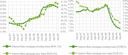
Therefore, for our data sample, we match the data sample as considered in time regimes (before and after the financial distress) with the regimes out of the credit policy. In this way, we confirm the idea highlighted in the literature: that macroeconomic conditions have significant effect on the credit risk assessment. If the interest rate at granting date is below 14% for a RON loan, or above the 8% for EUR then the Credit Policy I is mapped. Given the fact that these interest rate levels represent the level for the entire banking system we expect to correctly map a proportion of our sample. As it is presented in Table 3, the regime allocation according to the credit policy correctly maps the data split on time.

Table 3. Portfolio allocation based on interest rate regime (Source: authors’ computation).

	Regime I	Regime II	Total
Credit Policy I	4999	3424	8423
Credit Policy II	3761	5336	9097
Total	8760	8760	17,520

The sample used contains 17,520 private individuals who were active in 2006 and defaulted in 2007Q3-2008Q2 (Regime I), respectively, 2008Q3-2009Q2 (Regime II). The source of data is a private commercial bank from Romania. The data is divided equally in these two samples with 50% default rate per portfolio. The predictors are socio-demographic variables used in the application scorecard at the granting date of the loan and the financial creditworthy the debtor has, as the net income and historical delinquency behaviour as the credit bureau information.

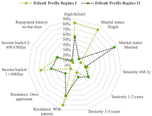
The default profile before for Regime I is a profile of a debtor with 29 average age, with high school education, having a seniority at the last job less than 2 years, living with parents, single and earning less than 400 Eur. The data on Regime II show similar core structure but with significant changes such as: only 55.14% have high school comparing with 82.24% during Regime I, only 14.63% are single while the remaining proportion of individuals are married, the seniority has increased in the second regime, the average income is 550 Eur, the average age is 35 and 23.77% have their own apartment comparing with 10.68% on Regime I (see Figure 2).

Figure 2. The default profile in Regime I and Regime II (Source: authors’ computation).

As we identify a shift in the profile of the defaulter prior and after the financial distress, we will apply the classification ensemble trees on each sample and compare the prediction accuracy by counting the misclassified cases. The shifts in the default profile shows that for a behavioural model developed on sample before the financial distress the accuracy might decrease when the profile changes. What we observed is that error Types I and II had different costs before the financial distress while after, the cost included also the opportunity costs, given the financial uncertainty. In this respect we applied different algorithms with different cost function and compare the accuracy and the total costs for each portfolio. We used the Bayesian Optimiser to search among ensemble algorithms both boosting and bagging and search among hyperparameters by giving these ranges:

• Ensemble methods: Boosting: AdaBoost, Logit Boost, Gentle Boost and Bag: Random Forest

• Maximum number of splits: [1, max (2, 8760–1)] per regime sample

• Number of learners: [10,500].

• Learning rate: [0.001,1].

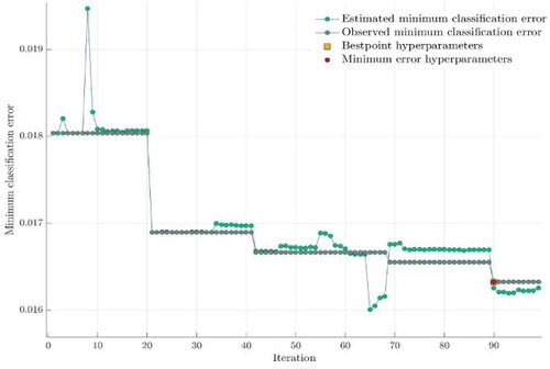
For Regime I data sample, the first step is to search among ensemble methods for the first cost function ($f_0$) without any penalty costs as the assumption is that there is no trade-off between market share and capital. We plot the minimum classification error for 100 iterations and observe that best point hyperparameters and minimum error point is for ensemble method Logit Boost with 481 number of learnings. The learning rate is 0.017377 using 30 maximum number of splits and got reached at the 90th iteration (see Figure 3).

Figure 3. Minimum classification error in Regime I (Source: authors’ computation).

The next step is to train the data on each cost functions and in order to observe the sensitivity on different cost functions we calculated the total cost per model. For every cost function we detailed below the results for the champion model, the best ensemble method based on Bayesian Optimiser. The minimum cost is reached by the random forest model with a cost function $f_4,$ where the cost of capital is four times higher than the cost of market share. For Regime I, we observe that the number of false negatives is smaller than for false positives for $f_0$ the baseline function with no penalty costs. The same trend is kept for $f_1$ and $f_4,$ the risk averse strategies while the trend is inversed for the mild risk averse functions, $f_2$ and $f_3$ (see Table 4).

Table 4. Champion model results in Regime I (Source: authors’ computation).

Cost functions	Ensemble method	Nr of learners	Max number of splits	Learning rate	TP	FN	FP	TN	Lost function
$f_0$	Logit Boost	481	30	0.01737	4330	50	93	4287	143.00
$f_1$	Random Forest	10	65		4331	49	106	4274	102.00
$f_2$	Random Forest	364	502		4285	95	65	4315	112.50
$f_3$	Gentle Boost	10	21	0.001516	4200	180	52	4328	97.00
$f_4$	Random Forest	58	110		4338	42	123	4257	72.75

A model’s performance is measured by quantifying the misclassified cases and average against all cases per class aiming to reach high sensitivity (defaulters’ classification) and high specificity (non-defaulters’ classification). Given the fact that the defaulters in Regime I are prior the financial distress we observed that comparing with Baseline, risk averse scenarios have a higher sensitivity and lower specificity while the other two scenarios recorded the inverse relationship.

For Regime I, we plotted the false positive and false negative rates and for baseline scenario the sensitivity is higher than the specificity meaning that the champion ensemble classifies more correctly the defaulters than the non-defaulters (see Figure 4).

Figure 4. Sensitivity and specificity in Regime I (Source: authors’ computation).

For risk averse scenarios, we observe that true positive rate is slightly increasing while the true negative rate decreases to the lowest value across all scenarios. For the more risk tolerant scenarios, the sensitivity decreases with almost 3% and specificity increases with almost 1%. The shift occurs in the risk tolerant scenario, as the more relaxed credit policy would decrease the power to detect the defaulters.

In order to keep the same level for detection power of bad customers, the scenarios considered are risk averse. Both Random Forest algorithms registered a lower number of false negatives than the baseline scenario. Given the fact that the cost savings had the best improvement on the Random Forest, the optimal choice during Regime I is this algorithm under severe risk averse scenario if we include the losses in decision. Therefore, during Regime I, a risk aversion scenario would lead to a decrease in non-defaulters’ detection, while a risk taker strategy would mean a significantly decrease in the true positive rate. The gap between sensitivity and specificity is at minimum on a risk tolerant scenario.

During Regime II, the champion ensemble model per each cost function reveal the fact that only gentle boost and random forest were selected among the other methods. When comparing the total cost, $f_3\mathrm{ }$ seems to be by far the champion model. During Regime II with default observations after the financial distress, the false negative cases outperform the false positive cases. The same trend is kept for all the results we obtained across all the cost functions (see Table 5).

Table 5. Champion model results in Regime II (Source: authors’ computation).

Cost functions	Ensemble method	Nr of learners	Max number of splits	Learning rate	TP	FN	FP	TN	Lost function
$f_0$	Gentle Boost	456	379	0.73486	4058	322	96	4284	418
$f_1$	Gentle Boost	78	884	0.15407	4066	314	109	4271	368.5
$f_2$	Random Forest	497	219		4005	375	63	4317	250.5
$f_3$	Random Forest	11	19		3868	512	18	4362	146
$f_4$	Random Forest	10	3741		4128	252	331	4049	334.75

For the baseline scenario, the champion model is Gentle Boost and the improvement in cost savings is null given there are no penalty costs. The minimum loss is recorded for the cost function ${\mathit{f}}_3,$ the Risk Taker strategy using Random Forest. The improvement in costs is given by the very low number of false positive cases the ensemble classified.

For Regime II, the baseline scenario indicates that the sensitivity is lower than specificity therefore Gentle Boost, the champion ensemble, correctly classifies more non-defaulters than defaulters therefore an increase in the sensitivity would balance the gap between the true rates. A decrease in true negative rate is observed for the risk averse scenarios, with a trade-off to a maximum specificity risk level. At the same time, the highest cost saving is brought by the riskier strategy as the number of false positives is the minimum leading to a high ratio of specificity. A shift in the strategy would occur in the severe risk scenario using Random Forest algorithm, that classifies correctly more default cases than non-default cases.

Therefore, during Regime II, a risk aversion scenario would lead to a decrease in non-defaulters’ detection, while a risk taker strategy would mean a significantly decrease in the true positive rate. The gap between sensitivity and specificity is at minimum on a severe risk averse scenario (see Figure 5).

Figure 5. Sensitivity and specificity in Regime II (Source: authors’ computation).

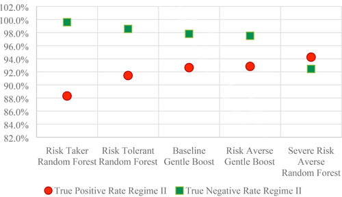
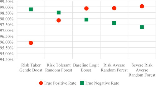
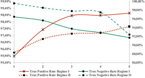
When plotting the sensitivity and specificity across regimes, we observe that for the baseline scenario, the true positive rate is above the true negative rate during the first regime and reverses on the second regime. The risk aversion leads to an improvement in default detection during both regimes and a shift in the true rates occurs during the severe risk averse scenario. The risk tolerance triggers a switch in Type I and II errors, leading to a decrease in the true positive rate. As the graph shows a risk averse scenario would bring a stable sensitivity and specificity, while a severe risk averse scenario would focus on default detection improvement. A risk tolerant policy would destabilise both default and non-default detection (see Figure 6).

Figure 6. True positive and true negative rate across scenarios for both regimes (Source: authors’ computation).

In this paper, we aim to identify the shifts in the default profile captured by a change in the regimes by using cost-sensitive ensemble methods. As Random Forest was selected for both regimes, we employed on a combined data sample the algorithm across all scenarios. We aim to observe also how maximum number of splits affect the accuracy of a classifier. The results on the aggregated portfolio (sample sized equally from the two regimes analyzed) indicate that for baseline scenario the true positive rate is lower than the true negative rate. The number of learners lies around the same value, while the maximum number of splits varies across scenarios. The minimum loss is recorded on the risk tolerant scenario as the number of false positives decreases more than the baseline scenario (see Table 6).

Table 6. Random Forest across scenarios for both regimes (Source: authors’ computation).

Cost functions	Ensemble method	Nr of learners	Max number of splits	TP	FN	FP	TN	Lost function
$f_0$	Random Forest	495	1843	3836	544	180	4200	724
$f_1$	Random Forest	486	817	3986	394	287	4093	537.5
$f_2$	Random Forest	492	2759	3753	627	103	4227	416.6
$f_3$	Random Forest	497	109	2155	2225	29	4351	585.2
$f_4$	Random Forest	476	403	4067	313	461	3919	428.25

The number of false negatives is smaller than false positives for the baseline scenario during Regime I, this means that without using any misclassification cost, the model predicts better the defaulters than non-defaulters. Given the fact that sensitivity is higher than specificity a market share strategy would mean to take more risk, as the model predicts correctly the bad customers.

During Regime I, we observed that the accuracy of the classification models increases with the risk adversity, reaching the peak on the baseline scenario. The overall accuracy for this ensemble method is 98.37% with a loss representing 1.6% from the potential total loss (is the loss that occurs when no classification model is used and is calculated assuming all cases are positive) the model could have. Ordered by accuracy the next two scenarios considered for the first regime are coming from two different strategies, capital cost and market share. Given the fact that on baseline scenario the false negative cases are smaller than false positives, the credit risk is smaller than the commercial risk. The ensemble classifies more correctly the defaulters than non-defaulters.

When we include the costs to penalise the false negative and false positive misclassification, the loss function results indicate that under risk aversion scenarios the costs are smaller comparing with the risk tolerant scenarios. During Regime I, a capital cost strategy would imply a minimum loss while a market share strategy (Risk Tolerant) would trigger a switch between the business and credit risk.

During Regime II, sensitivity is lower than specificity indicating a conservative loan policy in place as the false positive cases are lower than false negatives. The same peak in accuracy is obtained on the baseline scenario, while the minimum loss was obtained for the riskier strategies. Interesting here is to observe that during this second regime, the risk aversion increases the losses from misclassification.

During Regime II, as the false negative cases outperforms the false positive cases therefore the credit risk is higher than business risk. The baseline ensemble classifies more correctly non-defaulters than defaulters and in order to reverse it, a severe risk averse strategy should be applied.

The results on both samples combined in a portfolio presents the lower accuracy 74.27% for the most severe riskier strategy. The trend in accuracy increases with the risk aversity reaching the maximum point on the risk averse scenario. The champion model for the ensemble model under baseline scenario has the maximum misclassification cost recorded on both regimes as the average loss is lower for risk aversion scenarios than risk tolerant ones. As pointed in Figure 7 the area where both default and non-default detection would stabilise is the risk averse scenario. As we can see in Table 7, the highest accuracy for the combined regimes data was obtained on the Risk Averse scenario with 92.23% of correct classification cases where the sensitivity and specificity are high, pointed in Figure 7.

Figure 7. Sensitivity and specificity in Portfolio (Source: authors’ computation).

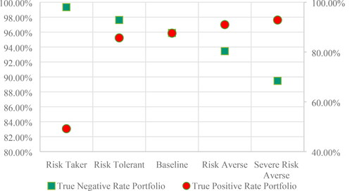
Table 7. Accuracy and loss function (Source: authors’ computation).

	Regime I	Regime II	Portfolio	Regime I	Regime II	Portfolio
Accuracy
1. Risk taker	97.35%	93.95%	74.27%	3. Baseline	3. Baseline	4. Risk averse
2. Risk tolerant	98.17%	95.00%	91.62%	4. Risk averse	4. Risk averse	3. Baseline
3. Baseline	98.37%	95.23%	91.74%	2. Risk tolerant	2. Risk tolerant	2. Risk tolerant
4. Risk averse	98.23%	95.17%	92.23%	5. Severe risk averse	1. Risk taker	5. Severe risk averse
5. Severe risk averse	98.12%	93.34%	91.16%	1. Risk taker	5. Severe risk averse	1. Risk taker
Loss function
1. Risk taker	97.0	146.0	585.2	5. Severe risk averse	1. Risk taker	2. Risk tolerant
2. Risk tolerant	112.5	250.5	416.6	1. Risk taker	2. Risk Tolerant	5. Severe risk averse
3. Baseline	143.0	418.0	724.0	4. Risk averse	5. Severe Risk Averse	4. Risk averse
4. Risk averse	102.0	368.5	537.5	2. Risk tolerant	4. Risk Averse	1. Risk taker
5. Severe risk averse	72.8	334.8	428.3	3. Baseline	3. Baseline	3. Baseline

5. Conclusions

In this paper, we aimed to identify the shifts in the default profile captured by a change in the regimes by using cost-sensitive ensemble methods. We have used four misclassification cost functions to capture the risk adversity on both samples.

The results on the Regime I show that a risk aversion scenario would lead to a decrease in non-defaulters’ detection, while a risk taker strategy would mean a significantly decrease in the true positive rate. The gap between sensitivity and specificity is at minimum on a risk tolerant scenario.

During Regime II, a risk aversion scenario would lead to a decrease in non-defaulters’ detection, while a risk taker strategy would mean a significantly decrease in the true positive rate. The gap between sensitivity and specificity is at minimum on a severe risk averse scenario. As Random Forest was selected for both regimes, we employed on a combined data sample the algorithm across all scenarios and obtained that the highest accuracy is reached when using a Random Forest Model under severe risk averse scenario.

Credit decision makers set their portfolio’s strategic benchmarks based on an objective function to meet either capital cost reduction or market share increase.

We believe the strategic decisions would benefit from being anchored to a credit policy regime and adjust it in response to shifts in economic regimes. Using cost-sensitive ensemble learning models we concluded that regime-based credit strategy can offer a better alternative in both terms of loss allocated to the strategy as well as detection power of defaulters. In this way, credit strategies are based also on the macroeconomic conditions, as highlighted in the literature (Barra & Ruggiero, 2021; Chortareas et al., 2020). Random Forest was selected for both regimes to be the best as obtained in a great number of research papers from the literature (Abellán & Castellano, 2017; Addo et al., 2018; Akindaini, 2017; Liu and Priestley 2018; Trivedi, 2020).

This paper, according to our knowledge, is the first study to explore regime-based credit strategies on a default retail loan portfolio in Romania. We consider that exploring credit strategies a priori and posteriori the financial distress (even if it is the one from 2008) is a plus for our study due to the fact that in this way our results are robust not only in good times, but also in bad times. In our opinion, this research provides an opportunity for financial institutions to build an automated model for credit risk assessment.

Some limitations of our research could be the fact that we used only one country data-Romania, so in the future we could also use data from other countries. Plus, we select four ensemble methods, and, in the future, we could expand the number of methods. A future research could imply, also, exploring the framework for credit risk strategies using data from the pandemic times. In this way, we could compare our results obtained from two crisis, with different causes.

Author contributions

This paper is the result of the joint work by all the authors. Ana-Maria Sandica elaborated the research methodology and empirical results. Alexandra Fratila (Adam) wrote the introduction and the literature review section. Both authors wrote the conclusion section. All authors have discussed and agreed to submit the manuscript.

Disclosure statement

Authors do not have any competing financial, professional or personal interests from other parties.

References

- Abellán, J., & Castellano, J. G. (2017). A comparative study on base classifiers in ensemble methods for credit scoring. Expert Systems with Applications, 73, 1–10. https://doi.org/10.1016/j.eswa.2016.12.020
- Addo, P. M., Guegan, D., & Hassani, B. (2018). Credit risk analysis using machine and deep learning models. Risks, 6(2), 38. https://doi.org/10.3390/risks6020038
- Akindaini, B. (2017). Machine learning applications in mortgage default predictions. http://tampub.uta.fi/bitstream/handle/10024/102533/1513083673.pdf
- Allen, F., Jackowicz, K., Kowalewski, O., & Kozłowski, Ł. (2017). Bank lending, crises, and changing ownership structure in Central and Eastern European countries. Journal of Corporate Finance, 42, 494–515. https://doi.org/10.1016/j.jcorpfin.2015.05.001
- Barra, C., & Ruggiero, N. (2021). Do microeconomic and macroeconomic factors influence Italian bank credit risk in different local markets? Evidence from cooperative and non-cooperative banks. Journal of Economics and Business, 114, 105976. https://doi.org/10.1016/j.jeconbus.2020.105976
- Breiman, L. (1996). Bagging predictors. Machine Learning, 24(2), 123–140. https://doi.org/10.1007/BF00058655
- Breiman, L. (2001). Random forests. Machine Learning, 45(1), 5–32. https://doi.org/10.1023/A:1010933404324
- Charpignon, M.-L., Horel, E., & Tixier, F. (2014). Prediction of consumer credit risk. CS229. http://cs229.stanford.edu/proj2014/Marie-Laure%20Charpignon,%20Enguerrand%20Horel,%20Flora%20Tixier,%20Prediction%20of%20consumer%20credit%20risk.pdf
- Chen, R., Chen, X., Jin, C., Chen, Y., & Chen, J. (2020). Credit rating of online lending borrowers using recovery rates. International Review of Economics & Finance, 68, 204–216. https://doi.org/10.1016/j.iref.2020.04.003
- Chen, T., He, J., & Li, X. (2016). An evolving network model of credit risk contagion in the financial market. Technological and Economic Development of Economy, 23(1), 22–37. https://doi.org/10.3846/20294913.2015.1095808
- Chortareas, G., Magkonis, G., & Zekente, K.-M. (2020). Credit risk and the business cycle: What do we know? International Review of Financial Analysis, 67, 101421. https://doi.org/10.1016/j.irfa.2019.101421
- Colak, M. S., & Senol, A. (2021). Banking ownership and lending dynamics: Evidence from Turkish banking sector. International Review of Economics and Finance, 72, 583–605. https://doi.org/10.1016/j.iref.2020.11.014
- Corrado, L., & Rossi, I. (2019). Anatomy of credit-less recoveries. Journal of Macroeconomics, 62, 103152. https://doi.org/10.1016/j.jmacro.2019.103152
- Dima, A. M., & Vasilache, S. (2016). Credit risk modeling for companies default prediction using neural networks. Romanian Journal of Economic Forecasting, 19(3), 127–143. http://www.ipe.ro/rjef/rjef3_16/rjef3_2016p127-143.pdf
- Friedman, J. (2001). Greedy function approximation: A gradient boosting machine. Annals of Statistics, 29(5), 1189–1232. http://www.jstor.org/stable/2699986
- Hand, D. J., & Henley, W. E. (1997). Statistical classification methods in consumer credit scoring: A review. Journal of the Royal Statistical Society: Series A (Statistics in Society), 160(3), 523–541. http://www.jstor.org/stable/2983268 https://doi.org/10.1111/j.1467-985X.1997.00078.x
- Huang, X., Liu, X., & Ren, Y. (2018). Enterprise credit risk evaluation based on neural network algorithm. Cognitive Systems Research, 52, 317–324. https://doi.org/10.1016/j.cogsys.2018.07.023
- Kjosevski, J., Petkovski, M., & Naumovska, E. (2019). Bank-specific and macroeconomic determinants of non-performing loans in the Republic of Macedonia: Comparative analysis of enterprise and households NPLs. Economic Research-Ekonomska Istraživanja, 32(1), 1185–1203. https://doi.org/10.1080/1331677X.2019.1627894
- Kruppa, J., Schwarz, A., Arminger, G., & Ziegler, A. (2013). Consumer credit risk: Individuals probability estimates using machine learning. Expert Systems with Applications, 40(13), 5125–5131. https://doi.org/10.1016/j.eswa.2013.03.019
- Ma, X., Sha, J., Wang, D., Yu, Y., Yang, Q., & Niu, X. (2018). Study on a prediction P2P network loan default based on the machine learning LightGBM and XGboost algorithms according to different high dimensional data cleaning. Electronic Commerce Research and Applications, 31, 24–39. https://doi.org/10.1016/j.elerap.2018.08.002
- Liu, L., & Priestley, J. L. (2018). A comparison of machine learning algorithms for prediction of past due service in commercial credit. Grey Literature from PhD Candidates, 8. https://digitalcommons.kennesaw.edu/dataphdgreylit/8
- Mason, L., Baxter, J., Bartlett, P., & Frean, M. (2000). Boosting algorithms as gradient descent. https://papers.nips.cc/paper/1766-boosting-algorithms-as-gradient-descent.pdf
- National Bank of Romania. (2009). Financial stability report. https://bnr.ro/Regular-publications-2504.aspx
- Ruxanda, G., Zamfir, C., & Muraru, A. (2018). Predicting financial distress for Romanian companies. Technological and Economic Development of Economy, 24(6), 2318–2337. https://doi.org/10.3846/tede.2018.6736
- Saidi, M., Daho, M., Settouti, N., & Bechar, M. (2018). Comparison of ensemble cost sensitive algorithms: Application to credit scoring prediction. http://ceur-ws.org/Vol-2326/paper7.pdf
- Schapire, R. E., & Freund, F. (2012). Boosting: Foundations and algorithms. The MIT Press.
- Siddiqi, N. (2017). Intelligent credit scoring. Building and implementing better credit risk scorecards (2nd ed.). Wiley Publishing House.
- Shen, F., Wang, R., & Shen, Y. (2019). A cost-sensitive logistic regression credit scoring model based on multi-objective optimization approach. Technological and Economic Development of Economy, 26(2), 405–429. https://doi.org/10.3846/tede.2019.11337
- Stoenescu Cimpoeru, S. (2011). Neural networks and their application in credit risk assessment. Evidence from the Romanian market. Technological and Economic Development of Economy, 17(3), 519–534. https://doi.org/10.3846/20294913.2011.606339
- Trivedi, S. K. (2020). A study on credit scoring modeling with different feature selection and machine learning approaches. Technology in Society, 63, 101413. https://doi.org/10.1016/j.techsoc.2020.101413
- Xia, Y., He, L., Li, Y., Fu, Y., & Xu, Y. (2020a). A dynamic credit scoring model based on survival gradient boosting decision tree approach. Technological and Economic Development of Economy, 27(1), 96–119. https://doi.org/10.3846/tede.2020.13997
- Xia, Y., He, L., Li, Y., Liu, N., & Ding, Y. (2020b). Predicting loan default in peer-to-peer lending using narrative data. Journal of Forecasting, 39(2), 260–280. https://doi.org/10.1002/for.2625
- Xia, Y., Liu, C., Da, B., & Xie, F. (2018a). A novel heterogeneous ensemble credit scoring model based on bstacking approach. Expert Systems with Applications, 93, 182–199. https://doi.org/10.1016/j.eswa.2017.10.022
- Xia, Y., Yang, X., & Zhang, Y. (2018b). A rejection inference technique based on contrastive pessimistic likelihood estimation for P2P lending. Electronic Commerce Research and Applications, 30, 111–124. https://doi.org/10.1016/j.elerap.2018.05.011
- Zelenkov, Y. (2019). Example-dependent cost-sensitive adaptive boosting. Expert Systems with Applications, 135, 71–82. https://doi.org/10.1016/j.eswa.2019.06.009