Research on systemic risk contagion of Chinese financial institutions based on GARCH-VMD-Copula-CoVaR model

Abstract

With the development of China's financial market, the risk contagion effect among financial institutions is increasing and becoming more complicated. Few literatures have explored the risk transmission paths of Chinese financial institutions at different frequencies. In order to make up for the gaps in this research field, variable mode decomposition (VMD) technology is introduced in this paper, combined with the Copula-GARCH model to construct the GARCH-VMD-Copula-CoVaR model, which describes the risk contagion paths of major financial institutions in the Chinese financial market at different frequencies (long-term, medium-term and short-term). The research results show that risk dependence and contagion between financial institutions have the characteristics of bidirectionality, asymmetry and time-varying in all frequency studies, and there are differences in different frequencies.

Keywords:

• Financial institutions
• risk contagion
• VMD decomposition
• Copula-CoVaR model

JEL CLASSIFICATIONS:

• E50
• E60
• G10
• G28

1. Introduction

A series of factors such as inherent emotional bias, information asymmetry and insufficient liquidity during the crisis in the financial market make it difficult to avoid risk contagion in the financial market (Calvo & Mendoza, 2000; Kyle & Wei, 2001; Xiong, 2001). The path of risk contagion between financial institutions has an important impact on financial stability. Therefore, exploring the risk contagion between financial institutions is of great significance to market investors, researchers, and policy makers (Calluzzo & Dong, 2015; Li et al., 2019; Shen & Li, 2020).

After the global financial crisis, the research on risk contagion faces two major dilemmas. First, traditional linear statistical methods are difficult to effectively capture the asymmetric dynamic changes between financial institutions. Second, the traditional analysis of risk contagion on a single frequency cannot reflect the full picture of risk contagion, and it is easy to cause overestimation or underestimation of risk (Fan & Wang, 2007).

Based on the above research background, this paper introduces advanced signal decomposition technology and combines the Copula-CoVaR model to construct the GARCH-VMD-Copula-CoVaR model to explore the risk linkage of different financial sectors in China's financial market at different frequencies. The Copula model can effectively characterize the nonlinearity and asymmetry of the asset return sequence (Berger, 2013; Embrechts & McNeil, 2002; Hsu et al., 2012), and has been widely used in financial risk research (Aloui et al., 2016; Avdulaj & Barunik, 2015; Pircalabu et al., 2017). Multi-frequency analysis based on time series can fully identify its internal characteristics at different time frequencies, and has been widely applied in various fields of research in recent years (e.g., Bouri et al., 2020; Eickmeier & Breitung, 2006; Ftiti, 2010; Jiang & Yoon, 2020; Lemmens et al., 2008; Rahim & Masih, 2016; Yang et al., 2018). Compared with other existing signal processing methods (such as wavelet transform, wavelet packet decomposition, empirical mode decomposition and integrated empirical mode decomposition), the variable mode decomposition (VMD) (Dragomiretskiy & Zosso, 2014) selected in this paper, as an improved decomposition technique, can adaptively decompose the effective components corresponding to each center frequency in the frequency domain (Jiang et al., 2017).

Our research is a supplement to the existing research literature on risk contagion of financial institutions. The rest of this paper is arranged as follows. Section 2 is a literature review. Section 3 briefly introduces the sub-models that make up the GARCH-VMD-Copula-CoVaR model and the specific steps to construct the GARCH-VMD-Copula-CoVaR model. Section 4 is an empirical analysis based on the actual data of China's financial market. Section 5 is the conclusion of this paper.

2. Literature review

A large amount of empirical literature attempts to use different econometric methods to describe the risk contagion among financial institutions. Compared with other models (e.g., the vector autoregressive model; shapley value; marginal expected loss and systemic risk index), the Conditional Value at Risk (CoVaR) model (Adrian & Brunnermeier, 2011) can effectively evaluate the risk spillover caused by a financial institution to other financial institutions after it is in trouble, and it has been widely used in the study of financial risk contagion (Choi & Shin, 2019; Nolde & Zhang, 2020; Pagano & Sedunov, 2016). Based on CoVaR method, Khiari and Ben (2019) evaluated the exposure degree and contribution of systemic risks of listed banks, so as to find the institutions that contribute the most to systemic risks. Xu et al. (2019) explored the interconnection and systemic risks of Chinese financial institutions during the period of 2010–2017 based on the LASSO-CoVaR network.

Furthermore, rich joint distributions can be constructed by introducing the combination of Copula function and marginal distribution (Huynh et al., 2020; Rivera-Castro et al., 2018; Wang et al., 2021). Reboredo and Ugolin (2015) proposed a more simplified and flexible Copula-CoVaR method and applied it to the study of systemic risks of European sovereign debt crises. Yang et al. (2019) used real volatility to measure contingent value at risk (CoVaR) and contingent expected shortage (CoES) to explore the change of risk spillover between China stock market and London stock market. Ji et al. (2020) used the time-varying Copula model based on Markov transformation and the conditional value at risk (CoVAR) to study the risk contagion between the US stock market and the rest of the G7 stock markets.

In order to distinguish the changes of financial institutions' risk contagion at different frequencies, this paper uses VMD, an advanced multi-resolution technology, to decompose the return sequence of financial institutions. In the existing research on risk contagion combined with decomposition technology. Dewandaru et al. (2016) conducted risk contagion research on major stock markets in the Asia-Pacific region based on wavelet decomposition. Shahzad et al. (2017) analyzed the risk dependence path between the US industry-level credit markets based on the copula function and VMD technology. Li and Wei (2018) investigated the correlation structure between crude oil market and Chinese stock market before and after the financial crisis by combining VMD technology with various static and time-varying copula functions. Wang et al. (2020) studied the dynamics of risk spillovers between China’s ‘black’ futures from 2013 to 2018 based on the DCC-GARCH-t model and VMD technology.

3. Methodology

This section briefly describes the marginal distribution model, VMD technology, basic Copula function, and CoVaR model that constitute the GARCH-VMD-Copula-CoVaR model, and introduces the main steps of constructing the GARCH-VMD-Copula-CoVaR model.

3.1. The marginal distribution model

Value at Risk (VaR) is defined as the maximum loss in a given time range under a given confidence level. Mathematically, set $P_t$ to be the price of financial assets on day $t,$ and VaR on the $k$ th day is defined as: (1) $$\left(P_{t-k}-P_t\le \mathit{VaR}\left(t,k,\alpha \right)\right)=1-\alpha$$(1)

Further, the 1-day logarithmic rate of return on day $t$ is defined as $r_t=\mathit{log}\left(P_t\right)-\mathit{log}\left(P_{t-1}\right).$ In this article, using VaR as the standard, four GARCH models, GARCH model, IGARCH model, EGARCH model and EGARCH model, are selected to investigate the ability of fitting the edge distribution of each yield series. The basic model of GARCH (1,1) used in this article is as follows: (2) $$r_t=c_1+{\epsilon }_{t-1}$$(2) (3) $${\sigma }_t^2=c_2+\alpha {\epsilon }_{t-1}+{\beta \sigma }_{t-1}^2$$(3)

3.2. VMD

VMD technology decomposes the input signal into a series of sparse component signals, and determines the bandwidth and center frequency of the component signal by solving the variational problem of the mode component. The main steps of VMD decomposition are as follows:

Step 1: Perform Hilbert transform on the component signal to obtain the unilateral spectrum, and further obtain the following constrained variational modal optimization problem: (4) $$\{\begin{array}{c}\underset{\left\{u_k\right\},\left\{w_k\right\}}{\mathit{min}}\left\{{\sum }_k\Vert {\partial }_t\left[\left(\delta \right(t)+\frac{j}{\pi t})\mathrm{*}{u}_k\left(t\right)\right]e^{-j{w}_{k}t}\Vert \begin{array}{c}2\\ 2\end{array}\right\}\\ s.t.{\sum }_k{u}_k=f\mathrm{ }\end{array}.$$(4)

In the formula, $\left\{u_k\right\}:=\{u_1,\dots ,u_K\},$ $\left\{w_k\right\}:=\{w_1,\dots ,w_K\}$ are the VMF of each modal component after VMD decomposition and the corresponding center frequency of each VMF. ${\partial }_t$ represents the partial derivative of $t,$ $\delta (t)$ is the impact function, $\mathrm{*}$ is the convolution symbol, and $f$ is the original input signal. Obtain the analytical signal of the relevant $u_k(t)$ through the Hilbert transform to obtain its unilateral spectrum. The exponential term $e^{-j{w}_{k}t}$ is used to adjust the estimated value of each $w_k$ and integrate the spectrum of $u_k$ into the basic frequency band.

Step 2: In order to obtain the optimal solution of the above constrained variational modes and ensure the accuracy of signal reconstruction and strict constraint conditions, the quadratic penalty function term $\alpha$ and Lagrange multiplier $\lambda$ are introduced. Therefore, the constrained variational modal calculation formula becomes the following form: (5) $$L\left(\left\{u_k\right\},\left\{w_k\right\},\lambda \right):=\alpha {{\sum }_k\Vert {\partial }_t\left[\left(\delta \right(t)+\frac{j}{\pi t})\mathrm{*}{u}_k\left(t\right)\right]e^{-j{w}_{k}t}\Vert }_2^2+{\Vert f\left(t\right)-\mathrm{ }{\sum }_k{u}_k\left(t\right)\Vert }_2^2+⟨\lambda \left(t\right),f\left(t\right)-{\sum }_k{u}_k\left(t\right)⟩$$(5)

Step 3: Through the Alternating Direction Method of Multipliers (ADMM) algorithm, the formulas (6) to (8) are repeatedly iterated to obtain ${\widehat{u}}_k^{n+1}\left(w\right),{\widehat{\mathrm{w}}}_{\mathrm{k}}^{\mathrm{n}+1},$ ${\widehat{\lambda }}^{n+1}$ to solve the above-mentioned variational problem, and stop iterating until the convergence condition (9) is satisfied to obtain the optimal solution of the constrained variational model. (6) $${\widehat{u}}_k^{n+1}\left(w\right)=\frac{\widehat{f}\left(w\right)-{\sum }_{i\ne k}\widehat{u_i}\left(w\right)+\frac{\widehat{\lambda }\left(w\right)}{2}}{1+2\alpha (w-w_k{)}^2}$$(6) (7) $${\widehat{\mathrm{w}}}_{\mathrm{k}}^{\mathrm{n}+1}=\frac{{\int }_0^{\mathrm{\infty }}\mathrm{w}{\left|{\widehat{\mathrm{u}}}_{\mathrm{k}}\left(\mathrm{w}\right)\right|}^2\mathrm{d}\mathrm{w}}{{\int }_0^{\mathrm{\infty }}{\widehat{\mathrm{u}}}_{\mathrm{k}}{\left|\left(\mathrm{w}\right)\right|}^2\mathrm{d}\mathrm{w}}$$(7) (8) $${\widehat{\lambda }}^{n+1}={\widehat{\lambda }}^n+\tau \left[\widehat{f}\right(w)-{\sum }_k{\widehat{u}}_k^{n+1}\left(w\right)]$$(8)

In the formula, ${\widehat{u}}_k^n(w),$ $\widehat{f}(w)$ and$\mathrm{ }{\widehat{\lambda }}^n(w)$ are the Fourier transforms corresponding to ${\widehat{u}}_k^n,$$\mathrm{ }f(t)$ and ${\lambda }^n,$ respectively. (9) $$\frac{{\sum }_k\parallel {\widehat{u}}_k^{n+1}-{\widehat{u}}_k^n{\parallel }_2^2}{\parallel {\widehat{u}}_k^n{\parallel }_2^2}<\epsilon$$(9)

3.3. Basic theory of Copula function

Copula theory was first proposed by Sklar. For continuous $k$-element distributions, it can be divided into Copula functions and $k$ edge distributions. According to Sklar's theorem, $X={\left(x_1,x_2,\dots x_n\right)}^T$ represents a random vector, $F\left(·,\dots ,·\right)$ represents its joint distribution function. For $i\in \left\{1,\dots ,n\right\},$$\mathrm{ }{F}_i\left(·\right)$ is the marginal distribution corresponding to $x_i,$ then there is a Copula function ${\left[0,1\right]}^N\to \left[0,1\right],$ based on the above, we can get: (10) $$F\left(x_1,x_2,\dots x_n\right)=C\left\{F_1\left(x_1\right),F_2\left(x_2\right),\dots ,F_n\left(x_n\right)\right\}$$(10)

If $F_i\left(·\right)$ represents a continuous function, then the only corresponding Copula function can be obtained at this time. If $F_i\left(·\right)$ represents a univariate distribution function, and $C\left(·,\dots ,·\right)$ represents the corresponding Copula function, then the function $F\left(·,\dots ,·\right)$ represents the joint distribution of the random variable $X.$ Therefore, let $F\left(·,\dots ,·\right)$ be the joint distribution function of the marginal distribution $F_i\left(·\right),$ $C\left(·,\dots ,·\right)$ be the corresponding Copula function, $F_i^{(-1)}\left(i=1,2,\dots N\right)$ is the pseudo-inverse function of $F_i\left(·\right),$ then any $\left(u_1,u_2,\dots u_n\right)$ in the domain of the function $C\left(·,\dots ,·\right)$ has the following form: (11) $$C\left(u_1,u_2,\dots u_n\right)={F(F}_1^{\left(-1\right)}\left(u_1\right),F_2^{\left(-1\right)}\left(u_2\right),\dots ,F_N^{\left(-1\right)}\left(u_N\right))$$(11)

In addition, the density function of the joint distribution can be obtained by the density function of the Copula function and the density function of the edge distribution: (12) $$f\left(x_1,x_2,\dots x_n\right)=C\left(F_1\left(x_1\right),F_2\left(x_2\right),\dots ,F_n\left(x_n\right)\right)\times \prod _{i=1}^n{f}_i\left(x_i\right)$$(12)

Among them, $c\left(u_1,u_2,\dots u_n\right)=\frac{{\partial }^n}{\partial u_1\cdots \partial u_n}C\left(u_1,u_2,\dots u_n\right),$$\mathrm{ }{f}_i(x_i)$ is the density function of the marginal distribution $F_i\left(x_i\right).$

3.4. CoVaR model

Adrian and Brunnermeier (2011) established CoVaR model based on VaR model and considering risk spillover effect among financial institutions. It represents the maximum loss value that other asset portfolios may produce when the loss of one asset is equal to VaR at a given probability level in a specific time. Therefore, given the confidence level of $1-q,$ when the loss value of financial institution $i$ is VaR, its expression is as follows: (13) $$P_r\left(\right(Y^j\le Va{R}_{\beta }^{j/i}\left|Y^i=Va{R}_{\alpha }^i\right))=\beta$$(13)

3.5. The GARCH-VMD-Copula-CoVaR model

Based on the sub-model introduced above, this paper constructs a new GARCH-VMD-Copula-CoVaR model to characterize the risk contagion of different financial institutions at different frequencies. Specifically, the GARCH-VMD-Copula-CoVaR model constructed in this paper mainly includes the following four main steps.

Step 1: Fitting the marginal distribution of asset return series. In this paper, considering the typical characteristics of asset return series, taking 5%VaR as the benchmark, GARCH model, IGARCH model, EGARCH model and EGARCH model are selected respectively to fit all marginal data and calculate the relevant VaR values, so as to select the appropriate GARCH fitting model.

Step 2: Frequency domain decomposition based on VMD technology. In this paper, VMD technology is applied to decompose the standardized residual sequence filtered by GARCH model into ten intrinsic mode functions VMFs and residual terms with different time spans, so as to obtain the low frequency (intermediate frequency and high frequency) modes representing the long-term (medium-term and short-term) dynamics of the original signal. These variational models will allow us to observe the hidden changes of risk contagion of financial institutions in different periods.

Step 3: Selection of Copula function. Based on the Gsussian Copula, Student t Copula (t-Copula), Clayton Copula, Gumbel Copula, Frank Copula and Joe Copula functions, this paper estimates the risk dependence structure among financial institutions in different periods, and selects the best Copula function based on AIC function adjusted by small sample deviation.

Step 4: Risk estimation of dynamic CoVaR model. In order to explore the dynamic changes of risk spillover effects of financial institutions in different periods, this paper introduces a rolling window to build a dynamic CoVaR model to study the dynamic changes of systemic risk spillover among financial institutions in the long-term, medium-term and short-term.

4. Empirical results

4.1. Data selection and basic analysis

In this paper, the daily closing prices of bank index, securities index, fund index and insurance index are selected as sample data, and the data comes from Wind database. The sample period is from January 10, 2007 to August 24, 2020, with a total of 3301 selected samples. The sample interval covers the financial crisis in 2008, the European debt crisis in 2011, the stock market crash in China in 2015, the debt disaster in China in 2016 and the outbreak of COVID-19 in China in 2020. 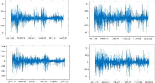Let $p_{it}$ be the daily closing price of index $i,$ and define the daily logarithmic rate of return as $r_{it}={\mathit{lnp}}_{it}$-${\mathit{lnp}}_{i,t-1}.$ The program in this article is implemented by EViews10, matlab2019a and RStudio. The trend of log returns of different samples is shown in Figure 1.

Figure 1. The trend chart of the full-sample logarithmic return rate of bank index, securities index, fund index and insurance index. The upper left corner, upper right corner, lower left corner and lower right corner are the corresponding bank index, securities index, fund index and insurance index, respectively.

Source: Authors.

Table 1 shows the results of descriptive statistical analysis on the index return sequence of various financial institutions. It can be seen that each return rate series shows a significant negative bias and peak shape. The results of the Jarque-Bera (JB) test show that the null hypothesis that the standard residuals are normally distributed at the 1% significance level is rejected, and the Augmented Dickey–Fuller (ADF) test shows that the index rejects the null hypothesis that there is a unit root at the 1% significance level, that is, the sequence is stable. In addition, EViews can provide more intuitive results for the analysis of time series. Figure 2 provides the test results of autocorrelation and partial autocorrelation of each yield series based on EViews10. The results show that the yield series of each financial institution has autocorrelation.

Figure 2. Autocorrelation and partial autocorrelation analysis chart of the return series of bank index, securities index, fund index and insurance index. The upper left corner, upper right corner, lower left corner and lower right corner are the corresponding bank index, securities index, fund index and insurance index, respectively.

Source: Authors.

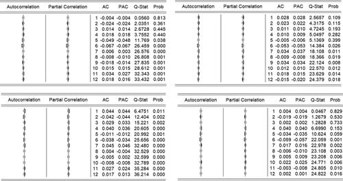
Table 1. Descriptive statistical analysis of the series of returns of financial institutions.

	Mean value	Standard deviation	Skewness	Kurtosis	The value of JB	The value of ADF
Bank index	2.65E − 04	0.019207	−0.011224	7.430418	2700.638	−57.66772
Securities index	2.30E − 04	0.027461	−0.053323	5.565394	907.0345	−55.86232
Fund index	3.46E − 04	0.010473	−0.580133	6.756238	2126.425	−54.89872
Insurance index	2.91E − 04	0.023198	−0.007128	5.726170	1022.547	−57.21422

Note. The critical value of the JB statistic at the 1% level is 9.9, and the critical value of the ADF statistic at the 1% level is −2.565663.

Source: Authors.

Furthermore, the ARCH-LM test is performed on each sequence. Table 2 contains three F statistic values of different orders, and the corresponding p value indicates that the sequence rejects the original hypothesis at a significant level of 1%. The result shows each index series has an ARCH effect, which verifies the rationality of the GARCH model used in this article.

Table 2. ARCH-LM test of index yield series of each financial institutions.

	ARCH statistics (1st order)	ARCH statistics (5th order)	ARCH statistics (10th order)
Bank index	126.6588	70.33151	45.43452
	（0.000）	（0.000）	（0.000）
Securities index	141.7654	68.62545	45.76422
	（0.000）	（0.000）	（0.000）
Fund index	125.6939	74.25905	44.95835
	（0.000）	（0.000）	（0.000）
Insurance index	77.95918	50.15402	31.80882
	（0.000）	（0.000）	（0.000）

Note. The ARCH statistic in the table is the F statistic, and the p-value of the F statistic is in parentheses.

Source: Authors.

4.2. The fitting result of the marginal distribution of the asset return series

Based on 5%VaR, GARCH fitting is carried out on all marginal data, and relevant VaR values are calculated, in which the number of prediction periods outside the sample is 2760. This paper compares the performance of four GARCH models in estimating the index of financial institutions. Table 3 shows the fitting values of GRACH models for different financial institution indexes, and Figure 3 shows the fitting results of GARCH models based on 5%VaR for different financial institution indexes.

Figure 3. Autocorrelation and partial autocorrelation analysis chart of yield series of bank index, securities index, fund index and insurance index. The upper left corner, upper right corner, lower left corner and lower right corner are the corresponding bank index, securities index, fund index and insurance index, respectively.

Source: Authors.

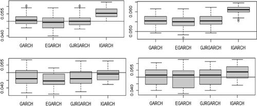
Table 3. The fitting value of GRACH models for the yield of different financial institution indexes.

	GARCH	EGARCH	GJRGARCH	IGARCH
Bank index	0.001291314	−0.000637971	0.000668716	0.005818601
Securities index	0.005488086	0.004857802	0.005588009	0.010868560
Fund index	−0.002820907	−0.004673328	−0.003420446	−0.000845504
Insurance index	0.000253846	−0.000946154	0.000284615	0.003330769

Note. The bold value represents the smallest absolute value obtained in the four GARCH models.

Source: Authors.

The results obtained show that bank index, securities index, fund index and insurance index perform best in the fitting results of EGARCH model, EGARCH model, IGARCH model and GARCH model, respectively. Therefore, the EGARCH model, the EGARCH model, the IGARCH model and the GARCH model are selected to carry out the following empirical analysis on the bank index, the securities index, the fund index and the insurance index respectively.

Further, based on the selected GARCH models of different index sequences, this paper selects Ljung-Box to test the residual sequences obtained by fitting the selected GARCH models for each index. Table 4 shows the results of Ljung-Box (5), Ljung-Box (10) and Ljung-Box (15) tests for each index residual sequence. The results show that the residual sequence of each index fitted by GARCH model obeys normal distribution, which indicates the rationality of the fitting process.

Table 4. The test results of the residual series of each index.

	Bank index (EGARCH)	Securities index (EGARCH)	Fund index (IGARCH)	Insurance index (GARCH)
Ljung-Box (5)	3.0811	3.9235	7.2392	9.4635
Ljung-Box (10)	1.2449	2.2554	2.9059	7.0739
Ljung-Box (15)	9.4118	5.3134	4.3976	2.2930

Note. The different GARCH models in brackets are the results of the selection based on 5%VaR in Table 3.

Source: Authors.

4.3. The frequency domain decomposition results based on VMD technology

In this paper, VMD technology is applied to decompose the standardized residual sequence obtained by GARCH model into ten intrinsic mode functions VMFs and the residual term with different time spans. These ten decomposition sequences are compressed around ten different corresponding center frequencies. The decomposed sequences are marked as VMD1 to VMD10 according to the order of center frequency from small to large, and the decomposed sequence with the highest center frequency (VMD10) is selected as short-term sequence, the decomposed sequence with medium center frequency (VMD5) as medium-term sequence, and the decomposed sequence with the lowest frequency (VMD1) as long-term sequence (Li & Wei, 2018).

Based on VMD decomposition technology, the components with different frequencies obtained from time series can be further combined with Copula-CoVaR function to explore the performance of risk spillovers between financial institutions at different frequencies. As an advanced decomposition technology, VMD decomposition can effectively analyze the structural attributes of data and distinguish the dynamic changes in the long-term, medium-term and short-term of the yield series. Figures 4–7, respectively show the original fluctuations of bank, securities, insurance, and fund index returns and the short-term (VMD10), medium-term (VMD5) and long-term (VMD1) sequences obtained by decomposition. As can be seen from the figure, the long-term (VMD1) sequence of each index shows a smoother dynamic pattern and the significance of volatility clustering is lower than that of the short-term (VMD10) and medium-term (VMD5) sequences.

Figure 4. VMD decomposition results of the bank index yield. The upper left corner, upper right corner, lower left corner and lower right corner are corresponding original wave sequence, VMD1, VMD5 and VMD10, respectively.

Source: Authors.

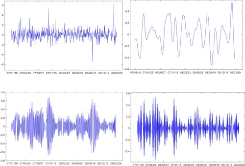
Figure 5. VMD decomposition results of the securities index yield. The upper left corner, upper right corner, lower left corner and lower right corner are corresponding original wave sequence, VMD1, VMD5 and VMD10, respectively.

Source: Authors.

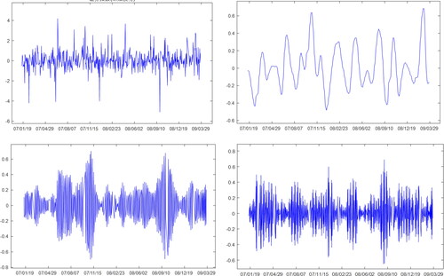
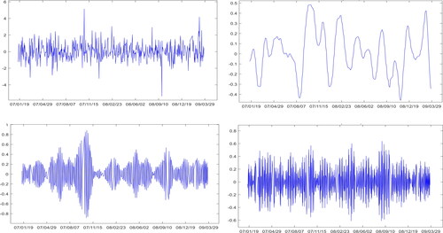
Figure 6. VMD decomposition results of the fund index yield. The upper left corner, upper right corner, lower left corner and lower right corner are corresponding original wave sequence, VMD1, VMD5 and VMD10, respectively.

Source: Authors.

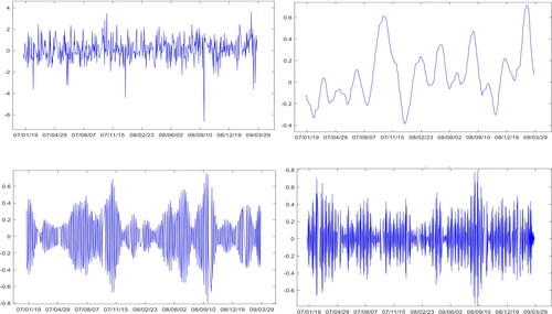
Figure 7. VMD decomposition results of the insurance index yield. The upper left corner, upper right corner, lower left corner and lower right corner are corresponding original wave sequence, VMD1, VMD5 and VMD10, respectively.

Source: Authors.

4.4. The selection result of the Copula function

After obtaining the decomposition sequence of each yield sequence in different periods, this paper uses the functions of Gaussian Copula, Student t Copula (t-Copula), Clayton Copula, Gumbel Copula, Frank Copula and Joe Copula to estimate the correlation structure between different financial institutions in different periods, and uses the AIC function adjusted for small sample deviation to select the best Copula function. Table 5 shows the specific AIC values estimated by the pairwise sequence. In general, by comparing the AIC value of each Copula function, it can be seen that the Gaussian Copula and Student t Copula (t-Copula) functions are more suitable as the estimating function of the risk contagion of financial institutions.

Table 5. Copula selection results at different frequencies.

Object	Gaussian Copula	Student t Copula (t-Copula)	Clayton Copula	Gumbel Copula	Frank Copula	Joe Copula
jjo-zqo	−579.1104	−591.8964	−509.3023	−591.4421	−533.0639	−501.5570
jjl-zql	−473.6769	−486.9346	−428.4295	−476.7239	−365.7202	−418.2706
jjm-zqm	−735.9874	−732.6760	−582.6733	−691.2241	−627.6446	−570.1931
jjs-zqs	−912.8991	−918.3786	−715.8546	−866.2430	−869.4179	−709.1918
yho-zqo	−333.8054	−352.3036	−275.5748	−335.8542	−308.9246	−266.9971
yhl-zql	−397.5808	−400.0618	−327.0322	−380.2202	−321.6456	−315.2860
yhm-zqm	−180.1053	−239.9781	−163.3024	−196.9884	−126.4636	−164.4588
yhs-zqs	−97.92486	−92.49724	−68.48438	−76.79330	−88.81014	−54.64220
bxo-zqo	−350.8493	−365.8617	−294.1351	−349.5815	−312.5815	−282.2779
bxl-zql	−342.6366	−338.3202	−282.0859	−322.4527	−327.0268	−264.9856
bxm-zqm	−432.0393	−436.2750	−332.2963	−403.0470	−386.5677	−316.4360
bxs-zqs	−524.7078	−521.7023	−402.2999	−483.8676	−492.0226	−388.5259
jjo-yho	−338.8985	−343.8324	−291.1527	−338.2955	−294.0018	−282.0677
jjl-yhl	−241.3407	−245.7508	−251.7558	−265.8425	−180.4554	−248.5998
jjm-yhm	−115.58324	−123.82607	−96.29558	−113.82953	−76.12112	−91.88392
jjs-yhs	−115.62866	−111.71587	−84.26242	−97.07639	−109.84233	−70.96836
bxo-jjo	−432.6583	−436.0428	−372.0670	−428.0665	−372.4260	−360.5390
bxl-jjl	−378.8657	−372.7087	−348.9137	−371.5141	−323.0504	−333.2395
bxm-jjm	−402.4461	−417.1893	−305.1014	−379.6357	−409.5499	−290.8674
bxs-jjs	−595.4081	−593.2000	−454.5063	−552.5247	−576.9170	−443.6676
bxo-yho	−710.0452	−714.6078	−597.6077	−698.6965	−639.6085	−589.9511
bxl-yhl	−656.6209	−646.5427	−462.5081	−568.7236	−594.6595	−446.6204
bxm-yhm	−195.0759	−199.6264	−158.8839	−188.2974	−147.5005	−150.7799
bxs-yhs	−86.02150	−80.92064	−61.73399	−67.24826	−72.69869	−48.59754

Notes. ‘yh’ stands for banks, ‘jj’ stands for funds, ‘zq’ stands for securities, ‘bx’ stands for insurance, ‘o’ stands for original, ‘m’ stands for long-term, ‘l’ stands for long-term, and ‘s’ stands for short-term. For example, ‘jjo-zqo’ represents the original risk contagion of fund index and securities index, ‘jjl-zql’ represents the long-term risk contagion of fund index and securities index, and so on.

Source: Authors.

4.5. The risk estimation results of the dynamic CoVaR model at different frequencies

In order to study the dynamic changes of risk spillover effects between banks, securities, insurance and funds in different periods, this paper introduces a rolling window to construct a dynamic CoVaR model. Define the size of the scroll window as 541, and the scroll step length as 1. Figures 8–10 show the dynamic changes in the value of systemic risk spillovers between different financial institutions in the long-term, medium-term, and short-term.

Figure 8. The long-term risk spillover effect between financial institutions under the dynamic CoVaR model. ‘yh’ stands for bank, ‘jj’ stands for fund, ‘zq’ stands for securities, ‘bx’ stands for insurance, and ‘l’ stands for long-term. For example, ‘jjl-zql’ stands for long-term risk contagion between fund index and securities index, and so on.

Source: Authors.

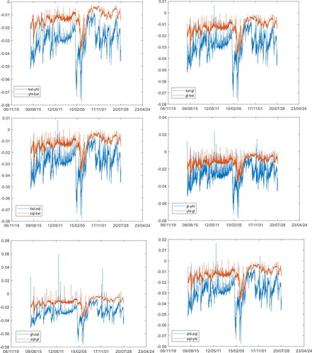
Figure 9. The medium-term risk spillover effect between financial institutions under the dynamic CoVaR model. ‘yh’ stands for bank, ‘jj’ stands for fund, ‘zq’ stands for securities, ‘bx’ stands for insurance, and ‘m’ stands for medium-term. For example, ‘jjm-zqm’ stands for medium-term risk contagion between fund index and securities index, and so on.

Source: Authors.

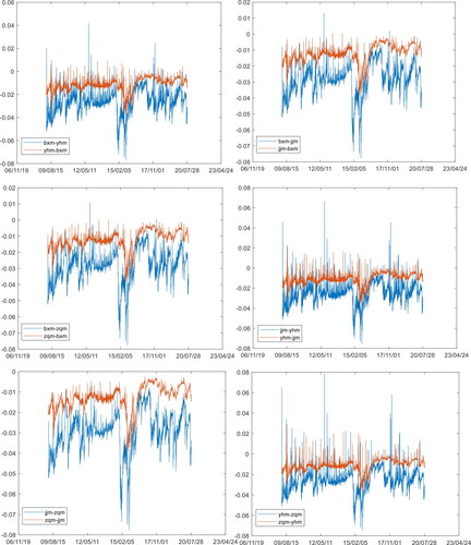
Figure 10. The short-term risk spillover effect between financial institutions under the dynamic CoVaR model. ‘yh’ stands for bank, ‘jj’ stands for fund, ‘zq’ stands for securities, ‘bx’ stands for insurance, and ‘s’ stands for short-term. For example, ‘jjs-zqs’ stands for short-term risk contagion between fund index and securities index, and so on.

Source: Authors.

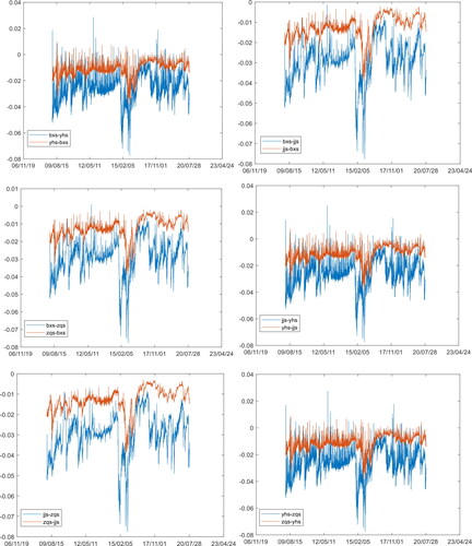
It can be seen from the figure that the volatility and intensity of risk spillover levels between various financial institutions in different periods have certain differences, but the overall trend of risk spillovers is roughly the same. The analysis in this part of this paper includes the analysis based on the overall trend in the horizontal dimension and the different frequencies in the vertical dimension. That is, based on the major events in China's financial market, the risk spillover changes of the overall trend of various financial institutions are analyzed first, and then the differences of risk spillovers in different periods are analyzed in combination with the actual business cooperation situation of financial institutions, so as to further explore the risk contagion path of financial institutions.

4.5.1. Overall trend analysis based on horizontal dimension

During the period from February 2009 to November 2010, with a series of economic stimulus plans and financial stability measures issued by the Chinese government, the systemic risk spillover level of financial institutions gradually declined as a whole. However, due to the impact of the European sovereign debt crisis, the risk spillover level increased in a local shock. Among them, at the end of August, 2010, the risk spillover value of banks, securities and funds to the insurance industry dropped significantly, which was mainly influenced by the Measures for Information Disclosure of Insurance Companies issued by China Insurance Regulatory Commission on August 5 and officially implemented on August 31 of that year. Due to the comprehensive regulation of the information disclosure of the insurance industry and the activation of corresponding restraint mechanisms on the investment of insurance funds in equity and real estate, the investment channels and business relationships of insurance funds have undergone major adjustments.

From December 2010 to November 2014, China's stock market was relatively stable, and the risk spillover level among financial institutions was generally at a controllable level. Influenced by regulatory policies and investor sentiment, the risk spillover level among different financial institutions showed differences. From September 2011 to June 2012, the level of risk spillover from banks, securities, and funds to the insurance industry increased, mainly because the new chairman of the Insurance Regulatory Commission took office and led a series of new market-oriented insurance reform policies, which triggered huge fluctuations in the capital market. From October 2012 to August 2013, the level of risk spillovers from banks, insurance, and funds to the securities industry increased volatically. During the period from March 2013 to August 2014, the risk spillover level of securities, insurance and funds to the banking industry showed a turbulent rise, which was not only impacted by the shortage of market funds to the stock market, but also influenced by market supervision policies and investor sentiment.

During the period from November 2014 to August 2017, China's stock market first experienced a rapid and violent decline after the reform, followed by a period of stable operation (March 2016–August 2017). From August 2017 to August 2020, the risk spillover of China's stock market is still at a volatile level. During the outbreak of COVID-19 epidemic in early 2020, the level of risk spillover in China's stock market increased significantly, indicating the impact of major social events on the development of the stock market. When the confidence and prospect of social and economic development are shaken, the financial market will also reflect the risks brought by this uncertain expectation.

Compared with the results of the traditional research path followed in this paper, the results of this paper in the horizontal dimension are consistent with them. The overall evolution of risk spillovers is in line with the actual trend of China's stock market during the sample period, which indicates the rationality of the model construction in this paper. In addition, the research results of this paper show that the characteristics of systemic risk spillovers of China’s financial institutions in the horizontal dimension are bidirectional, asymmetry, and time-varying. Among them, during the periods of European sovereign debt crisis and the stock market crash, the intensity of systemic risk spillovers among financial institutions was higher than in other periods of the sample period.

4.5.2. The analysis of different frequencies based on the longitudinal dimension

In the actual business relationship of China's financial market, the business of financial institutions is relatively homogeneous. Therefore, the ability of financial institutions to actively manage funds has become their core competitiveness in the financial market. The fund management in financial market can be roughly divided into three parts, namely, the source of funds, the investment management of funds and the channel connecting institutions between them. In China, the source institution of funds is mainly represented by banks, whose main function is to absorb funds; the investment management institution of funds is mainly represented by funds, which obtain income through the operation of funds; channel institutions are mainly represented by securities, which mainly provide convenient trading services.

It can be seen from the result graph that there are differences and asymmetries in risk spillovers at different frequencies among financial institutions. In the differential performance of risk spillovers, the fund industry and the insurance industry have the largest risk spillover value to the securities industry; the banking and securities industry has the second highest risk spillover value to the insurance industry; and the banking, insurance and securities industries have the minimal risk spillover effect on the fund industry. In addition, in the asymmetric performance of risk spillovers, the level of risk spillover from the banking industry to the insurance industry is greater than that of the insurance industry; the level of risk spillover from the securities industry to the banking industry and the insurance industry is greater than that of these two sub-markets; and the risk spillover level of the fund industry to the banking, insurance and securities industries is greater than the spillover level of these three sub-markets. Further, the specific analysis of risk spillovers at different frequencies between financial institutions is as follows: In the analysis of different periods of risk contagion in the banking and securities industries, the risk spillover effect is stronger in the long term, and the volatility of the risk spillover is greater in the short term. This phenomenon arises from the close cooperation between banks and securities in the long term. The content of their business cooperation includes fund custody, clearing, payment and other businesses. The capital source of the securities industry mainly relies on market financing. If the securities industry encounters a risk event, the risk will affect the banking industry through the asset-liability channel; in the short term, once a systemic risk event occurs in the banking industry, the risk will be transmitted to the securities industry through investor sentiment and other channels.

In the research on risk spillovers from the banking and securities industries to the insurance industry, the intensity of the risk spillovers from the securities industry to the insurance industry is roughly the same in different frequencies. Compared with the medium-term and long-term, the risk spillover of the banking industry to the insurance industry shows strong volatility in the short-term, indicating the close linkage between the banking industry and the insurance industry in the short-term risk spillover. This phenomenon stems from the single mode of cooperation between the securities industry and the insurance industry, in which the insurance industry provides financing needs for the securities industry, and the securities industry acts as an agent for the insurance industry to buy and sell securities. In contrast, the cooperation mode between banks and insurance is relatively close. Because banks sell insurance products as agents in practice and the existence of deposit insurance system, when banks take risks, they will cause panic in the market and affect the insurance industry through investor sentiment and balance sheet channels.

In the research on the risk spillovers of banking, insurance and securities industries to the fund industry, the medium- and long-term risk spillovers are relatively high, while the short-term risk spillovers of the fund industry and the securities industry have the lowest volatility, and the volatility of the risk spillovers between banking and fund industry is the highest. This phenomenon stems from the fact that fund management companies are China’s earliest legally principal asset management financial institutions, and its business relationship with the banking industry is close. The main business of the fund management company includes public fund raising business and asset management business for specific customers.

Based on the above analysis, it can be concluded that risk spillovers at different frequencies all have the characteristics of bidirectionality, asymmetry, and time-varying. Systemic risk spillovers among China’s financial institutions are affected by factors such as government regulatory policies and investor sentiment. Due to the differences in the business characteristics of institutions, the intensity of risk spillovers between financial institutions differs at different frequencies. The risk spillover performance of financial institutions in long-term and medium-term frequency is mainly affected by the financial institutions' ability to actively manage funds. In addition, in the performance of the intensity of risk spillovers, the intensity of the long-term, medium-term and short-term frequency show a decreasing trend. In the volatility performance of risk spillovers, the volatility of long-term, medium-term and short-term frequency show an increasing trend.

5. Conclusions

Although there is a large amount of empirical literature on risk contagion of financial institutions, few studies have explored the evolutionary path of risk spillovers between financial institutions at different frequencies. This paper first fits the marginal distribution of the return rate series of various financial institutions with GARCH models, then a series of copula functions are combined with the VMD decomposition technique, and the GARCH-VMD-Copula-CoVaR model is further constructed by combining with the dynamic CoVaR model, which measures the risk transmission paths among the four financial sectors of banking, insurance, fund and securities in different frequencies in China's financial market.

The main conclusions of this paper are as follows: (1) the overall evolution trend of risk spillover among financial institutions obtained by GARCH-VMD-Copula-CoVaR model constructed in this paper accords with the actual trend of China's stock market during the sample period; (2) risk spillovers at different frequencies are all bidirectional, asymmetry and time-varying, the intensity of risk spillovers is stronger in the long-term frequency, and the volatility of risk spillovers is greater in the short-term frequency; (3) the level of risk spillover among financial institutions at different frequencies is influenced by China's major regulatory policies and business cooperation modes among banking, insurance, securities and fund industries.

Considering the economic impact of the world economy on China's financial market and the volatility of risk spillovers among financial institutions in the financial market, our research results can help researchers understand the application of decomposition technology in financial time series and risk contagion to a certain extent; it is beneficial for the risk managers to improve the regulatory policies and avoid the economic crisis by considering the impact of the policies in different periods; and by considering the intensity and volatility characteristics of risk spillovers between financial institutions at different frequencies, it can provide useful information on the distribution weights of various assets for individual investors when formulating investment portfolios with different maturities.

Disclosure statement

The authors declare that they have no conflict of interest.

Additional information

Funding

This study was funded by two National Natural Science Foundations of China (Grant Nos. 71573042 and 71973028).

References

- Adrian, T., & Brunnermeier, M. K. (2011). CoVaR. NBER working paper. National Bureau of Economic Research.
- Aloui, R., Gupta, R., & Miller, S. M. (2016). Uncertainty and crude oil returns. Energy Economics, 55, 92–100. https://doi.org/10.1016/j.eneco.2016.01.012
- Avdulaj, K., & Barunik, J. (2015). Are benefits from oil–stocks diversification gone? New evidence from a dynamic copula and high frequency data. Energy Economics, 51, 31–44. https://doi.org/10.1016/j.eneco.2015.05.018
- Berger, T. (2013). Forecasting value-at-risk using time varying copulas and EVT return distributions. International Economics, 133, 93–106. https://doi.org/10.1016/j.inteco.2013.04.002
- Bouri, E., Shahzad, S. J. H., Roubaud, D., Kristoufek, L., & Lucey, B. (2020). Bitcoin, gold, and commodities as safe havens for stocks: New insight through wavelet analysis. The Quarterly Review of Economics and Finance, 77, 156–164. https://doi.org/10.1016/j.qref.2020.03.004
- Calluzzo, P., & Dong, G. N. (2015). Has the financial system become safer after the crisis? The changing nature of financial institution risk. Journal of Banking & Finance, 53, 233–248. https://doi.org/10.1016/j.jbankfin.2014.10.009
- Calvo, G. A., & Mendoza, E. G. (2000). Rational contagion and the globalization of securities markets. Journal of International Economics, 51(1), 79–113. https://doi.org/10.1016/S0022-1996(99)00038-0
- Choi, J. E., & Shin, D. W. (2019). Three regime bivariate normal distribution: A new estimation method for co-value-at-risk, CoVaR. The European Journal of Finance, 25(18), 1817–1833. https://doi.org/10.1080/1351847X.2019.1639208
- Dewandaru, G., Masih, R., & Masih, A. M. M. (2016). Contagion and interdependence across Asia-Pacific equity markets: An analysis based on multi-horizon discrete and continuous wavelet transformations. International Review of Economics & Finance, 43, 363–377. https://doi.org/10.1016/j.iref.2016.01.002
- Dragomiretskiy, K., & Zosso, D. (2014). Variational mode decomposition. IEEE Transactions on Signal Processing, 62(3), 531–544. https://doi.org/10.1109/TSP.2013.2288675
- Eickmeier, S., & Breitung, J. (2006). How synchronized are new EU member states with the euro area? Evidence from a structural factor model. Journal of Comparative Economics, 34(3), 538–563. https://doi.org/10.1016/j.jce.2006.06.003
- Embrechts, P. A., & McNeil, D. S. (2002). Correlation and dependence in risk management: Properties and pitfalls. In Risk management: Value at risk and beyond (pp. 176–223). Cambridge University Press.
- Fan, J., & Wang, Y. (2007). Multi-scale jump and volatility analysis for high-frequency financial data. Journal of the American Statistical Association, 102(480), 1349–1362. https://doi.org/10.1198/016214507000001067
- Ftiti, Z. (2010). The macroeconomic performance of the inflation targeting policy: An approach based on the evolutionary co-spectral analysis (extension for the case of a multivariate process). Economic Modelling, 27(1), 468–476. https://doi.org/10.1016/j.econmod.2009.10.013
- Hsu, C. P., Huang, C. W., & Chiou, W. J. P. (2012). Effectiveness of copula-extreme value theory in estimating value-at-risk: Empirical evidence from Asian emerging markets. Review of Quantitative Finance and Accounting, 39(4), 447–468. https://doi.org/10.1007/s11156-011-0261-0
- Huynh, T. L. D., Nasir, M. A., Nguyen, S. P., & Duong, D. (2020). An assessment of contagion risks in the banking system using non-parametric and Copula approaches. Economic Analysis and Policy, 65, 105–116. https://doi.org/10.1016/j.eap.2019.11.007
- Ji, Q., Liu, B.-Y., Cunado, J., & Gupta, R. (2020). Risk spillover between the US and the remaining G7 stock markets using time-varying copulas with Markov switching: Evidence from over a century of data. The North American Journal of Economics and Finance, 51, 100846. https://doi.org/10.1016/j.najef.2018.09.004
- Jiang, Y., Nie, H., & Monginsidi, J. Y. (2017). Co-movement of ASEAN stock markets: New evidence from wavelet and VMD-based copula tests. Economic Modelling, 64, 384–398. https://doi.org/10.1016/j.econmod.2017.04.012
- Jiang, Z. H., & Yoon, S. M. (2020). Dynamic co-movement between oil and stock markets in oil-importing and oil-exporting countries: Two types of wavelet analysis. Energy Economics, 90, 104835. https://doi.org/10.1016/j.eneco.2020.104835
- Khiari, W., & Ben, S. S. (2019). On identifying the systemically important Tunisian banks: An empirical approach based on the △CoVaR measures. Risks, 7(4), 122. https://doi.org/10.3390/risks7040122
- Kyle, A. S., & Wei, X. (2001). Contagion as a wealth effect. The Journal of Finance, 56(4), 1401–1440. https://doi.org/10.1111/0022-1082.00373
- Lemmens, A., Croux, C., & Dekimpe, M. G. (2008). Measuring and testing Granger-causality over the spectrum: An application to European production expectation surveys. International Journal of Forecasting, 24(3), 414–431. https://doi.org/10.1016/j.ijforecast.2008.03.004
- Li, X., & Wei, Y. (2018). The dependence and risk spillover between crude oil market and China stock market: New evidence from a variational mode decomposition-based copula method. Energy Economics, 74, 565–581. https://doi.org/10.1016/j.eneco.2018.07.011
- Li, J., Yao, Y., Li, J., & Zhu, X. (2019). Network-based estimation of systematic and idiosyncratic contagion: The case of Chinese financial institutions. Emerging Markets Review, 40, 100624. https://doi.org/10.1016/j.ememar.2019.100624
- Nolde, N., & Zhang, J. Y. (2020). Conditional extremes in asymmetric financial markets. Journal of Business & Economic Statistics, 38(1), 201–213. https://doi.org/10.1080/07350015.2018.1476248
- Pagano, M. S., & Sedunov, J. (2016). A comprehensive approach to measuring the relation between systemic risk exposure and sovereign debt. Journal of Financial Stability, 23, 62–78. https://doi.org/10.1016/j.jfs.2016.02.001
- Pircalabu, A., Hvolby, T., Jung, J., & Høg, E. (2017). Joint price and volumetric risk in wind power trading: A copula approach. Energy Economics, 62, 139–154. https://doi.org/10.1016/j.eneco.2016.11.023
- Rahim, A. M., & Masih, M. (2016). Portfolio diversification benefits of Islamic investors with their major trading partners: Evidence from Malaysia based on MGARCH-DCC and wavelet approaches. Economic Modelling, 54, 425–438. https://doi.org/10.1016/j.econmod.2015.12.033
- Reboredo, J. C., & Ugolin, A. (2015). Systemic risk in European sovereign debt markets: A CoVaR-Copula approach. Journal of International Money and Finance, 1(C), 214–224.
- Rivera-Castro, M. A., Ugolini, A., & Zambrano, J. A. (2018). Tail systemic risk and contagion: Evidence from the Brazilian and Latin America banking network. Emerging Markets Review, 35, 164–189. https://doi.org/10.1016/j.ememar.2018.02.004
- Shahzad, S. J. H., Nor, S. M., Kumar, R. R., & Mensi, W. (2017). Interdependence and contagion among industry-level US credit markets: An application of wavelet and VMD based Copula approaches. Physica A: Statistical Mechanics and Its Applications, 466, 310–324. https://doi.org/10.1016/j.physa.2016.09.008
- Shen, P. L., & Li, Z. N. (2020). Financial contagion in inter-bank networks with overlapping portfolios. Journal of Economic Interaction and Coordination, 15(4), 845–865. https://doi.org/10.1007/s11403-019-00274-1
- Wang, Q. W., Dai, X. Y., & Zhou, D. Q. (2020). Dynamic correlation and risk contagion between ‘Black’ futures in China: A multi-scale variational mode decomposition approach. Computational Economics, 55(4), 1117–1150. https://doi.org/10.1007/s10614-018-9857-y
- Wang, H., Yuan, Y., Li, Y., & Wang, X. (2021). Financial contagion and contagion channels in the forex market: A new approach via the dynamic mixture Copula-extreme value theory. Economic Modelling, 94, 401–414. https://doi.org/10.1016/j.econmod.2020.10.002
- Xiong, W. (2001). Convergence trading with wealth effects: An amplification mechanism in financial markets. Journal of Financial Economics, 62(2), 247–292. https://doi.org/10.1016/S0304-405X(01)00078-2
- Xu, Q., Li, M., Jiang, C., & He, Y. (2019). Interconnectedness and systemic risk network of Chinese financial institutions: A LASSO-CoVaR approach. Physica A: Statistical Mechanics and Its Applications, 534, 122173. https://doi.org/10.1016/j.physa.2019.122173
- Yang, K., Wei, Y., He, J., & Li, S. (2019). Dependence and risk spillovers between mainland China and London stock markets before and after the Stock Connect programs. Physica A: Statistical Mechanics and Its Applications, 526, 120883. https://doi.org/10.1016/j.physa.2019.04.119
- Yang, L., Yang, L., & Hamori, S. (2018). Determinants of dependence structures of sovereign credit default swap spreads between G7 and BRICS countries. International Review of Financial Analysis, 59, 19–34. https://doi.org/10.1016/j.irfa.2018.06.001