Agent-based artificial financial market with evolutionary algorithm

Abstract

In traditional financial studies, existing approaches are unable to address increasingly complex problems. In this paper, an artificial financial market is proposed, in accordance with the adaptation market hypothesis, using artificial intelligence algorithms. This market includes three types of agents with different investments and risk preferences, representing the heterogeneity of traders. Genetic network programming is combined with a state-action-reward-state-action (SARSA)(λ) algorithm for designing the market to reflect the adaptation of technical agents. A pricing mechanism is taken into consideration, based on the auction mechanism of the Chinese securities market. The characteristics of price time series are analyzed to determine whether excessive volatility exists in four different markets. Explanations are provided for the corresponding financial phenomena considering the hypotheses under the proposed novel artificial financial market.

Keywords:

• Artificial financial market
• evolutionary algorithm
• genetic network programming
• SARSA(λ) algorithm

JEL CODES:

• C40
• C45
• C53

1. Introduction

The fundamentals of financial theories are based on two important assumptions: the rational economic man and the general equilibrium theory. Based on these assumptions, several theories have been proposed to answer key questions in this field. The results of these studies have contributed to the development and clarified the internal logic of economics, as well as provided comprehensive explanations for some economic problems. However, traditional financial theories cannot accommodate all solutions in finance. Therefore, in the search for appropriate methods to explain emerging financial phenomena, several novel theories have been proposed, among which behavioral finance and agent-based computational economics (ACE) are the prominent ones.

ACE is a bottom-up approach that uses computational techniques to simulate economic environments. To explain financial phenomena at a macroeconomic level, agent-based approaches set specific characteristics of an economic environment, referred to as agents, on a microeconomic level. In this study, the basic idea of ACE is adopted to create an artificial stock market (ASM) with the help of evolutionary computation and reinforcement learning. The ASM model is subsequently used to study how market forces impact price trends. There are three types of agents (traders) in our ASM: fundamental traders, noise traders, and technical traders. This study focuses on comparing the forces between the three types of traders and their influence on stock price changes.

The motivation for this paper arises from our previous research on genetic network programming (GNP), a new optimization method derived from genetic algorithms. The previous research results demonstrated the method to be useful and efficient in many different research areas, such as data mining and stock market prediction. In this study, these research findings are applied to ASM and some interesting results are obtained.

The remainder of the paper is organized as follows: in Section 2 the related literature is reviewed; in Section 3 the structure of GNP with state-action-reward-state-action (SARSA) (λ) learning is briefly introduced and applied to stock market prediction; in Section 4 the ASM is discussed, combined with GNP; and in Section 5 the simulation results and analyses are presented. Conclusions and future work are discussed in the last section.

2. Literature review

In an attempt to probe the mechanisms underlying financial markets, the agent-based stock market is considered a part of computational economics. This bottom-up method focuses primarily on the actions of microeconomic agents. Unlike traditional financial methods, ASM analyzes the behavior of the agents, such as their learning, evolution, and interaction with each other. ASM takes into consideration the changes in the agent’s characteristics at the micro-level of the market to study the impact on the entire financial market at the macro-level. Numerous studies in related research areas have been conducted since the 1990s, such as the agent-based model introduced by Zare et al. (2021), which estimates the parameters of a limit order book (LOB) market with a price limit. LeBaron (2006) and Hommes (2006) conducted a comprehensive review of all relevant research.

In practice, the newly emerging agent-based stock market is complementary to traditional financial theories. Existing models in empirical financial studies are based on numerous complicated mathematical and statistical methods. However, anomalies, such as excess volatility and irrational behavior, are increasingly encountered in emerging financial markets, which present a challenge to traditional financial theories. Traditional methodologies are not well-placed to solve these emerging problems. To overcome the disadvantages of traditional theories, Levy et al. (2000) introduced dynamic models with heterogeneous investors who learn and evolve by themselves. Bertschinger and Mozzhorin (2021) proposed Hamiltonian Monte Carlo, an efficient and scalable Markov chain Monte Carlo algorithm, as a general method for the Bayesian inference of agent-based models. Chakole et al. (2021) proposed two different ways to represent the discrete states of the environment and trained the trading agent using the Q-learning algorithm of reinforcement learning to determine the optimal dynamic trading strategies.

Several models of an artificial financial market (AFM) have been proposed to discuss different research problems, raising the difficult question of finding a way to distinguish between the models. According to LeBaron (2006), agent-based financial markets can be classified into three categories: few-type models, dynamic models under learning, and emergence and many-type models. Few-type models were proposed early on in AFM research (Frankel & Froot, 1986; Kirman, 1991; MacDonald et al., 1994). In these models, agents usually follow two different strategies, called the ‘technical’ and ‘fundamental’ strategies. The ‘technical’ strategy usually assumes that history repeats itself. By analyzing historical trends and patterns in the data, agents predict future trends. The ‘fundamental’ strategy is a more complicated way of determining the internal values of securities. If agents find a bias between the internal value and the face value, an opportunity develops.

Dynamic models under learning often overlap emergence and many-type models. The former often includes a dynamic learning process. A genetic algorithm (GA) is the most common evolutionary method (Huang et al., 2021; Routledge, 2001; Sargent, 1993). In Lettau’s (1997) model, a GA was used to find the optimal portion of high-risk and risk-free assets. Arifovic and Masson (2000) constructed a two-country, two-period, overlapping generation model of foreign exchange rates. A GA was used to explore the question of whether the exchange rate will converge to a single value.

Emergence and many-type models try to determine the expected strategy in a dynamic environment and whether a market can evolve into an efficient market (Song et al., 2021; Wang et al., 2021, Yao et al., 2021). The most famous model of this type is SFI-ASM (Arthur et al., 1996; LeBaron et al., 1999). Chen and Yeh (2001) proposed an ASM which used genetic programming (GP) as a prediction method for the price, and established a knowledge base, called a business school, to store the GP rules. This model also imposes adaptation strategies on the agents, such as whether the agents will change their strategies or hold on to the same strategy. This model, however, does not consider the GA or GP methods for the evolution of the agents. In other words, the agents are not GA or GP-based. Joshi et al. (1999) explored the interaction between technical and fundamental traders.

GNP can be viewed as an extension of GA and GP (Eguchi et al., 2006). The structure of GNP is discussed in detail in the next section. GNP uses a graphical structure to present solutions and has already been demonstrated as an efficient method for solving complicated problems. For example, Chen et al. (2007, 2009a, 2009b) used GNP to optimize an investment portfolio and to determine trading strategies. In addition, GNP has been used as a creative and fast method for association rule mining problems, which are well-known in data mining research. There are also the SARSA(λ) reinforcement learning algorithms, which play an important role in determining appropriate paths in structures constructed by evolution, as discussed in this paper.

3. Trading strategy using GNP with a SARSA(λ) algorithm

3.1. GNP structure

At the start of the evolutionary computation, the GA uses a binary array to present solutions to the problem. GP proposes a tree structure, whereas GNP, as an extension of the GA and GP, employs a graphically directed structure to present more complex solutions to the posed problems. A complete GNP structure has three types of nodes: starting nodes, judgment nodes, and processing nodes. These three types of nodes are connected by directed edges. Figure 1 displays the structure of GNP:

Figure 1. Basic GNP structure.

Source: drawn by authors with the help of R software.

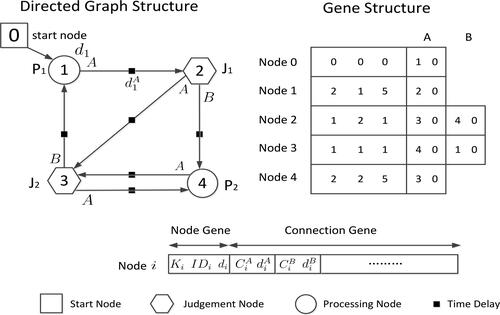
The function of the starting node, as implied by the name, is where the GNP process begins. A judgment node uses an if-then function to select the next node. The processing nodes are used to arrive at a decision. K_i represents the node type; K_i = 0 denotes a starting node; K_i = 1 denotes a judgment node; and K_i = 2 denotes a processing node.

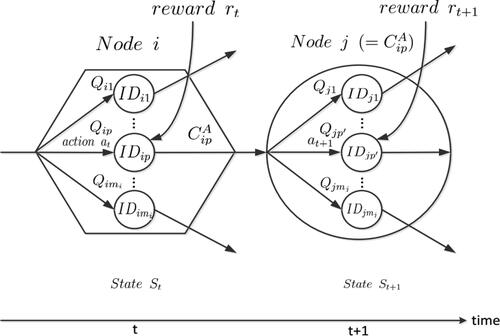
In addition, the judgment and processing nodes usually have an inner sub-node structure, as illustrated in Figure 2. There are two sub-nodes in both, the judgment and processing nodes. The sub-nodes within the judgment node select the next node, and each sub-node can only contain one function. The sub-nodes in the processing node generate decisions. For each sub-node in a judgment or processing node, the Q-value decides the node to be selected next. The Q-value indicates the ‘state’ of the node; for instance, in the judgment node in Figure 2, the sub-nodes $I{D}_{i1}$ and $I{D}_{i2}$ have their own Q-values of $Q_{i1}$ and $Q_{i2},$ respectively. The sub-node with the highest Q-value is selected. If node $I{D}_{i1}$ is selected, the judgment node is in state $I{D}_{i1}.$ During the refinement of GNP passing through the judgment node i, the sub-node $I{D}_{i1}$ will be selected. The Q-value of a processing node is the same as that of a judgment node. The Q-value of each node is determined by SARSA(λ) reinforcement learning, as discussed in detail later. Another useful parameter is the A-value that exists only in the processing node and has the decision-making function. During the evolution of GNP, the A-value is calculated for each state. Subsequently, based on whether the A-value is higher or lower than the threshold, a decision is made (buy or sell). If the condition is not satisfied, the next node is selected.

Figure 2. Inner structure of judgment and processing nodes.

Source: drawn by authors with the help of R software.

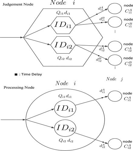
To control the number of nodes to be included during refining, a parameter called the time delay d_i is introduced. There are three types of time delays in our model: the time delay during the transition from one node to the next, the time delay in the judgment node, and the time delay in the processing node. Here, the time delay between nodes is set to zero; the delay at the judgment node is set to one unit; and the delay at the processing node is set to five units. Subsequently, the maximum unit time for the refining process is set to five. When the refining process takes more than five units to complete, it is terminated. Therefore, the maximum number of judgment nodes is five; thus, only one processing node can be included within a single process.

3.2. Evolution process of GNP

As in the GA or GP, one GNP population includes a predefined number of GNP individuals. Each GNP individual represents a solution to the problem. Based on the fitness value of each individual, better individuals are more likely to be selected as the parents of offspring individuals. Crossover and mutation are used as the evolution operators.

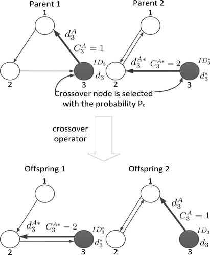
The crossover operator selects two GNP individuals and then exchanges their nodes, as illustrated in Figure 3. The node for any particular GNP individual is selected with probability p_c, and a new individual is generated by this operator as the next generation.

Figure 3. Illustration of the crossover operator.

Source: drawn by authors with the help of R software.

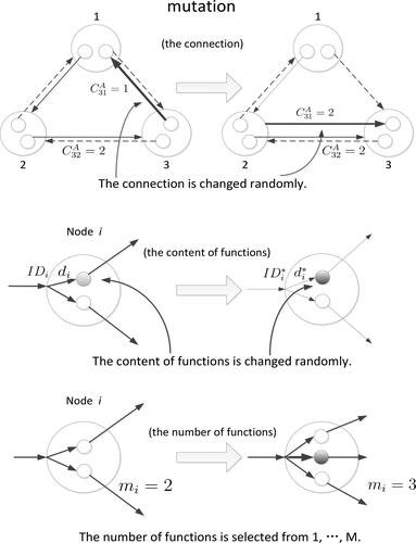
The mutation operator can alter the structure of GNP. When one of the GNP individuals is selected, three types of mutations can be executed: connection change, parameter change, and node function change. As shown in Figure 4, a connection change results in a connection, which is selected with the probability p_m of being reconnected to another node. In a parameter change, the Q-value of a sub-node selected with probability p_m will be altered. A node function change alters the function of the selected sub-node.

Figure 4. Illustration of the mutation operator.

Source: drawn by authors with the help of R software.

3.3. Reinforcement learning: SARSA(λ) algorithm

SARSA is a popular on-policy temporal difference control learning algorithm that has been widely used in several control tasks. This algorithm has a performance superior to that of off-policy algorithms when the space of all possible actions is low-dimensional and discrete. As an on-policy algorithm, it updates function values strictly on the basis of the experience gained from executing some policy. The update function of the SARSA algorithm is defined as follows: $$Q(s,a)\leftarrow Q(s,a)+\alpha \left(r+\gamma Q(s^{\prime },a^{\prime })-Q(s,a)\right),$$ where $s^{\prime }$ is the next state and $a^{\prime }$ is the next action.

Eligibility traces are basic mechanisms of reinforcement learning. They not only bridge temporal difference (TD) methods to Monte Carlo methods, but also mark the memory parameters associated with the eligible event to undergo learning changes. Therefore, from a reverse perspective, an eligibility trace is a temporary record of the occurrence of an event. Almost any temporal difference method, such as Q-learning or SARSA, can be combined with eligibility traces to obtain a more general method that learns more efficiently. The eligibility trace version of SARSA will be called SARSA(λ). The main idea of SARSA(λ) is to apply the TD(λ) prediction method to state-action pairs rather than to states. Thus, a trace is needed not only for each state, but also for each state-action pair. SARSA(λ) is an on-policy algorithm, implying that it approximates $Q^{\pi }(s,a),$ the action values for the current policy π, and then improves the policy gradually based on the approximate values for the current policy. The update rule of the SARSA(λ) algorithm is defined as follows: $$Q_{t+1}(s,a)\leftarrow Q_t(s,a)+e_t(s,a){\delta }_t,$$ where $${\delta }_t\leftarrow \alpha \left(r_{t+1}+\gamma Q_t(s_{t+1},a_{t+1})-Q_t(s_t,a_t)\right).$$

α is the learning rate; the eligibility traces $e(s_t,a_t)$ of all state-action pairs at time-step t can be defined as: $$e_t(s,a)\leftarrow \{\begin{array}{cc}\gamma \lambda e_{t-1}(s,a)+1\hfill & \text{if}\mathrm{}(s,a)=(s_t,a_t)\hfill \\ \gamma \lambda e_{t-1}(s,a)\hfill & \text{otherwise}\hfill \end{array}\hspace{1em}\mathit{for}\hspace{1em}\forall s\in S,\forall a\in A(s).$$

For more details, the standard version of this algorithm with the aforementioned eligibility traces is illustrated in Algorithm 1.

Algorithm 1. The SARSA(λ) Algorithm with Eligibility Trace Replacement

Initialize Q(s, a) arbitrarily and $e(s,a)=0$ for all s, a;

repeat {for each episode}

 Initialize s;

 Choose a from s using policy derived form Q;

 repeat {for each step of episode}

  Take action a, observe reward r, $s^{\prime };$

  Choose $a^{\prime }$ from $s^{\prime }$ using policy derived form Q; $$\delta \leftarrow r+\gamma Q(s^{\prime },a^{\prime })-Q(s,a);$$

  $e(s,a)=1$ {replacing traces};

  for all s, a do $$Q(s,a)\leftarrow Q(s,a)+\delta e(s,a);$$ $$e(s,a)\leftarrow \gamma \lambda e(s,a);$$    end for $$s\leftarrow s^{\prime },a\leftarrow a^{\prime };$$   until state s is terminal  until

3.4. Trading strategy in GNP combined with SARSA(λ) learning

To determine an appropriate and effective trading strategy, the basic structure of GNP must be adjusted. In this section, GNP is combined with the SARSA(λ) algorithm to construct an optimal strategy superior to other traditional methods.

3.4.1. Judgment node functions

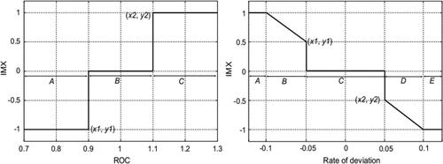
The functions within judgment nodes are defined according to the trading strategies applied during daily transactions. In this study, six indicators were selected for the functions: moving average (MA), relative strength index (RSI), rate of change (ROC), volume ratio, gold cross, and moving average convergence and divergence (MACD) cross. Each of these indicators can be calculated using the closing price over a long or short time period. For example, MA can be calculated using 5 days, 13 days, or 26 days of data. Each technical indicator has its own importance index (IMX) function, which is used to select the next node.

As shown in Figure 5, the x-axis of each chart denotes the index value, and is split into several segments, which are used to select the next node. The y-axis denotes the IMX value, which is a function of the index. IMX is used for the processing node. To illustrate the complete process, consider the following example: if the function in the judgment node is the ROC, and the value of this index is 1.2, according to the IMX chart, the judgment result is C and the IMX value is 1. Then, the next value is $C_{i1}^c,$ and the IMX value is stored to calculate the A-value.

Figure 5. IMX function.

Source: drawn by authors with the help of R software.

3.4.2. Processing node

The processing node is used for making decisions. The procedure is illustrated in Figure 6.

Figure 6. An example of node transition.

Source: drawn by authors with the help of R software.

1. Before arriving at the processing node, several IMX values were already stored while passing through the judgment node. If the current node is the processing node, then the A-value is calculated by averaging the IMX values: $$A_t=\frac{1}{\left|I^{\prime }\right|}\sum _{i^{\prime }\in I^{\prime }}IMX(I^{\prime }),$$

where $I^{\prime }$ is the judgment node set, which includes the previously visited node. $i^{\prime }$ is the judgment node in $I^{\prime }.$

1. The A-value is compared to the threshold to determine whether to buy or sell. If the current sub-node is a buying node, $A_t\ge a_{ip},$ and money is available, then a buying decision can be made. Otherwise, no action is taken. If the current sub-node is a selling node, A_t < a_ip, and stock is available, then a selling decision can be made. Otherwise, no action is taken.

2. The procedure keeps transferring to the next node until the time limit is exceeded.

3.5. Brief explanation of the GNP-SARSA(λ) trading strategy

As the details of the GNP-SARSA(λ) learning model and the associated trading strategy have been introduced, the overall GNP-SARSA(λ) method is discussed.

The GNP-SARSA(λ) algorithm can be considered a ‘technical’ method of trading. It is different from traditional methods because it combines several common indicators, while traditional methods usually include only one indicator. A trading strategy based on the GNP-SARSA(λ) algorithm can combine evolutionary and reinforcement learning methods to find optimal solutions to the model, that is, to determine the optimal strategy for trading. The strategies are stored during the training period and subsequently used to guard the trading, in particular, those of the agents in the ASM in this study.

4. Agent-based stock market model

4.1. Model of agents

In this study, the artificial market includes three types of agents: rational agents, technical agents, and noise agents. Each type of agent has its own wealth, risk preference, and predictive model. Adopting the assumption in the research of Chen and Yeh (2001) that all investors have the same constant absolute risk aversion utility function, $$U(W_i)=-\hspace{0.17em}\text{exp}\hspace{0.17em}(-{\omega }_i{W}_i),$$ where W_i and ω_i are the wealth and risk aversion coefficient of agent i, respectively. The agent’s wealth is composed of two types of assets: money (m_i) and stocks (S_i); thus the wealth of each agent at time t is $W_{i,t}=m_{i,t}+S_{i,t}\times p_t.$ Under the normal distribution assumption of stock price and dividends, the optional position of the risk assets is $po{s}_t^i=\frac{E(p_{t+1,i}|I_t)/p_t-1-r}{{\omega }_i{\sigma }_t^2}.$

4.1.1. Rational agents

A rational agent believes that the expected price of the stock is decided by the dividend discount model (DDM). The rational stock price is the discount of these future dividends based on the DDM: $$E(p_{t+1,i}|I_t)=\frac{d_t/r}{{\omega }_i},$$ where $p_{t+1,i}$ is the ith agent’s expectation of the price at time t + 1; I_t contains all the information in period t; r is the constant cost of equity capital; and ω_i is the agent’s risk aversion coefficient. The risk aversion coefficient is introduced in the DDM to reflect the impact of risk preference on price expectation. d_t is the dividend in period t, and it follows a random walk process, namely $d_t=\alpha d_{t-1}+e_t,$ where e_t are i.i.d. random variables each with zero mean and variance ${\sigma }_t^2.$

In each period, rational agents can obtain the dividend information on the stock and can calculate the rational price of the stock and the optimal position for their own risk assets. Upon comparing their optimal position with the current position, they buy or sell the stock at the predicted price to satisfy the optimal position.

4.1.2. Technical agents

Technical agents usually use historical market data to forecast the trend of the price. Common indicators such as the RSI and MACD are used to determine the trading strategy. As introduced in the previous section, the GNP model can be thought of as a technical method for investors. The advantage of using a GNP model for the trading strategy is that it not only combines model indicators, but also specifies thresholds for trading.

Moreover, as with the GA and GP models, GNP also has evolution features to describe the adaptation of the agents. These advantages render GNP suitable for agents who use technical analysis in the proposed artificial market.

4.1.3. Noise agents

The existence of noise traders has been shown in many previous studies. Noise traders are irrational investors who do not adopt common stock pricing methodologies, technical analysis methods, or portfolio optimization. In this study, the definition of Black (1986) is adopted for noise traders: such investors, with no access to inside information, irrationally act on noise as if it were information that would give them an edge. Under this definition, it is assumed that a noise trader has a biased expectation of the stock price (De Long et al., 1990), that is, the bias of the expected price follows a normal distribution with constant variance: $${\rho }_t\sim N({\rho }^{*},{\sigma }_{\rho }^2).$$

Thus, the expected price can be described as $$E(P_{t+1}^n)=E(P_{t+1})+{\rho }_t,$$ where $E(P_{t+1}^n)$ is the expected stock price of noise traders, and $E(P_{t+1})$ is decided by the DDM.

4.2. Model of the pricing mechanism

The pricing mechanism is also an important factor in the series data of the stock price and the returns for each agent. In some papers, the pricing mechanism is called a specialist. It collects bids, offers a price and volume, and then chooses a knockdown price. The knockdown price reflects the demand and supply of the market. Four types of mechanisms were proposed in early research (LeBaron, 2006). These mechanisms were: temporary market equilibrium, price impact function, order book, and matching. In this study, a pricing mechanism referred to as call auction was used. With call auction, after each agent bids a price and direction, the mechanism collects all bids and chooses a knockdown price that satisfies several conditions. In this study, the condition was imposed to maximize the trading volume. This pricing mechanism is used to choose the start price of each day’s trading in the Shanghai and Shenzhen Exchanges. The process of this mechanism is: (1) collect all bids in the buying/selling direction; (2) order all bids by their bid price; (3) check each price in the orders, and find out how much trading volume can be achieved at each price (the achievable trading volume is the minimum aggregate volume in the buying and selling directions); and (4) choose the price which can achieve the maximum trading volume. This mechanism can be represented by the formula: $$p=\arg \{\underset{p_c\in \theta }{\max }\min (\sum _{p_i\ge p_c}{h}_{b,p_i},\sum _{p_j\le p_c}{h}_{b,p_j})\},$$ where θ is the set of all call prices; $h_{b,p_i}$ is the share at price p_i to buy; $h_{s,p_j}$ is the share at price p_j to sell; and p_c is the price in the price set θ.

4.3. Model of agent adaptation

In the proposed model, adaptation of the agents is represented by changing their predictive method. Chen and Yeh (2001) assumed that each agent changes the predictive model with a certain probability, given by $p_{i,t}=\frac{R_{i,t}}{N},$ where $R_{i,t}$ is the rank of the agents in order of returns. Thus, the traders who are ranked at the top have a lower probability of changing their model. However, this setting assumes that agents can get other agents’ returns instantly, an assumption which we think does not reflect reality. Because the agents’ returns are stored as private information, they will not share this information with other agents; hence, the rank $R_{i,t}$ is in fact unavailable. In this study, it is assumed that rational agents and noise agents never change their predictive method, but that the technical agents check the returns of the current predictive method according to the GNP strategy. Agents can check the returns of the GNP strategy held in the past n days. The return is $r=\frac{W_{t,i}-W_{t-n,i}}{W_{t-n,i}}.$ Each agent has an expectation that the return follows the expression $r_i^e=r_f+{\theta }_r,$ where r_f is the risk-free rate and θ_r is the risk premium for the risk asset, which can be approximated by ${\theta }_r\sim N(\lambda r_f,{\sigma }_r).$ The parameter λ is specified to control the risk premium. If the return of the current GNP strategy is below expectations, then λ is used to compare the returns of the current GNP strategy with those of other alternative GNP strategies, until a GNP is found that is higher than the agent’s expectation. After that, agents use the newly assigned GNP strategy as their predictive method.

4.4. Knowledge base of GNP

In this study, the GNP strategies are stored in a knowledge base, which can easily be accessed by technical agents. This knowledge base dynamically updates during transactions. The GNP strategies are updated every n periods with the latest price and volume data. Each agent can use the newly generated GNP strategies after they are added to the knowledge base. This dynamical updating can also be considered as a type of agent adaptation.

5. Simulation design and result analysis

Different expectations of risky assets form the relationship between transaction supply and demand for traders in the financial market. In an ASM, each type of agent holds a different expectation, and even those of the same type have different risk preferences. The following problems will be discussed through simulations for this novel model:

1. The first problem is the character of the generated price time series in the ASM. Does the price and return series follow a normal distribution? Does it have a heavy tail?

2. The second problem is regarding how a change in market forces impacts the market. Do changes of forces lead to more volatility?

5.1. Simulation design

Simulation design usually refers to the setting of the elements (agents, pricing mechanism, and so on) in an ASM. This set includes the agents’ characteristics such as their assets, risk preferences, and predictive methods. The settings for the market include the number of each type of agent, the risk-free rate, and the total trading days. In this study, there is an extra setting for the GNP-SARSA(λ) model. These important parameters, which were carefully tuned to ensure a smooth running of the market, are listed in Table 1.

Table 1. Parameter settings.

Parameters	Value	Parameters	Value
Noise traders	400/1000/100/100	Technical Traders	400/100/1000/100
Fundamental traders	400/100/100/1000	Risk-free rate	0.03
Alpha (dividend process)	1	Sigma (dividend process)	0.001
Rho (noise agent)	N(0,0.1)	Lambda	0.1
Theta (agent adaptation)	N(0.003,0.000001)	Days of changing the model	20
Initial money of agent	20000	Initial shares of agent	1000
Risk aversion	N(1,0.001)	Number of GNPs	500
Alpha (Sarsa(λ))	0.1	Gamma (Sarsa(λ))	0.4
Lambda (Sarsa(λ))	0.9
GNP parameters	Value	GNP parameters	Value
Number of individuals	300	Judgment Node	30
Process node	20	Number of Subnodes	2
Crossover rate	0.2	Mutation rate	0.3

Source: calculated by authors via R software.

To establish a GNP knowledge base, real price series data are used to generate GNP strategies. To ensure typical strategies, Shanghai A-Stock Exchange Index and trading volumes were used for the training data. The period of data ran from January 4, 2013 to December 30, 2016. In total, 500 GNP strategies were generated for the initial knowledge base. Agents could choose and compare GNPs as their prediction models.

To study the influence of the changes in market forces, four experiments were separately conducted. Each experiment was executed for 2000 trading days. The generated stock prices, bonus, and the holding of each agent were recorded in text files. The data from the first 500 trading days were dropped to allow time for transition into a smooth state. The remaining 1500 trading days were used for the research.

5.2. Simulation result and analysis

5.2.1. Character of price series data

To answer the first question, the characters of price series data in four experiments were tested. Each of these four experiments presents different forces with a different number of agents in the market. For example, in the balanced-forces market, the number of each type of agents is equal; in our experiment, 400 agents of each type were used. In the noise-agent-dominated market, the number of noise agents is much larger than the other two types of agents; in our experiment, there are 1000 noise agents, 100 technical agents, and 100 fundamental agents. The technical-agent-dominated market and fundamental-agent-dominated market are arranged, similar to the noise-agent-dominated market.

Figures 7 and 8 show the price and return time series data of the four types of markets. Tables 2 and 3 present descriptive statistics for these four prices and return time series.

Figure 7. The price time series of the four market types.

Source: drawn by authors with the help of R software.

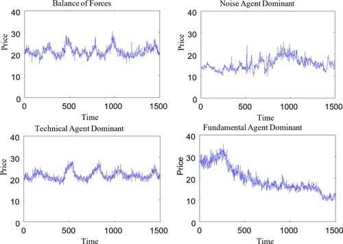
Figure 8. The return time series of the four market types.

Source: drawn by authors with the help of R software.

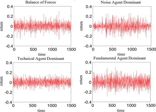
Table 2. Descriptive statistics of price for the four price time series.

Statistics types		Balance forces	Noise agent dominant	Technical agent dominant	Fundamental agent dominant
Mean		21.09	15.50	21.58	13.54
Sigma		2.11	2.65	1.96	2.85
Skewness		0.73	0.63	0.82	0.33
Kurtosis		3.74	3.02	3.66	2.27
Shapiro-Wilk	Stat	0.97	0.969	0.958	0.975
	P-value	< 0.0001	< 0.0001	< 0.0001	< 0.0001
Kolmogorov-Smirnov	Stat	0.06	0.07	0.08	0.05
	P-value	< 0.0100	< 0.0100	< 0.0100	< 0.0100
Cramer-von Mises	Stat	1.79	2.35	3.13	1.47
	P-value	< 0.0050	< 0.0050	< 0.0050	< 0.0050
Anderson-Darling	Stat	11.10	14.05	18.24	10.05
	P-value	< 0.0050	< 0.0050	< 0.0050	< 0.0050

Source: calculated by authors via R software.

Table 3. Descriptive statistics of return for the four price series.

Statistics types		Balance forces	Noise agent dominant	Technical agent dominant	Fundamental agent dominant class
Mean		−0.000023	0.000116	−0.000014	−0.000335
Sigma		0.059975	0.065549	0.058708	0.038028
Skewness		−0.026452	−0.049936	−0.046583	0.024956
Kurtosis		4.611933	5.304814	5.119004	3.376879
Shapiro-Wilk	Stat	0.99	0.96	0.98	1.00
	P-value	< 0.0001	< 0.0001	< 0.0001	0.03
Kolmogorov-Smirnov	Stat	0.03	0.08	0.03	0.02
	P-value	< 0.0100	< 0.0100	< 0.0100	0.05
Cramer-von Mises	Stat	0.40	3.66	0.43	0.20
	P-value	< 0.0050	< 0.0050	< 0.0050	0.01
Anderson-Darling	Stat	2.62	20.36	3.18	1.04
	P-value	< 0.0050	< 0.0050	< 0.0050	0.01

Source: calculated by authors via R software.

Figure 7 shows the price trends in the four types of markets. It is clearly observed that the balanced-forces market and the technical market have similar trends, indicating the influence of technical agents on market price trends. Table 2 displays the descriptive statistics and tests for normality. In this study, three methods for testing normality show that the price time series data in these four scenarios do not follow a normal distribution.

The return series is derived from $r_t=\hspace{0.17em}\text{ln}\hspace{0.17em}(P_t)-\hspace{0.17em}\text{ln}\hspace{0.17em}(P_{t-1}).$ It can be observed in Figure 3 that none of the four normal testing methods are normally distributed. Furthermore, a heavy tail is illustrated by the kurtosis statistic results. In the balanced-forces market, noise-agent-dominated market, and technical-agent-dominated market, the kurtosis is much larger than three, which is associated with a normal distribution. The kurtosis value of the fundamental-agent-dominated market is modestly smaller than those of the other three market types while displaying some type of heavy-tail characteristic.

5.2.2. Impact of changing market forces

As described previously, this research considers four types of markets. Three of the markets are dominated by one type of agent. In the fourth market, the forces of agents are equal. This research also focuses on the impacts of price variation. Figure 9 shows the price and bonus trends in the four markets.

Figure 9. Trends of prices and bonuses in the four markets.

Source: drawn by authors with the help of R software.

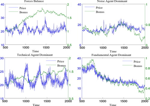
First, the fundamental-agent-dominated market is considered. In this type of market, fundamental agents determine the bonus series of the risk assets and the real price of the risk assets by the dividend discount model. The only differences between agents are their risk preferences, which impact the optimal position of their risk assets. In Figure 9, it is clear that the price series and bonus series have a high correlation. For the domination of fundamental agents, the price trend cannot significantly differ from the bonus trend.

The noise-agent-dominated market is the same as the fundamental-agent-dominated market; the price series is close to the bonus series, but it varies more than that of the fundamental-agent-dominated market. This can be attributed to the design of the noise agent. The difference between a noise agent and a fundamental agent is that there is a bias (ρ_t) in the expectation of price for a noise agent. The bias follows a normal distribution ${\rho }_t\sim N({\rho }^{*},{\sigma }_{\rho }^2).$

For the technical-agent-dominated market and the balanced-forces market, the situation changes. Figure 9 shows that price trends have their own pattern and are no longer related to the bonus. The similarity between these two price trends indicates that technical agents play an important role in price generation.

To measure the correlation between price and bonus trends in these four markets, the linear correlation coefficients were calculated. Table 4 shows the results. From this table, the conclusion can be drawn that there is a strong relationship between price and bonus trends in markets dominated by fundamental agents and noise agents. However, the relationship is very weak in the other two markets.

Table 4. Correlation between price and bonus trends.

	Balanced forces	Noise agent	Technical agent	Fundamental agent
		Dominant	Dominant	Dominant
Coefficient	0.070	0.553	0.031	0.983

Source: calculated by authors via R software.

There is significant research proving that excess volatility exists in financial markets. For instance, Shiller (1981) proposed a relationship between the volatility of price and dividends. In this study, our focus is on how changes in market forces impact excess volatility, for which two steps are proposed. The first step is to prove that excess volatility exists in ASM price series. Based on the results, the second step is to test whether there is a difference in the excess volatility between these four markets.

The basic method of this research is similar to the one used by Shiller (1981). The real price is obtained from the dividend series using $p_t^d=d_t/r_f.$ Assuming that the risk-free rate r_f is constant, d_t is a random walk process. Next, the 1500 trading days are separated into 30 periods. Each period includes 50 trading days. The volatilities of p_t and $p_t^d$ in each period are calculated. Finally, analysis of variance (ANOVA) methods are used to test whether there is a distinct difference in volatility between p_t and $p_t^d.$

The ANOVA analyses for these four markets reject the hypothesis of no difference in volatility between p_t and $p_t^d,$ as shown in Table 5, implying that there are significant differences between the volatilities of p_t and $p_t^d.$ Therefore, in these four types of markets, the volatility of the market price (p_t) is significantly larger than the dividend discount price ($p_t^d$), which proves the existence of excess volatility.

Table 5. ANOVA analysis of excess volatility.

Source	DF	Sum of squares	Mean square	F value	Pr >F
Panel A: Balanced forces market
Model	1	2.686	2.686	16.330	0.000
Error	58	9.543	0.165
Corrected total	59	12.229
Panel B: Noise agent dominated market
Model	1	3.634	3.634	15.690	0.000
Error	58	13.433	0.232
Corrected total	59	17.068
Panel C: Technical agent dominated market
Model	1	1.610	1.610	11.330	0.001
Error	58	8.243	0.142
Corrected Total	59	9.853
Panel D: Fundamental agent dominated market
Model	1	1.022	1.022	6.040	0.017
Error	58	9.822	0.169
Corrected total	59	10.845

Source: calculated by authors via R software.

In the second step, ANOVA calculates the difference in excess volatility in these four markets. Because the dividend series in each market arise from different random processes, the volatility ratio between the ASM and DDM prices is used to remove these effects; that is ${\kappa }_{i,t}={\sigma }_{i,p_t}/{\sigma }_{i,p_t^d},$ where ${\sigma }_{i,p_t}$ is the volatility of the ASM price and ${\sigma }_{i,p_t^d}$ is the volatility of the DDM price. The ANOVA results of ${\kappa }_{i,t}$ are displayed in Table 6.

Table 6. The ANOVA Analysis Result of κ.

Source	DF	Sum of squares	Mean square	F value	Pr >F
Model	3	0.115	0.038	0.15	0.931
Error	116	30.137	0.260
Corrected Total	119	30.252

Source: calculated by authors via R software.

The results in Table 6 show that the p-value is larger than the 5% confidence level, implying that the null hypothesis cannot be rejected. This also implies that there is no significant difference in volatility among these four markets.

This result is expected; the first step of this study already proved the existence of excess volatility in all four markets, including the markets in which fundamental agents do not dominate. This indicates that excess volatility does not arise only from the dividend process, which is an unstable random walk. A fundamental cause of excess volatility is the difference in the beliefs or expectations of agents regarding the stock price.

6. Concluding remarks

An efficient GNP-SARSA(λ) algorithm for an agent-based artificial financial market was presented and three assertions were evaluated.

First, an ASM with three types of agents was established to study how belief affects stock price trends. The three types of agents consisted of fundamental, technical, and noise agents. Each type of agent was designed with a predictive model for the stock price. This predictive model can be regarded as the beliefs or expectations of the agents themselves. Technical agents represented the traders who use candle charts and other indexes to trade stocks. GNP was also introduced to build a knowledge base for technical agent trading. GNP provides a key advantage in evolutionary features that can be used for agent adaptation.

Second, price trends affected by the market domination of different agents were studied through simulations. It was determined that technical agents can influence the price to deviate from the real price decided by the DDM. However, the price trends in noise-agent-dominated markets and fundamental-agent-dominated markets still approached the real price.

Finally, our ASM was tested for the existence of excess volatility and compared for the four types of markets. The results indicate that the excess volatility is not significantly different in any of these markets. The difference in expectation is the reason for the excess volatility in price.

Disclosure statement

No potential conflict of interest was reported by the authors.

Additional information

Funding

Chen’s work is supported by National Natural Science Foundation of China (No. 71571113), Major Science and Technology Projects in Hunan Province (No. 2018GK1020), and the Fundamental Research Funds for the Central Universities.

References

- Arifovic, J., & Masson, P. R. (2000). Heterogeneity and evolution of expectations in a model of currency crisis. Brookings Institution.
- Arthur, W. B., Holland, J. H., LeBaron, B., Palmer, R., & Taylor, P. (1996). Asset pricing under endogenous expectation in an artificial stock market.
- Bertschinger, N., & Mozzhorin, I. (2021). Bayesian estimation and likelihood-based comparison of agent-based volatility models. Journal of Economic Interaction and Coordination, 16(1), 173–210. https://doi.org/10.1007/s11403-020-00289-z
- Black, F. (1986). Noise. The Journal of Finance, 41(3), 528–543. https://doi.org/10.1111/j.1540-6261.1986.tb04513.x
- Chakole, J. B., Kolhe, M. S., Mahapurush, G. D., Yadav, A., & Kurhekar, M. P. (2021). A Q-learning agent for automated trading in equity stock markets. Expert Systems with Applications, 163, 113761. https://doi.org/10.1016/j.eswa.2020.113761
- Chen, Y., Mabu, S., Hirasawa, K., & Hu, J. (2007). Trading rules on stock markets using genetic network programming with sarsa learning [Paper presentation]. Proceedings of the 9th Annual Conference on Genetic and Evolutionary Computation (pp. 1503–1503). ACM. https://doi.org/10.1145/1276958.1277232
- Chen, Y., Mabu, S., Shimada, K., & Hirasawa, K. (2009a). A genetic network programming with learning approach for enhanced stock trading model. Expert Systems with Applications, 36(10), 12537–12546. https://doi.org/10.1016/j.eswa.2009.05.054
- Chen, Y., Ohkawa, E., Mabu, S., Shimada, K., & Hirasawa, K. (2009b). A portfolio optimization model using Genetic Network Programming with control nodes. Expert Systems with Applications, 36(7), 10735–10745. https://doi.org/10.1016/j.eswa.2009.02.049
- Chen, S. H., & Yeh, C. H. (2001). Evolving traders and the business school with genetic programming: A new architecture of the agent-based artificial stock market. Journal of Economic Dynamics and Control, 25(3–4), 363–393. https://doi.org/10.1016/S0165-1889(00)00030-0
- De Long, J. B., Shleifer, A., Summers, L. H., & Waldmann, R. J. (1990). Noise trader risk in financial markets. Journal of Political Economy, 98(4), 703–738. https://doi.org/10.1086/261703
- Eguchi, T., Hirasawa, K., Hu, J., & Ota, N. (2006). A study of evolutionary multiagent models based on symbiosis. IEEE Transactions on Systems, Man, and Cybernetics. Part B, Cybernetics: A Publication of the IEEE Systems, Man, and Cybernetics Society, 36(1), 179–193. https://doi.org/10.1109/tsmcb.2005.856720
- Frankel, J. A., & Froot, K. A. (1986). Explaining the demand for dollars: International rates of return and the expectations of chartists and fundamentalists. Department of Economics, UCB.
- Hommes, C. H. (2006). Heterogeneous agent models in economics and finance. Handbook of Computational Economics, 2, 1109–1186. https://doi.org/10.1016/S1574-0021(05)02023-X
- Huang, Y., Gao, Y., Gan, Y., & Ye, M. (2021). A new financial data forecasting model using genetic algorithm and long short-term memory network. Neurocomputing, 425(15), 207–218. https://doi.org/10.1016/j.neucom.2020.04.086
- Joshi, S., Parker, J., & Bedau, M. A. (1999). Technical trading creates a prisoner’s dilemma: results from an agent-based model. Computational Finance, 99, 465–479.
- Kirman, A. (1991). Epidemics of opinion and speculative bubbles in financial markets. Money and Financial Markets, 3, 54–368.
- LeBaron, B. (2006). Agent-based computational finance. Handbook of Computational Economics, 2, 1187–1233. https://doi.org/10.1016/S1574-0021(05)02024-1
- LeBaron, B., Arthur, W. B., & Palmer, R. (1999). Time series properties of an artificial stock market. Journal of Economic Dynamics and Control, 23(9-10), 1487–1516. https://doi.org/10.1016/S0165-1889(98)00081-5
- Lettau, M. (1997). Explaining the facts with adaptive agents: The case of mutual fund flows. Journal of Economic Dynamics and Control, 21(7), 1117–1147. https://doi.org/10.1016/S0165-1889(97)00046-8
- Levy H., Levy M., & Solomon S. (2000). Microscopic simulation of financial markets: from investor behavior to market phenomena. Academic Press.
- MacDonald, R., Grauwe, P. D., Dewachter, H., & Embrechts, M. (1994). Exchange rate theory: Chaotic models of foreign exchange markets. The Economic Journal, 104(425), 966. https://doi.org/10.2307/2235001
- Routledge, B. R. (2001). Genetic algorithm learning to choose and use information. Macroeconomic Dynamics, 5(02), 303–325. https://doi.org/10.1017/S1365100501019083
- Sargent, T. J. (1993). Bounded rationality in macroeconomics: The Arne Ryde memorial lectures. OUP Catalogue.
- Shiller, R. J. (1981). Do stock prices move too much to be justified by subsequent changes in dividends? The American Economic Review, 71(3), 421–436.
- Song, G., Xia, Z. Q., Basheer, M. F., & Shah, S. M. A. (2021). Co-movement dynamics of US and Chinese stock market: Evidence from COVID-19 crisis. Economic Research-Ekonomska Istraživanja, 1–17. https://doi.org/10.1080/1331677X.2021.1957971
- Wang, L. M., Xu, Y. Y., & Salem, S. (2021). Theoretical and experimental evidence on stock market volatilities: A two-phase flow model. Economic Research-Ekonomska Istraživanja, 1–25. https://doi.org/10.1080/1331677X.2021.1874459
- Yao, Y. Y., Cai, S. Z., & Wang, H. M. (2021). Are technical indicators helpful to investors in china’s stock market? A study based on some distribution forecast models and their combinations. Economic Research-Ekonomska Istraživanja, 1–25. https://doi.org/10.1080/1331677X.2021.1974921
- Zare, M., Naghshineh Arjmand, O., Salavati, E., & Mohammadpour, A. (2021). An Agent-Based model for Limit Order Book: Estimation and simulation. International Journal of Finance & Economics, 26(1), 1112–1121. https://doi.org/10.1002/ijfe.1839