Does China transmit financial cycle spillover effects to the G7 countries?

Abstract

We use the state space model to describe the financial cycles of China and G7 countries since 1990, and the DY spillover index to quantify the spillover effects of China's financial cycles on G7 countries. We find that China plays the role of a net recipient most of the time. China's financial cycle net spillover index fluctuates widely and is vulnerable to economic events such as the financial crisis. This implies that international capital flows have brought volatility and shocks to the Chinese financial market, such as the Asian financial crisis and the 2008 international financial crisis. In addition, during 2004-2005 and 2014-2015, the G7 countries also suffered from financial cycle spillover from China. The US received most of the financial cycle spillover from China, followed by Canada, Germany, and Italy.

Keywords:

• financial cycle
• spillover effect
• state-space model
• DY spillover index

JEL CLASSIFICATION:

• C32
• E32

1. Introduction

In periods of financial instabilities, like the 2008 global financial crisis, volatility transmission becomes a cause of concern to financial analysts, investors, policymakers, regulators, and researchers, who seek to ascertain the cross-border sources of risk of financial investment. After the 2008 financial crisis, the behavior of the financial cycle and cross-border contagion to other economies has attracted the attention of economists. Prominent in this research is the inability of traditional business cycle theories to explain or predict the global financial crisis, which was catalyzed by the limited understanding of the risk of investment in asset-back securities. In the aftermath of the crisis, world organizations have paid increasing attention to the financial cycle, and have highlighted its importance for the allocation of financial resources, risk management, and macro-prudential regulation.

Most financial cycle peaks are synchronized with the time of the global financial crisis (Borio, 2014; Drehmann et al., 2012). The credit boom means that the regional financial cycle reaches its peak. During this period, the bankruptcy of a company with extensive financial connections will trigger a systemic financial crisis. When Krishnamurthy and Muir (2017) studied the behavior of credit prices and quantities, they showed that the expansion of credit supply is a precursor to a crisis. Kumhof et al. (2015) believe that increasing inequality will promote credit prosperity and trigger a banking crisis. In addition, the research results of Miranda-Agrippino and Rey (2020) show that before the outbreak of the financial crisis, global financial institutions assumed more external risks.

The current literature has not precisely defined the financial cycle, since different researchers endow it different connotations from different angles. The most widely accepted definition of the finance cycle is presented by Borio (2014). Prominent academic works seek to characterize the financial cycle empirically (Li et al., 2020; Schüler et al., 2015, 2017); estimate its interactions with the business cycle (Claessens et al., 2012; Uddin et al., 2020), and examine its ability to predict financial crises and economic activities (Ghosh, 2020; Ng, 2011). Furthermore, an increasing body of literature emphasize the need for a deeper understanding of the financial cycle (Li et al., 2020; Rey, 2015; Sukharev, 2020). Key conclusions drawn from the above-mentioned literature are as follows. First, financial cycles evolve and are longer, more asymmetric and ampler than business cycles. Second, their peaks are vulnerable to financial crises, which help detect risks in advance. Third, financial cycles are best described by the behavior of credit and property prices. Credit expansion is a leading indicator of the financial crisis (Borio, 2014; Schularick & Taylor, 2012). Therefore, the expansion and contraction of credit and financial asset prices are good indicators of the boom and bust of the financial cycle. Building on the financial cycle literature, our research defines the financial cycle as cyclical fluctuations caused by the expansion and contraction of credit and asset prices.

Economists mostly use the turning-point analysis and frequency-based filter methods to capture the financial cycle (Borio, 2014; Drehmann et al., 2012). Recent research has produced a variety of methods for measuring financial cycles. In this regard, Schüler et al. (2015) combine a multivariate spectral approach with a time-varying aggregation to characterize financial cycles. Strohsal et al. (2019) estimate autoregressive moving average (ARMA) models for standard financial cycle indicators, and they use the estimated models to compute their corresponding frequency domain representations.

Several recent financial crises have spread rapidly around the world, proving that the spillover effects of financial assets across regions cannot be ignored. In recent years, scholars (Diebold & Yilmaz, 2012; Kolia & Papadopoulos, 2020; Shen et al., 2021) have been keen to use different capital markets financial variables construct spillover models to quantify spillover effects between different capital markets. Looking back on the previous literature, there are abundant researches on the spillover relationship among major financial markets such as the stock market, bond market, foreign exchange market, and currency market.

In this paper, we utilize a Kalman filter model – which uses a powerful iterative algorithm – for parameter estimation and inference about unobserved variables in linear dynamic systems. Thus, we construct a time-varying parameter state-space model to characterize the financial cycles. An advantage of this approach is that, unlike other approach that rely on observable variables, the state-space model combines unobserved variables with observable variables, and it obtains coefficient estimates of the financial cycle model. In addition, we refer to the research of Diebold and Yilmaz (2012), who use the generalized variance decomposition method to measure risk contagion. This method later became widely known as the ‘DY spillover index’. In principle, this method is applicable to various risk contagion scenarios. We use the DY spillover index to quantify the spillover effects of the financial cycle.

2. China’s financial cycle

2.1. Definition of the financial cycle

To gain a better understanding of the financial cycle concept, it is necessary to gauge the differences and similarities between the financial cycle and the business cycle. The business cycle generally refers to a regular expansion and contraction of real economic activity – e.g., employment and gross domestic product – around the general trend of economic development. On the one hand, both the financial cycle and the business cycle reflect the cyclical fluctuations in the macroeconomy, and the financial cycle has a predictive power of the business cycle. As a result, the two variables share similar information contents about the macroeconomy.

A more distinct definition of financial cycle is proposed in this study. Building on the experience of prior research, this study defines financial cycle as cyclical fluctuations caused by an expansion and contraction of credit and financial asset prices such as credit growth, as well as equity and house prices. Financial cycle can be measured as the dynamic trend in credit growth and financial asset prices at different stages of economic fluctuations. It can be seen from the experience of recent financial crises that financial instability is generally triggered by drastic changes in credit and financial asset prices (Borio, 2014). Thus, the financial cycle can be driven or attenuated by macroprudential and monetary policies (Li et al., 2018; Schularick & Taylor, 2012; Schüler et al., 2015).

There are some differences between our definition of the financial cycle and previous literature. Before the 2008 financial crisis, scholars who studied the financial cycle were concerned about the currency and credit cycle, which can be regarded as the initial stage of the financial cycle. The definition of the financial cycle in this paper focuses on credit and financial asset prices. We used credit to private non-financial sector to represent credit, and short-term interest rate, real effective exchange rate, share price index, and the real house prices index to represent financial asset prices.

2.2. China’s financial cycle spillovers

China’s government has formulated relevant policies that have affected China’s financial cycle spillovers. For example, fluctuation from the renminbi (RMB) exchange rate and monetary policy can lead to the unidirectional spillovers in China’s financial cycle volatility. Hammoudeh et al. (2014) found that China’s monetary policy has an important impact on international commodity price indexes. Monetary policies of the dominant countries produce large financial spillovers to the rest of the world. Therefore, it is reasonable to hypothesize that:

Hypothesize 1. China’s financial cycle has spillover effects on the financial cycles of other countries.

Credit scale, interest rate, RMB exchange rate, stock market and real estate market are vulnerable to the impact of national policies and the outbreak of the financial crisis. Krishnamurthy and Muir (2017) show that expansion of credit supply occurs before financial crises. There is no doubt that interest rates are closely related to national policies. When studying the spillover effect of RMB exchange rate, Wei et al. (2020) pointed out that the spillover effect of RMB exchange rate is inevitably affected by adjustment of exchange rate mechanism and global economic and political events, especially during the epidemic period. Research by Mazur et al. (2021) showed that stock values and real estate values fell sharply during the pandemic. Therefore, it is reasonable to hypothesize that:

Hypothesize 2. China’s financial cycle spillover effects are sensitive to special events.

Wang et al. (2020) studied policy uncertainty and stock market behavior and found that China is a net recipient of uncertainty risk and stock market risk, and its role is limited. Xu et al. (2019) discussed the spillover effects of oil and stock markets and concluded that the Chinese stock market is a net recipient. McIver and Kang (2020) analyzed the spillover effects of stock market returns in the United States and financial countries, and pointed out that China and most of the BRICS countries act as net receivers. Therefore, it is reasonable to hypothesize that:

Hypothesize 3. China is the recipient of the spillover effects of the financial cycle.

3. Methodology

3.1. Data

There is no consensus how to measure the state of the financial sector. A multivariate approach that relies on a range of macro-financial indicators provides the best-suited method for obtaining a financial cycle estimate (Schüler et al., 2015). This method allows to obtain a financial cycle index with different aspects of a financial system. In this section, a system of indicators for measuring the financial cycles in China and the G7 countries will be constructed. These indicators are similar to those proposed by Claessens et al. (2012) and extend through 2018. Table 1 summarizes the variables, the measurements, the sample of countries, and the sources of information. As we analyzed in the first part, we are going to comprehensively evaluate the financial cycle from the five variables of credit and financial asset prices. These five variables are credit growth, interest rates, exchange rates, equity price, and housing prices.

Table 1. Database and countries list.

Variable	Measurement	Source
Credit	Credit to Private non-financial sector deflated using CPI	BIS
Interest rate	Short-term interest rate	OECD
Exchange rate	Real Effective Exchange Rate	IFS
Equity price	Share Price Index	OECD
House price	The real house prices index	OECD
Sample countries: China (CHN), Canada (CAN), France (FRA), Germany (DER), Italy (ITA), Japan (JPN), United States (US), and United Kingdom (UK).

Note: OECD, BIS, and IFS represent the Organization for Economic Co-operation and Development statistical database, Bank for International Settlements database, and International Financial Statistics of International Monetary Fund, respectively.

Source: The Authors.

3.2. Financial cycle measurement

First, we construct an aggregate measure of the financial cycle index, which consists of credit growth, interest rate, exchange rate, equity price, and house price. The financial cycle index calculated by Equation (1)(1) $${\mathit{FCI}}_t={\sum }_i^5{w}_{it}\times (q_{it}-{\overline{q}}_{it})/{\overline{q}}_{it}$$(1) is a composite measure of the conditions in financial markets. The financial cycle index (FCI) is defined as (1) $${\mathit{FCI}}_t={\sum }_i^5{w}_{it}\times (q_{it}-{\overline{q}}_{it})/{\overline{q}}_{it}$$(1) where $q_{it}$ is the price of asset $i$ (indicate credit, interest rate, exchange rate, equity price, and house price) in period $t,$ ${\overline{q}}_{it}$ is the long-run trend or equilibrium value of the price of asset $i$ in period$\mathrm{}t,$ and $w_{it}$ are the relative weight allocated to asset $i$ in FCI. We use the Hodrick-Prescott Filter (H-P henceforth) to obtain the long-run trend or equilibrium value of the variables. Thus, $(q_{it}-{\overline{q}}_{it})/{\overline{q}}_{it}$ is the relative gap of the variable. To quantify the effects of fluctuations in each variable on the financial cycle, the weights of FCI are computed by $w_{it}=z_{it}/{\sum }_{i=1}^5\left|z_{it}\right|,$ where $z_{it}$ is the time-varying coefficient estimated by the state-space model. Before estimating the state space model, we perform unit root tests on these variables. The test results show that the null hypothesis that there is a unit root is rejected.

We formulate a state-space model that features the time-varying weight of financial variables, $z_{it}.$ The state space model features of the measurement equation (Equation 2(2) $$y_t={\beta }_0+{\sum }_{k=0}^t{\beta }_k{y}_{t-k}+{\sum }_{j=0}^t{z}_{1j}{\mathit{Credit}}_{t-j}+\mathrm{}{\sum }_{j=0}^t{z}_{2j}{\mathit{Interest}}_{t-j}+{\sum }_{j=0}^t{z}_{3j}{\mathit{Exchange}}_{t-j}+{\sum }_{j=0}^t{z}_{4j}{\mathit{Equity}}_{t-j}+{\sum }_{j=0}^t{z}_{5j}{\mathit{House}}_{t-j}+{\mu }_t$$(2) ) (2) $$y_t={\beta }_0+{\sum }_{k=0}^t{\beta }_k{y}_{t-k}+{\sum }_{j=0}^t{z}_{1j}{\mathit{Credit}}_{t-j}+\mathrm{}{\sum }_{j=0}^t{z}_{2j}{\mathit{Interest}}_{t-j}+{\sum }_{j=0}^t{z}_{3j}{\mathit{Exchange}}_{t-j}+{\sum }_{j=0}^t{z}_{4j}{\mathit{Equity}}_{t-j}+{\sum }_{j=0}^t{z}_{5j}{\mathit{House}}_{t-j}+{\mu }_t$$(2) and the transition equation (Equation 3(3) $$Z_t=\mathrm{\Gamma }{Z}_{t-1}+v_t\text{\hspace{0.5em}with\hspace{0.5em}}{v}_t\sim N(0,Q)$$(3) ) (3) $$Z_t=\mathrm{\Gamma }{Z}_{t-1}+v_t\text{\hspace{0.5em}with\hspace{0.5em}}{v}_t\sim N(0,Q)$$(3)

Equation (2)(2) $$y_t={\beta }_0+{\sum }_{k=0}^t{\beta }_k{y}_{t-k}+{\sum }_{j=0}^t{z}_{1j}{\mathit{Credit}}_{t-j}+\mathrm{}{\sum }_{j=0}^t{z}_{2j}{\mathit{Interest}}_{t-j}+{\sum }_{j=0}^t{z}_{3j}{\mathit{Exchange}}_{t-j}+{\sum }_{j=0}^t{z}_{4j}{\mathit{Equity}}_{t-j}+{\sum }_{j=0}^t{z}_{5j}{\mathit{House}}_{t-j}+{\mu }_t$$(2) shows that the economy underlies a backward-looking aggregate demand (the IS curve). $y_t$ denotes the output gap, calculated as the percentage deviation of the natural logarithm of the gross domestic product (GDP) from its long-run (H-P) trend. $Z_t$ is a vector of time-varying coefficients $z_t.$ $\mathit{Credit},\mathrm{}\mathit{Interest},\mathrm{}\mathit{Exchange},\mathrm{}\mathit{Equity},\mathit{House}$ are measured as the deviation from the long run equilibria. $k$ represents the lag order. In the transition equation (Equation 3(3) $$Z_t=\mathrm{\Gamma }{Z}_{t-1}+v_t\text{\hspace{0.5em}with\hspace{0.5em}}{v}_t\sim N(0,Q)$$(3) ), where we assume that $Z_t$ follows an $AR(1)$ process; $\mathrm{\Gamma }$ is a coefficient matrix; the error terms $v_t$ are assumed to be normally and independently distributed with 0 means and variance-covariance matrices given by $\mathrm{Var}\left(v_t\right)=Q$ and $\mathrm{Var}\left({\mu }_t\right)=R,$ and with $\mathrm{Var}\left({\mu }_t{v}_t\right)=0.$ Finally, $Z_t$ is estimated using a Kalman filter, a recursive procedure, which, combined with a maximum likelihood estimation method, returns optimal estimates of unobserved components.

3.3. Financial cycle spillover index

We now turn to the construction of the financial cycle spillover index (FCSI). The financial cycles index ${\mathit{FCI}}_t$ is an eight-variable vector, which consists of the financial cycle indicators for China and G7 countries, follows a vector autoregressive (VAR) model: (4) $${\mathit{FCI}}_t={\sum }_{k=1}^p{\mathrm{\Phi }}_k{\mathit{FCI}}_{t-k}+{\epsilon }_t$$(4) where $p$ is lag of VAR; ${\epsilon }_t$ is an $8\times 1$ vector of normally and independently distributed random disturbances a means 0 and a variance matrix denoted $\mathrm{\Sigma }.$ The moving average representation of Equation (4)(4) $${\mathit{FCI}}_t={\sum }_{k=1}^p{\mathrm{\Phi }}_k{\mathit{FCI}}_{t-k}+{\epsilon }_t$$(4) is given by ${\mathit{FCI}}_t={\sum }_{i=1}^{\mathrm{\infty }}{A}_i{\epsilon }_{t-i},$ where $A_i$ is a $8\times 8$ coefficient matrix governed by: (5) $$A_i={\mathrm{\Phi }}_1{A}_{i-1}+{\mathrm{\Phi }}_2{A}_{i-2}+\cdot \cdot \cdot +{\mathrm{\Phi }}_p{A}_{i-p}$$(5) with $A_0$ an $8\times 8$ identity matrix and $A_i=0$ for $i<0.$ Equation (5)(5) $$A_i={\mathrm{\Phi }}_1{A}_{i-1}+{\mathrm{\Phi }}_2{A}_{i-2}+\cdot \cdot \cdot +{\mathrm{\Phi }}_p{A}_{i-p}$$(5) along with the moving average representation is used to estimate impulse response functions and a forecast error variance decomposition.

Since the covariance matrix of ${\epsilon }_t$ is typically non-diagonal, Diebold and Yilmaz propose to use a generalized VAR framework that produces a forecast error variance decomposition that is invariant to a Cholesky ordering of the variables in the VAR. Denoting the generalized $H$-step-ahead forecast error variance decomposition by ${\theta }_{ij}(H),$ we can write (6) $${\theta }_{ij}(H)=\frac{{\sigma }_{jj}^{-1}{\sum }_{h=0}^{H-1}{\left(e_i^{\mathrm{\text{'}}}{A}_h\sum e_j\right)}^2}{{\sum }_{h=0}^{H-1}(e_i^{\mathrm{\text{'}}}{A}_h\sum A_h^{\mathrm{\text{'}}}{e}_i)}$$(6)

Note that unlike the forecast error variance decomposition obtained by means of a Cholesky factorization, the generalized $H$-step-ahead forecast error variance decomposition does not need to add up to sum to unity：${\sum }_{j=1}^N{\theta }_{ij}\left(H\right)\ne 1.$

To normalize the variance decompositions obtained from the generalized approach, we sum all (own and spillover of shocks) contributions to the country’s financial cycle forecast error variance decomposition. Subsequently, we dividing each source of the financial cycle shock by the total of the financial cycle contributions, we obtain the relative contributions to each country by itself and other countries: (7) $${\tilde{\theta }}_{ij}\left(H\right)=\frac{{\theta }_{ij}\left(H\right)}{\sum _{j=1}^N{\theta }_{ij}\left(H\right)}$$(7)

Now, by construction ${\sum }_{j=1}^N{\tilde{\theta }}_{ij}\left(H\right)=1$ and ${\sum }_{i,j=1}^N{\tilde{\theta }}_{ij}\left(H\right)=N.$

Using the contributions from the generalized variance decomposition approach, we can construct a total FCSI: (8) $$\mathit{total}\mathrm{}\mathit{FCSI}\left(H\right)=\frac{\sum _{i,j=1\mathrm{}\mathit{and}\mathrm{}i\ne j}^N{\tilde{\theta }}_{ij}\left(H\right)}{\sum _{i,j=1}^N{\tilde{\theta }}_{ij}\left(H\right)}=\frac{\sum _{i,j=1\mathrm{}\mathit{and}\mathrm{}i\ne j}^N{\tilde{\theta }}_{ij}\left(H\right)}{N}$$(8)

Considering directional spillovers, compute a directional financial cycle spillover transmitted by country $i$ to all other countries $j$ as (9) $$\mathit{directional}\mathrm{}{\mathit{FCSI}}_{i\to }\left(H\right)=\frac{\sum _{j=1\mathrm{}\mathit{and}\mathrm{}j\ne i}^N{\tilde{\theta }}_{ji}\left(H\right)}{\sum _{j=1}^N{\tilde{\theta }}_{ji}\left(H\right)}$$(9)

Subsequently, we compute a net financial cycle spillover transmitted from country $i$ to all other countries as (10) $$\mathit{net}\mathrm{}{\mathit{FCSI}}_i\left(H\right)=\mathit{directional}\mathrm{}{\mathit{FCSI}}_{i\to }\left(H\right)-\mathit{directional}\mathrm{}{\mathit{FCSI}}_{i\leftarrow }\left(H\right)$$(10)

Thus, the net financial cycle spillover is the difference between the gross financial cycle spillover transmitted to and the gross financial cycle spillover received from all other countries.

The net financial cycle spillover in Equation (10)(10) $$\mathit{net}\mathrm{}{\mathit{FCSI}}_i\left(H\right)=\mathit{directional}\mathrm{}{\mathit{FCSI}}_{i\to }\left(H\right)-\mathit{directional}\mathrm{}{\mathit{FCSI}}_{i\leftarrow }\left(H\right)$$(10) measures the percentage of financial cycle that each country contributes to the financial cycle of other countries, in net terms. However, it is also of interest to examine the net pairwise financial cycle spillover, which can be defined as (11) $$\mathit{net}\mathrm{}\mathit{pairwise}\mathrm{}{\mathit{FCSI}}_{ij}\left(H\right)=\frac{{\tilde{\theta }}_{ji}\left(H\right)}{\sum _{i,k=1}^N{\tilde{\theta }}_{ik}\left(H\right)}-\frac{{\tilde{\theta }}_{ij}\left(H\right)}{\sum _{j,k=1}^N{\tilde{\theta }}_{jk}\left(H\right)}=\frac{{\tilde{\theta }}_{ji}\left(H\right)-{\tilde{\theta }}_{ij}\left(H\right)}{N}$$(11)

The net pairwise financial cycle spillover between countries $i$ and $j$ is simply the difference between the gross financial cycle spillovers transmitted from country $i$ to country $j$ and from the financial cycle spillovers received by country $i$ from $j.$

4. Empirical analysis

4.1. The financial cycle in China and the G7

In this part, we will show the results of China and G7 financial cycle indices portrayed by the state space model. All financial variables are measured with quarterly frequency. Quarterly data are used because i) daily and monthly data of credit scale for sample countries are not available; and ii) quarterly data are typically employed to analyse cyclical fluctuations of financial market over time (e.g., Borio, 2014; Claessens et al., 2012). The sample period runs from 1990Q1 to 2018Q4, due to the unavailability of China’s equity and housing price data before 1990.

The China’s financial cycle is depicted in Figure 1. The blue line represents China’s financial cycle derived from the time varying state-space model, and the red line show the financial cycle long run trend. The identified peaks align well with and tend to occur around major financial crises. Peaks and troughs are identified by inspecting the turning point of China’s financial cycle trend in Table 2. The financial cycle consists of two phases, the expansion phase (from trough to peak) and the recession phase (from peak to trough). Three complete the financial cycles can be identified: 1992Q3-1999Q2, 1999Q2-2005Q1, and 2005Q1-2015Q3. Table 2 also allows us to estimate the duration of China’s financial cycle.

Figure 1. China’s financial cycle and the long-run trend. Note: the blue line (FC) represents China’s financial cycle using the state space model and the Kalman filter method; the red line (FCT) plot China’s financial cycle long-run trend and is calculated by Hodrick-Prescott (H-P) filter with lambda = 100.

Source: The Authors.

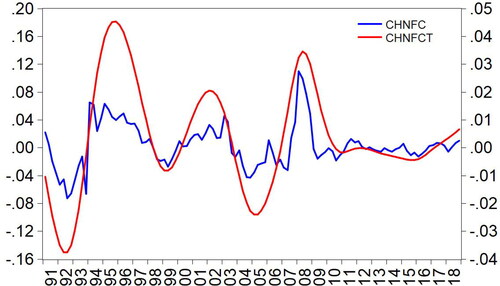
Table 2. Characteristics of China’s financial cycles.

	Phase	Start	End	Duration	Start	End	Amplitude
1	Recession	1991Q1	1992Q3	6	−0.010	−0.038	0.027
2	Expansion	1992Q3	1995Q4	13	−0.038	0.045	0.083
3	Recession	1995Q4	1999Q2	14	0.045	−0.008	0.054
4	Expansion	1999Q2	2002Q1	11	−0.008	0.021	0.029
5	Recession	2002Q1	2005Q1	12	0.021	−0.024	0.045
6	Expansion	2005Q1	2008Q2	13	−0.024	0.035	0.059
7	Recession	2008Q2	2015Q3	29	0.035	−0.004	0.039
8	Expansion	2015Q3	2018Q4	13	−0.004	0.007	0.011
Average	Expansion			12.5			0.045
	Recession			15.25			0.041

Note: the durations of recession (expansion) are measured from peak to trough (trough to peak). The unit is quarter.

Source: The Authors.

Several interesting facts emerge from Figure 1. First, we find that the duration of China’s financial cycle has periods of between 6 to 10 years. However, the duration is not stable and tends shows a notable increase from the first to the third cycle. The duration of China's financial cycle is easily overlooked in previous literature, and one contribution of our research is to get the duration of China's financial cycle. Second, the peaks and troughs of China's financial cycle are synchronized with the time of the global financial crisis. This finding supports the results of Borio (2014), Hiebert et al. (2018). Third, the amplitude of China’s financial cycle has decreased since 2010. This result is different than what is reported by Drehmann et al. (2012), who found that the length and amplitude of financial cycles in some developed countries have increased significantly in the past three decades. This shows that the financial cycles of emerging economies and developed economies are very likely to have different trends. Thus, the conclusions drawn by Drehmann et al. (2012) do not necessarily apply to emerging market economies. However, Borio (2014) underlines that an amplitude of the financial cycle depends on macroeconomic policy regimes. In the past decade, frequent government interventions in financial markets were accompanied by a smaller amplitude of China’s financial cycle (Wang & Li, 2020). In future research, we can consider the empirical evidence of the relationship between the amplitude of China's financial cycle and government. In addition, China's financial market has been developing rapidly, and there has been no extensive banking crisis on the Chinese mainland.

Since 2015Q3, China has experienced an expansion phase of the financial cycle. In this regard, Table 2 indicates that each expansion of the Chinese financial cycle lasted from 11 to 13 quarters. Our results are similar to those of Li et al. (2021), that is, China’s financial cycle will enter a recession period after 2018. The results of Li et al. (2021) show that China’s credit cycle, housing cycle, and stock market cycle will all decline after 2018. If the duration of a recession in China follows the observed trend, the upcoming recession will look even longer. The last recession (2008Q2-2015Q3) lasted 29 quarters years. For policy makers, they need to monitor financial market volatility to prevent systematic financial risks caused by high leverage and rapid capital flows. To contrast with China’s financial cycle, our study also estimates the financial cycles in the G7 countries.

4.2. Financial cycle spillover index

Before progressing to study financial cycle spillovers, we first test whether the financial cycle variables for China and G7 countries are stationary. To this end, we use the Augmented Dickey-Fuller (ADF) test. Test results are presented in Table 3. For all countries, the ADF test rejects the null hypothesis that the financial cycle series does not possess a unit root even at the one percent level of significance. This result clearly shows that all of the eight financial series are stationary in 1% levels.

Table 3. Unit Root Test – financial cycles of China and the G7 countries.

Augmented Dickey-Fuller test statistic
Country	CHN	CAN	FRA	GER	ITA	JPN	UK	US
t-Statistic	−3.766	−4.082	−6.530	−4.926	−4.152	−4.471	−3.907	−3.926

Note: This table summarizes results of the Augmented Dickey-Fuller (ADF) tests for a unit root for the financial cycle series of China and the G7 countries. The null hypothesis is that the series features a unit root. We do not include a constant term and a trend. The 1%, 5%, and 10% critical value for the ADF test are -2.586, -1.944, and -1.615 for a test equation.

Source: The Authors.

We now explore China’s financial cycle spillover properties. Following the DY methodology, we employ eight financial cycle variables to construct an eight-variate VAR, and to examine the extent to which China’s financial cycle shocks are transmitted to the G7 countries. The lag length for the VAR model presented in Equation (4)(4) $${\mathit{FCI}}_t={\sum }_{k=1}^p{\mathrm{\Phi }}_k{\mathit{FCI}}_{t-k}+{\epsilon }_t$$(4) , is determined using the Akaike Information Criterion (one lag). Building on the estimated VAR, we compute the FCSI as in Equation (9)(9) $$\mathit{directional}\mathrm{}{\mathit{FCSI}}_{i\to }\left(H\right)=\frac{\sum _{j=1\mathrm{}\mathit{and}\mathrm{}j\ne i}^N{\tilde{\theta }}_{ji}\left(H\right)}{\sum _{j=1}^N{\tilde{\theta }}_{ji}\left(H\right)}$$(9) . We then carry out the forecast error variance decomposition, assuming a 20-quarter-ahead forecasting horizon. We distinguish between static and dynamic FCSI from China to the G7 countries. Results for the static FCSI are visualized in Figure 2.

Figure 2. The static financial cycle spillover from China to the G7 countries.

Source: The Authors.

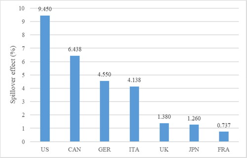
Figure 2 indicates that among the G7 countries, the US appears to be the country that received the most of financial cycle spillovers from China (9.45%), followed by Canada (6.438%), Germany (4.55%) and Italy (4.138%). Hypothesis 1 is confirmed. By contrast, the financial cycle spillovers received by UK (1.38%), Japan (1.26%), and France (0.737%) were the lowest. Given the emergence of China as a global force in the world economy and international financial market in recent decades, a slowdown or even a decrease in the value of financial investments, as well as an increase in financial market volatility, can trigger spillovers to the G7 countries, which are linked with China via investment and trade flows. Our results seem to suggest that financial market volatility in the US could be associated with the disorderly developments in the economy and financial markets in China. Specifically, the VIX volatility index peaked in August 2015, when China’s stock market prices fell sharply despite official support, and the RMB fixing mechanism was adjusted, leading to a RMB depreciation. Therefore, the RMB/USD exchange rate is one of the channels, through which shocks to China’s financial cycle are transmitted to the US. Further, Cashin et al. (2017) suggest that any economic slowdown in China might trigger global spillovers, especially through trade channels. By contrast, the weaker financial cycle spillovers to France, Japan, and the UK are likely to reflect weaker financial links with China. Thus, financial market jitters in China should are a less important source of risk of financial investments in France, Japan and the UK.

On general principles, it is not surprising to observe a small albeit non-trivial (though smaller) financial cycle spillovers from China to developed countries. The average financial cycle spillover effect of China on the G7 countries is 3.993, indicating that China’s financial cycle will have an effect on developed countries. It should be recognized that China is still a net recipient of risks that emerge in international financial markets. However, if China’s transition to the new growth model coincides with the materialization of risks in China’s financial system, it has the potential to generate even larger global financial cycle spillovers (Cashin et al., 2017).

In summary, this discussion shed light on several critical characteristics of China’s financial cycle spillovers. Indeed, international financial and trade links can manifest in larger directional spillovers. Consistently with the findings of majority of previous studies (e.g., Kim et al., 2011; Tsai, 2017), we find that the growing influence of China and the globalization of its financial markets are making fundamental changes to the nature of macroeconomic interdependence and financial markets spillovers between China and the G7 countries.

4.3. Dynamic financial cycle spillover index

Admittedly, while Figure 2 is indicative of the average strength of (static) financial cycle spillovers, it may underestimate their degree and time variation during and after certain events, and overestimate at any other times. However, a fixed-parameter framework is likely to miss potentially important secular and cyclical movements in China’s financial cycle spillovers, and thus it may not to provide a fair representation of the dynamic and volatile nature of China’s financial markets. Therefore, to gain further insights into our empirical analysis, we also generate dynamic financial cycle spillovers. To this end, we undertake a rolling-window estimation of the VAR model of order 1 and we perform a 20-quarter ahead forecast error variance decomposition. Specifically, we use a 24-quarter rolling window to examine the time-varying behavior of the financial cycle spillovers. China’s net financial cycle spillover index is depicted in Figure 3.

Figure 3. Financial cycle net spillovers from China to the G7 countries. Note: Shading denotes the financial crisis as defined by the NBER.

Source: The Authors.

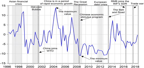
The index takes on positive values in periods, in which China is a net transmitter of spillovers, and it takes on negative values in periods, where China is a net recipient of spillovers. It is evidence that the net financial cycle spillover index underwent significant variation over time and showed some event dependency (Hypothesis 2). During certain periods, the spillover increases to as much as 13.868 (2004Q4) or decreases to as low as −11.013 (2009Q1). The general picture that emerges from Figure 3 is that China was on average a net recipient than a net transmitter of the financial cycle spillovers. In terms of the balance of financial spillovers, the sample period (1996Q4 to 2018Q4) can be divided into four phases.

During the first phase (1996Q4-2000Q1), China’s financial cycle net spillover index shows high instability. Before the 1997-1998 Asian financial crisis, China financial markets generally did not respond to global financial shocks and had only limited on other countries. In mid-1999, China’s net financial cycle spillover index fell from 11.896 (1999Q2) to −6.500 (1999Q3), the largest single-quarter drop in the past two decades. Starting at a value slightly above zero in the first phase, China’s net financial cycle net spillover index varied between 11.896 (1999Q2) and −9.988 (2000Q1). It is worth noting that George Soros’ speculative investments in foreign exchange markets caused currency depreciation in Southeast Asian countries. However, the value of RMB was controlled by the government and the currency was not traded on a free market. Notably, China was a net transmitter of spillovers during the Asian financial crisis in 1997-1998. In fact, during this time, the Chinese government was determined to uphold the RMB in order to avoid undermining Hong Kong’s currency system.

During the second phase (2000Q1-2007Q4), China’s financial cycle spillovers are gradually increasing. This phase started with the Doc-com Bubble in 2000, when the net spillover index climbed from −9.988 (2000Q1) to 1.320 (2001Q2). In the second half of 2001, the net spillover index decreased to −2.833 (2001Q4). China became a member of the World Trade Organization (WTO) on 11 December 2001. Its signified China’s deeper integration into the world economy. The effects from China’s financial cycle spillovers are expected to be buoyant not only because China has opened up its economic market gradually, but also because it has become a world economic power. Indeed, China’s GDP was expanding significantly from 2000 to 2007. The emergence of China coincided with the international spillover effects of surges in China’s financial market volatility. It is thus not surprising to observe China’s financial cycle net spillover peaked to 13.868 (2004Q4), the highest value in during the sample period. During this period, China’s stock market experienced significant growth. For example, the CSI 300 index increased by 474%, from 940 at the beginning of 2006 to more than 5400 in June 2007.

In the third phase (2007Q4-2013Q3), China’s financial cycle net spillovers experienced a prolonged decline. In this phase, the value of China’s financial cycle net spillover index fell to −11.013 in 2009Q1, the lowest value over the sample period, which is associated with the 2007 US subprime mortgage crisis and the 2008 global financial crisis. During the crisis, China's financial market was hit by international capital flows and financial market fluctuations. Therefore, the Chinese financial crisis has received a large number of spillover effects from the financial cycles of the G7 countries. The observed pattern in the financial cycle net spillover is consistent with evidence of transmission of information about the 2008 global financial crisis between the financial cycles (Borio et al., 2018), wherein China’s financial cycle is identified as the net recipient of spillover. To mitigate the adverse effects of the 2008 global financial crisis, China’s government announced a 2008-2009 economic stimulus plan for the amount of RMB 4 trillion. At the end of 2008, the Central Bank of China not only lowered the deposit and loan benchmark interest rates five consecutive times, but also lowered the deposit reserve ratio four times. The difficulty of lending to small and medium-sized enterprises in China was also alleviated by the adjustment of monetary policy. Even if this stimulus program had a positive effect on China’s financial markets – when the financial cycle spillover index rebounded to −4.779 in 2009Q4 – China remained the net recipient of financial cycle spillovers. During the period from 2009 to 2010, the spillover experienced episodes of heightened volatility, reaching values close to-5. Consistent with the findings in Chen et al. (2016), emerging economies appeared to recover in 2009 and 2012, but showed signs of overheating in 2010 and 2011. When the European debt crisis unfolded, China’s financial cycle net spillover index continued to decline and fluctuated at low levels.

The fourth phase started in 2013Q4 and ended in 2018Q4, in which the financial cycle net spillover switched from negative to positive values. During this phase, the financial cycle spillover index fluctuated between −5 and 5. After the Belt and Road initiative, also known as the One Belt One Road, was put in operation, the net spillover entered an expansion phase, and took on the value of 7.262 in 2014Q3. However, in 2016Q4, the net spillover dropped back to −7.210, the minimum value in the fourth phase. Following the internationalization of the RMB, the IMF has added the RMB to the basket of special drawing rights (SDR) since October 2016. In 2016 and 2017, the net spillover fluctuated slightly between −3 and −4. In 2018, the President Trump’s administration-imposed import tariffs on approximately $283 billion of US imports, with rates ranging between 10% and 50%. In response, the US trading partners, especially China, retaliated with tariffs averaging 16% on approximately $121 billion of US exports. We argue that, while the developed countries have strong monetary policy and sound financial markets, they cannot fully isolate a country from the effects of a sharp increase in China’s financial market volatility. Furthermore, the financial cycle net spillover has shown a buoyant trend since the trade war.

On balance, China acted more as net a recipient rather than a net transmitter of the financial cycle spillovers (Hypothesis 3). This implies that international capital flows have brought volatility and shocks to the Chinese financial market, such as the Asian financial crisis and the 2008 international financial crisis. The finding suggests China is not considered as a safe haven for the financial markets of the G7 countries. The 2008 global financial crisis resulted in a direct shock that spread to China financial markets rapidly (Kim et al., 2015). More specifically, China was a net transmitter of the financial cycle spillovers in the period before the 2008 global financial crisis, with a special emphasis on 2004-2005 and 2007, when the Chinese economy experienced high rates of growth. The spillover index surged again in 2014-2015, after the Belt and Road initiative was put into operation. By contrast, China acted as a net recipient of spillovers from 1999 to 2003, which coincided with the dot-com bubble and the beginning of the WTO membership of China. It became a net recipient of financial cycle spillovers from 2008 to 2013, which coincided with the global financial crisis and the European sovereign debt crisis. Peaks and troughs in China’s financial cycle net spillover index are synchronized with specific economic events. Such economic events tend to increase the uncertainty in China financial markets, which result in a variation of the spillover (You et al., 2017). China revitalized the economy by adjusting base currency during the constriction, which is reflected in the Quantitative easing (QE) policy formulated by the Chinese government. In the following quarters, the financial cycle spillover index rebounded to a relatively high value. To capture the time variation in China’s financial cycle spillover to different countries, we also examine the directional spillovers of China’s financial cycle to each the G7 countries, which are depicted in Figure 4. They are estimated by the VAR model presented in Equation (7)(7) $${\tilde{\theta }}_{ij}\left(H\right)=\frac{{\theta }_{ij}\left(H\right)}{\sum _{j=1}^N{\theta }_{ij}\left(H\right)}$$(7) with one lag and 20-quarter forecast error variance decompositions estimated using 24-quarter rolling windows. The areas in the plot indicate China’s financial cycle dynamic contributions to the G7 countries.

Figure 4. Financial cycle spillovers from China to each of the G7 countries.

Source: The Authors.

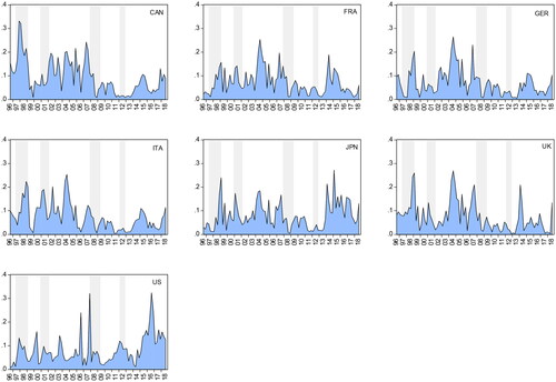
Figure 4 shows variation over time in China’s financial cycle spillover in specific periods. Moreover, the trends of China’s financial cycle spillover to each country is generally consistent with the trend of the index of Figure 3. The directional spillovers also show evidence of heterogeneity across the G7 countries. For instance, a closer look suggests that the direction spillovers take on slightly higher values the US and Canada than to the other G7 countries. Overall, the results echo our conclusions that originated from the analysis of Figure 2. Specifically, the surges of the financial cycle spillover to the US in recent years most likely reflect its cross-country trade links and financial linkages with China.

4.4. Robustness checks

We now turn to examine if our key findings are robust to the rolling window length and the forecast horizon. To this end, we now adopt longer 28-quarter and 32-quarter rolling window lengths (WL), and two different forecast error variance decomposition forecast horizons, with 24-quarter and 28-quarter horizon ($H$). They are used to explore whether the use of alternative $H$-step-ahead forecast error variance decompositions and alternative rolling windows affects the results of China’s financial cycle directional spillovers.

The results appear largely robust to variation in window length and forecast horizon. China’s financial cycle spillover index for the 28-quarter and 32-quarter rolling window appears to be more stable over time. The reason is that it uses more observations but generally has a similar path to the 24-quarter rolling window length. We utilize longer steps (24-quarter and 28-quarter horizon) while holding the rolling window length constant at 24-quarter. The results remain qualitatively similar. It is worth noting that China’s financial cycle variance spillover index matrix may change if the forecast horizon ($H$) is set to be too small. The matrix, however, converges quickly to a stable value when $H$ goes higher.

5. Conclusion

This study highlights and empirically analyzes the financial cycle spillover from China to the G7 countries. We utilize a state-space model to measure the financial cycles of China’s and the G7 countries at first. Subsequently, we employ the spillover index proposed by Diebold and Yilmaz (2012) to examine the static and dynamic financial cycle spillover from China to the G7 countries over the period 1990Q1 to 2018Q4.

We find several core stylized features while characterizing China’s financial cycle. The frequency of China’s financial cycle has periods of between 6 to 10 years and tends to become lower. Furthermore, the peaks and troughs of China's financial cycle are synchronized with the time of the global financial crisis. This finding supports the results of Borio (2014), Hiebert et al. (2018). Finally, the amplitude of China’s financial cycle has decreased since 2010. The corollary of this result is that the government frequent intervention in financial markets has been accompanied by a smaller amplitude of China’s financial cycle in the past decade. Furthermore, China’s financial market is expanding more robustly than we anticipate.

This paper also shows that China plays the role of a net recipient most of the time. Since 2000, China’s financial cycle has received volatility spillovers from the financial cycles of G7 countries, except for the periods of 2004-2005 and 2014-2015. China's financial cycle net spillover index fluctuates widely and is vulnerable to economic events such as the financial crisis. This implies that international capital flows have brought volatility and shocks to the Chinese financial market, such as the Asian financial crisis and the 2008 international financial crisis. China urgently needs monitor financial market volatility to prevent systematic financial risks caused by high leverage and rapid capital flows. From China's financial cycle spillover trend, the financial cycle response to information can be extracted to help policymakers predict the trend, facilitating their formulation of financial strategy. In addition, during 2004-2005 and 2014-2015, the G7 countries also suffered from financial cycle spillovers from China. The US received the most of the financial cycle spillovers from China, followed by Canada, Germany, and Italy. The amount of the financial cycle spillover from China to the US most likely reflects its cross-country trade links and financial linkages with China. This finding also conveys an important message to the financial markets in developed countries. The widely-accepted belief that the emergence of China brings about the international spillover effects of surges in China’s financial market volatility. China’s financial cycle spillovers are becoming more diversified and related to more market linkages. Consisting with the findings of the majority of previous studies (e.g., Kim et al., 2011; Tsai, 2017), we find that the growing influence of China and the globalization of its financial markets are making fundamental changes to the nature of macroeconomic interdependence and financial markets spillovers between China and developed (G7) countries.

This study can open new avenues for future research. As a first extension, further research may examine the financial cycle spillovers across major emerging market economies (BRICS) along with the developed countries (G7). As a second extension, future research could study the determinants of China’s financial cycle spillovers. On this subject, Cashin et al. (2017) suggest that China’s new growth model has the potential to create even larger global spillovers.

Disclosure statement

No potential conflict of interest was reported by the authors.

References

- Borio, C. (2014). The financial cycle and macroeconomics: What have we learnt? Journal of Banking & Finance, 45, 182–198. https://doi.org/10.1016/j.jbankfin.2013.07.031
- Borio, C. E., Drehmann, M., & Xia, F. D. (2018, December). The Financial Cycle and Recession Risk. BIS Quarterly Review.
- Cashin, P., Mohaddes, K., & Raissi, M. (2017). China's slowdown and global financial market volatility: Is world growth losing out? Emerging Markets Review, 31, 164–175. https://doi.org/10.1016/j.ememar.2017.05.001
- Chen, Q., Filardo, A., He, D., & Zhu, F. (2016). Financial crisis, US unconventional monetary policy and international spillovers. Journal of International Money and Finance, 67, 62–81. https://doi.org/10.1016/j.jimonfin.2015.06.011
- Claessens, S., Kose, M. A., & Terrones, M. E. (2012). How do business and financial cycles interact? Journal of International Economics, 87(1), 178–190. https://doi.org/10.1016/j.jinteco.2011.11.008
- Diebold, F. X., & Yilmaz, K. (2012). Better to give than to receive: Predictive directional measurement of volatility spillovers. International Journal of Forecasting, 28(1), 57–66. https://doi.org/10.1016/j.ijforecast.2011.02.006
- Drehmann, M., Borio, C., & Tsatsaronis, K. (2012). Characterising the financial cycle: Don’t lose sight of the medium term! Working paper [No.380], Bank for International Settlements.
- Ghosh, S. (2020). Asymmetric impact of COVID-19 induced uncertainty on inbound Chinese tourists in Australia: Insights from nonlinear ARDL model. Quantitative Finance and Economics, 4(2), 343–364. https://doi.org/10.3934/QFE.2020016
- Hammoudeh, S., Nguyen, D. K., & Sousa, R. M. (2014). China’s monetary policy and commodity prices. Journal of International Money and Finance, 27, 61–85.
- Hiebert, P., Jaccard, I., & Schüler, Y. (2018). Contrasting financial and business cycles: Stylized facts and candidate explanations. Journal of Financial Stability, 38, 72–80. https://doi.org/10.1016/j.jfs.2018.06.002
- Kim, B. H., Kim, H., & Lee, B. S. (2015). Spillover effects of the US financial crisis on financial markets in emerging Asian countries. International Review of Economics & Finance, 39, 192–210. https://doi.org/10.1016/j.iref.2015.04.005
- Kim, S., Lee, J. W., & Park, C. Y. (2011). Emerging Asia: Decoupling or recoupling. The World Economy, 34(1), 23–53. https://doi.org/10.1111/j.1467-9701.2010.01280.x
- Kolia, D. L., & Papadopoulos, S. (2020). The levels of bank capital, risk and efficiency in the Eurozone and the US in the aftermath of the financial crisis. Quantitative Finance and Economics, 4(1), 66–90. https://doi.org/10.3934/QFE.2020004
- Krishnamurthy, A., & Muir, T. (2017). How credit cycles across a financial crisis (No. w23850). National Bureau of Economic Research.
- Kumhof, M., Rancière, R., & Winant, P. (2015). Inequality, leverage, and crises. American Economic Review, 105(3), 1217–1245. https://doi.org/10.1257/aer.20110683
- Li, T., Zhong, J., & Huang, Z. (2020). Potential dependence of financial cycles between emerging and developed countries: Based on ARIMA-GARCH copula model. Emerging Markets Finance and Trade, 56(6), 1237–1250. https://doi.org/10.1080/1540496X.2019.1611559
- Li, X.-L., Yan, J., & Wei, X. (2021). Dynamic connectedness among monetary policy cycle, financial cycle and business cycle in China. Economic Analysis and Policy, 69, 640–652. https://doi.org/10.1016/j.eap.2021.01.014
- Li, Z. H., Dong, H., Huang, Z. H., & Failler, P. (2018). Asymmetric effects on risks of virtual financial assets (VFAs) in different regimes: A case of bitcoin. Quantitative Finance and Economics, 2(4), 860–883. https://doi.org/10.3934/QFE.2018.4.860
- Li, Z., Wang, Y., & Huang, Z. (2020). Risk connectedness heterogeneity in the cryptocurrency markets. Frontiers in Physics, 8, 243. https://doi.org/10.3389/fphy.2020.00243
- Mazur, M., Dang, M., & Vega, M. (2021). COVID-19 and the March 2020 stock market crash. Evidence from S&P1500. Finance Research Letters, 38, 101690. https://doi.org/10.1016/j.frl.2020.101690
- McIver, R. P., & Kang, S. H. (2020). Financial crises and the dynamics of the spillovers between the US and BRICS stock markets. Research in International Business and Finance, 54, 101276. https://doi.org/10.1016/j.ribaf.2020.101276
- Miranda-Agrippino, S., & Rey, H. (2020). US monetary policy and the global financial cycle. The Review of Economic Studies, 87(6), 2754–2776. https://doi.org/10.1093/restud/rdaa019
- Ng, T. (2011, June). The predictive content of financial cycle measures for output fluctuations. BIS Quarterly Review.
- Rey, H. (2015, March). Dilemma not trilemma: The global financial cycle and monetary policy independence. Working paper [No. w21162]. National Bureau of Economic Research.
- Schularick, M., & Taylor, A. M. (2012). Credit booms gone bust: Monetary policy, leverage cycles and financial crises, 1870–2008. American Economic Review, 102(2), 1029–1061. https://doi.org/10.1257/aer.102.2.1029
- Schüler, Y. S., Hiebert, P., & Peltonen, T. A. (2015). Characterising the financial cycle: A multivariate and time-varying approach. Working paper [No. 1846], European Central Bank.
- Schüler, Y. S., Hiebert, P., & Peltonen, T. A. (2017). Coherent financial cycles for G-7 countries: Why extending credit can be an asset. Working paper [No. 43], European Systemic Risk Board.
- Shen, H., Tang, Y., Xing, Y., & Ng, P. (2021). Examining the evidence of risk spillovers between Shanghai and London non-ferrous futures markets: A dynamic Copula-CoVaR approach. International Journal of Emerging Markets, 16(5), 929–945. https://doi.org/10.1108/IJOEM-04-2020-0355
- Strohsal, T., Proaño, C. R., & Wolters, J. (2019). Characterizing the financial cycle: Evidence from a frequency domain analysis. Journal of Banking & Finance, 106, 568–591. https://doi.org/10.1016/j.jbankfin.2019.06.010
- Sukharev, O. S. (2020). Economic crisis as a consequence COVID-19 virus attack: Risk and damage assessment. Quantitative Finance and Economics, 4(2), 274–293.
- Tsai, I. C. (2017). The source of global stock market risk: A viewpoint of economic policy uncertainty. Economic Modelling, 60, 122–131. https://doi.org/10.1016/j.econmod.2016.09.002
- Uddin, M. A., Hoque, M. E., & Ali, M. H. (2020). International economic policy uncertainty and stock market returns of Bangladesh: Evidence from linear and nonlinear model. Quantitative Finance and Economics, 4(2), 236–251.
- Wang, B., & Li, H. (2020). The time-varying characteristics of the Chinese financial cycle and impact from the United States. Applied Economics, 52(11), 1200–1218. https://doi.org/10.1080/00036846.2019.1659500
- Wang, Z., Li, Y., & He, F. (2020). Asymmetric volatility spillovers between economic policy uncertainty and stock markets: Evidence from China. Research in International Business and Finance, 53, 101233. https://doi.org/10.1016/j.ribaf.2020.101233
- Wei, Z., Luo, Y., Huang, Z., & Guo, K. (2020). Spillover effects of RMB exchange rate among B&R countries: Before and during COVID-19 event. Finance Research Letters, 37, 101782.
- Xu, W., Ma, F., Chen, W., & Zhang, B. (2019). Asymmetric volatility spillovers between oil and stock markets: Evidence from China and the United States. Energy Economics, 80, 310–320. https://doi.org/10.1016/j.eneco.2019.01.014
- You, W., Guo, Y., Zhu, H., & Tang, Y. (2017). Oil price shocks, economic policy uncertainty and industry stock returns in China: Asymmetric effects with quantile regression. Energy Economics, 68, 1–18. https://doi.org/10.1016/j.eneco.2017.09.007