Stock market prediction using weighted inter-transaction class association rule mining and evolutionary algorithm

Abstract

Evolutionary computation and data mining are two fascinating fields that have attracted many researchers. This paper proposes a new rule mining method, named genetic network programming (GNP), to solve the prediction problem using the evolutionary algorithm. Compared with the conventional association rule methods that do not consider the weight factor, the proposed algorithm provides many advantages in financial prediction, since it can discover relationships among the attributes of different transactions. Experimental results on data from the New York Exchange Market show that the new method outperforms other conventional models in terms of both accuracy and profitability, and the proposed method can establish more important and accurate rules than the conventional methods. The results confirmed the effectiveness of the proposed data mining method in financial prediction.

Keywords:

• Evolutionary computations
• decision analysis
• association rule mining
• genetic network programming
• stock movement prediction

JEL CODES:

• C40
• C45
• C53

1. Introduction

Stock market prediction has always been an intriguing issue in research and a great challenge because of the complex and volatile nature of the problem. Because the accurate prediction of stock movement may attract large profits in trading, many technologies have been applied to this field. Existing techniques for stock market prediction can be separated into three categories: fundamental analysis, technical analysis, and technological methods. Technological methods rely on the use of mathematical models and computer techniques to search for the optimal investment strategy through simulations. Artificial neural networks, genetic algorithms, genetic programming, support vector machines, and data mining are the most common methods used for these predictions (Chandar, 2021; Chen et al., 2021; Ding et al., 2020; Kim & Sohn, 2010; Sermpinis et al., 2013; Trippi & Turban, 1992; Y. Wang et al., 2021; Wong et al., 2010; Yang et al., 2002). However, most of these methods focus on the stock price, disregarding a large amount of useful information that exists among different stocks. In an attempt to overcome this problem, the weighted inter-transaction class association rule (WICAR) is proposed in this paper to represent the relationships among attributes from different transactions, which has proven to be quite useful in terms of stock market prediction.

In the era of big data, it is imperative to extract effective information from massive amounts of data, and to explore the underlying rules between various structured data and unstructured data, so as to better serve forecasting and decision-making. As one of the optimization algorithms in the field of machine learning, evolutionary computing has shown clear advantages in previous research and practice. Therefore, this study further explores the application of evolutionary computing in the financial field. In this research, WICAR and GNP are used to predict the movement of stock prices to make an investment decision accordingly. The paper contributes to the computing and finance literature in several ways. First, a rule mining algorithm based on GNP is designed to find the inter-transaction association rules, which are regarded as an approximate solution. In comparison with the Apriori algorithm, which is an accurate approach, the approximate solution is more suitable for a large-scale database. Second, the concept of weights is used to identify the rules that are more important or reliable. As the importance of each association rule is different, more effective rules can be determined by considering the weights. Third, the relationship between the trading volume and stock prices utilized in weighted association rule mining is combined with the basic idea of deciding the weight according to the variation in the trading volume. In particular, a novel contribution of the WICAR method is that it is a dynamic weighting algorithm. This is of special importance because in time series data, the weight of each transaction item cannot be fixed. It should be emphasized that the proposed evolutionary-based method can be used not only in the financial market, but also in many other fields, such as for an elevator group supervisory control system, a bidding strategy consisting of multiple rounds in an English auction, an intrusion detection system for the internet, and a traffic prediction system.

The remainder of this paper is organized as follows. In Sec. 2, background information and a literature review are provided. In Sec. 3, the structure of the model is described. In Sec. 4, the weighted association rule mining method based on a GNP structure is explained. In Sec. 5, the experimental environment, conditions, and results are presented. Finally, Sec. 6 concludes the paper.

2. Literature review

In recent decades, data mining has been a powerful new technology in the field of artificial intelligence with great potential to focus on the most important information in the data. Data mining can be considered as an ingredient of knowledge discovery in database (KDD), which has attracted the interest of many researchers. Several data mining methods, such as classification methods, association rules mining, and cluster analysis have been proposed and widely used in various fields (Cassioli et al., 2013; Cheng & Cheng, 2019; Corne et al., 2012; De Angelis & Dias, 2014; Han & Kamber, 2006; Kanungsukkasem & Leelanupab, 2019; Wang et al., 2012, 2017, 2019).

In the field of data mining, association rules mining is a useful method for discovering the interesting relationships hidden within a large-scale database. Association rules mining was proposed in the early 1990s (Agrawal et al., 1993). The basic idea of this method is to identify items that frequently appear concurrently. These frequent item sets, which comprise an antecedent part (X) and a consequent part (Y), can be considered as rules or patterns (X → Y). A well-known algorithm for mining the association rules is the Apriori algorithm (Agrawal & Srikant, 1994). This algorithm provides accurate results by resorting to the support-confidence framework to identify frequent item sets that exceed the given minimum support and confidence threshold. More specifically, the Apriori algorithm is an algorithm that finds frequent itemsets and generates association rules based on them. Its essence is an iterative method of layer-by-layer search, and each search is divided into two stages: generating candidate sets and testing support. This algorithm is easy to understand and easy to implement, and is one of the classic algorithms in the field of data mining. Subsequently, many other algorithms have been proposed with the aim of increasing the efficiency of the association rules. Four methods are usually used to reduce the computational cost: reducing the number of passes through the database (Agarwal et al., 2001; Yuan & Huang, 2005), sampling the database (Chuang et al., 2005; Li & Gopalan, 2005), adding additional constraints to the structure of patterns (Manning & Keane, 2001; Parthasarathy et al., 2001), or using parallelization (Do et al., 2003; Gebali et al., 2019; Hou et al., 2018; Wojciechowski & Zakrzewicz, 2002).

In addition to association rules which provide accurate solutions, heuristics and genetic solutions have also been proposed for large-scale databases. Ashish and Bhabesh used a Pareto-based genetic algorithm to extract useful and interesting rules (Ghosh & Nath, 2004). Ishida et al. used the greedy randomized adaptive search procedure with path-relinking to recreate rules (Ishida et al., 2009). Shimada and Hirasawa developed mining methods based on genetic network programming (Shimada et al., 2006). The advantages of these delicately designed algorithms are that they are less time-consuming and yield stronger relationship rules. In the analysis of the association rules, favorite measurements of interest are support and confidence. Other measurements have also been studied in relation to association rules (Chan, 2020; Chen et al., 2008; Chen & Shi, 2016; Geng & Hamilton, 2006; Jaggi et al., 2021; Lenca et al., 2008; Long et al., 2020; Menaga & Saravanan, 2021; Su et al., 2019; Sun & Meinl, 2012).

The basic principle of the association rules has been extended to develop more advanced rules, such as, inter-transaction association rule mining, which is an extension of classical association rule mining (Hongjun & Ling, 2000; Tung et al., 2003). This new method is fundamentally different from the initial method because it considers the association rules between different transactions, thus facilitating the application of these rules to the prediction problem. These inter-transaction association rules have been used to predict stock movement (Lu et al., 1998). Yang et al. applied GNP to the inter-transaction association rule mining method to determine the operation strategy in the stock market. Both binary and fuzzy implementations of the method have been introduced (Yang et al., 2011a, 2011b). Although prediction of the stock market aims for high accuracy as well as large profits, researchers mostly focus on the profitability rather than accuracy. However, Yang et al. strived to balance accuracy and profitability, and finally obtained an optimized strategy.

Classical association rule mining does not consider the importance of different rules. Even though different items affect profitability differently, the classical association rule mining method treats all rules equally. Thus, the weighted association rule was proposed to address this shortcoming. The weighted association rule mining method allocates higher weights to the rules that are more interesting to the researchers. In studies of weighted association rule mining, different algorithms have been proposed with different understandings of the ‘weight’ concept. For instance, Wang et al. considered the numerical attributes of an item (Wang et al., 2000). They pointed out that, even though the transactions contain the same items, they are actually different because of the numerical attributes. Another viewpoint of the weighted association rule problem is that different rules are of differing importance to researchers (Tao et al., 2003). Although certain rules have lower criteria of support or confidence, they may be more valuable than those with higher criteria. A weighting method for association rules without pre-assigning weights was also proposed (Sun & Bai, 2008). The method differs from previous ones in that the author introduced w-support under the assumption that good transactions consist of good items. Based on this idea, the weights do not have to be assigned initially.

In addition to the rules discussed above, association rules are very popular and have been applied to marketing, finance, medical sciences, etc. In marketing, mining with the aid of association rules is often used to identify patterns among shopping items, or the relationship/preference between customers and items. The association rule mining method was used to discover the online shopping patterns across websites (Yang et al., 2013). An advertising algorithm was developed to choose potential customers for new products based on the association rules (Hwang & Yang, 2008). In the financial field, mining based on association rules is often used for credit card analysis, such as detecting the fraudulent use of these cards (Sánchez et al., 2009; Song et al., 2021; L. Wang et al., 2021; Yao, Cai, and Wang, 2021).

The focus of this study is genetic network programming (GNP), which plays a key role in the proposed algorithm. GNP can be considered a natural extension of the genetic algorithm (GA) and genetic programming (GP), and it uses an iterative process to reach the optimal solution. GNP was proposed to solve more complicated problems, and it has already been identified as an effective method for solving dynamic problems (Mabu et al., 2007). In particular, GNP was employed in the estimation of distribution algorithms to predict traffic conditions (Li et al., 2010). GNP was also used to solve the problem presented by the elevator group supervisory control system (Hirasawa et al., 2008). Additional details of GNP are provided in Sec. 3.

In capital markets, the trading volume is the number of shares or contracts traded in the security market during a given period of time. This information is important for investors in predicting the movement of stocks. Many studies have focused on the relationship between trading volumes and stock prices. Studies show that volume fluctuations are accompanied by the appearance of new information. The different views of investors, the different expectations for the price of a stock can lead to a great exchange among shareholders. The relationship between volumes and prices has already been examined by a statistical method (Ying, 1966), the main conclusions of which were subsequently summarized (Sun, 2003), and can be listed as follows:

• A small volume is usually accompanied by a fall in price.

• A large volume is usually accompanied by a rise in price.

• A large increase in volume is usually accompanied by a large price change.

• A decrease/increase in the volume for five straight trading days is expected to cause the price to fall/rise over the next four trading days.

Other views also exist in the literature. Certain scholars consider the volume to be positively correlated with an absolute price change (Karpoff, 1987), whereas others consider the trading volume to be heavy during a bull market, but light during a bear market (Epps, 1975, 1977). Previous research on association rule mining did not consider the impact of the trading volume on stock movement. This has prompted the current study, which uses the relationship between these two factors, to improve the association rule mining method.

3. Model description

3.1. GNP structure

Genetic network programming, GNP, has a graph structure which consists of three types of nodes: a start node, judgment nodes, and processing nodes, as displayed in Figure 1(a). These three types of nodes connect to each other with directions. A connection is randomly generated during the initialization of GNP individuals. The start node is the starting point of an individual. The judgment nodes operate as IF-THEN type logical functions to determine the next node depending on the current information, and these nodes form a set J₁, J₂, …, J_m. The processing nodes are used to execute decisions and are denoted by P₁, P₂, …, P_n. These decisions are buying and selling actions, which are determined by thresholds and the values of the variables.

Figure 1. Structures of GNP individual and GNP node.

Source: drawn by authors with the help of R software.

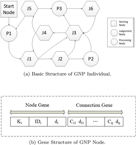
The gene structure of one GNP node is displayed in Figure 1(b). Each node has two segments: the node gene and connection gene. The node gene indicates the node type, node ID, and time delays. The connection gene indicates the connections to other nodes. The node gene K_i indicates the type of node i, where 0 represents the starting node, 1 the judgment node, and 2 the processing node. The ID_i is the identification of the node and d_i signifies the time delays. In this study, time delay is defined as the width of a sliding window used to determine the inter-transaction association rules. The connection gene defines the connection of node i to other judgment and processing nodes. For example, $C_{i1}$ refers to the node in the first branch of node i, and $d_{i1}$ indicates the time delay from node i to the node in the first branch of node i. Based on this structure, GNP employs genetic operators of selection, i.e., crossover and mutation, which are the same in a genetic algorithm.

3.2. Data structure

The data structure determines the mining method. In this research, two basic databases were used for association rule mining. The first is the transactional database, the rows of which contain the transaction records. The second is the weight database, which contains the weights of each transaction. In Table 1, the columns are the attributes denoted as A₁, A₂ and A₃, which are part of the transaction captured from the transaction database.

Table 1. Price return of transaction.

T	A1	A2	A3	C
1	0.02	−0.02	0.05	0.01
2	0.03	0.03	−0.05	−0.02
3	0.00	−0.02	−0.06	0.00
4	0.04	0.05	0.01	0.03
5	−0.02	−0.04	−0.03	0.01

Source: calculated by authors via R software.

Application of the association rule to discrete data requires that the transaction data be discretized, to obtain the database presented in Table 2. If the attribute value is larger than zero, the discrete result is (1,0,0). If the attribute value is equal to zero, the discrete result is (0,1,0), and if the attribute value is less than zero, the discrete result is (0,0,1). After this discretized transaction, the number of attributes in the previous database is multiplied by 3 for the new attributes in the transaction database. In this example, the three attributes become nine attributes after discretization, which means that the attributes of A₁, A₂, A₃ become $A_1^{Up},A_1^{\mathit{Stay}},A_1^{\mathit{Down}},\dots ,A_3^{Up},A_3^{\mathit{Stay}}$ and $A_3^{Down}.$

Table 2. Database after transformation.

T	A1			A2			A3			C
	Up	Stay	Down	Up	Stay	Down	Up	Stay	Down
1	1	0	0	0	0	1	1	0	0	2
2	1	0	0	1	0	0	0	0	1	0
3	0	1	0	0	0	1	0	0	1	1
4	1	0	0	1	0	0	1	0	0	2
5	0	0	1	0	0	1	0	0	1	2

Source: calculated by authors via R software.

The class data in the consequent part of the association rules include the class information, as listed in the rightmost column of Table 2 and denoted by the variable C. In this research, C pertains to stock prediction and represents the stock movement to predict for the next day. The class data are discretized into three categories, i.e., the Up, Stay, and Down categories, which are indicated by 0, 1, and 2, respectively. If the original class data are larger than zero, they are coded as 2. If the class data are equal to zero, they are coded as 1, and if they are less than zero, they are coded as 0.

Table 3 is an example of the weight database of the transaction. The fact that the weight database resembles the transaction database is easily recognized. The attribute value of each transaction has a weight value associated with it, but the class data are not assigned weights. This is the difference between the data structures of the transactional and weight databases.

Table 3. Example of the weight database of a transaction.

T	A1	A2	A3
1	1.1	0.9	1.2
2	0.7	1.0	1.3
3	0.8	1.1	1.5
4	0.9	1.4	0.8
5	0.9	1.2	1.3

Source: calculated by authors via R software.

3.3. Weighted inter-transaction class association rule

As mentioned in the literature, the weighted association rule is an improvement over the classical association rule used for mining. The weighted association rule prioritizes the rules by way of weights to modify the results obtained with association rule mining. The main objective of this method is to use the weight of each item/attribute to recalculate the criteria of the association rule.

3.3.1. Definitions in the weighted association rule

• Weight of Item

  In the database discussed above, an attribute in a transaction is known as an item¹, which is the minimum unit in the database. An item can be considered as a product purchased during shopping. In the prediction of stock movement, an item is the variation of stock prices, whereas the weight of the item is the importance of the item. Most of the time, the weight needs to be decided by researchers before the mining process starts.

• Weight of Itemset.

  The itemset is the combination of items. The weight of the itemset is the average weight of the items in the itemset and is calculated by the following formula: (1) $$\mathit{weight}(\mathit{itemset}(k))=\frac{\sum _{i=1}^{n}we\mathit{ight}(\mathit{item}(i))}{n},$$(1) where n is the number of items in itemset k. The combination of all the itemsets forms the universal itemset.

• Weight of Transaction.

  A transaction can be thought of as a subset of the universal itemset. In other words, a transaction is an itemset extracted from the universe. Therefore, the method used to calculate the weight of a transaction is the same as that used to obtain the weight of an itemset. The weight of the transaction can be calculated as follows: (2) $$\mathit{weight}(t_i)=\frac{\sum _{k=1}^{m}we\mathit{ight}(\mathit{item}(k))}{m},$$(2) where $\mathit{weight}(\mathit{item}(k))$ is the weight of item k, and m is the number of items in transaction t_i. Therefore, the weight of a transaction can be thought of as representing the average value of the stocks in the transaction.

• Weighted Support.

  The support value is one of the most popular measures in association rule theory. It indicates the frequency of the transaction in the entire database, with a larger frequency indicating a more useful transaction. After the weight has been determined, the support can be modified by the weight. In classical association rule mining, the association rule is supposed to be $A\Rightarrow B,$ where A and B are itemsets. The extent to which this association rule is supported is the proportion of transactions that contain A and B at the same time. That is (3) $$\begin{array}{cccc}\mathit{support}(A\Rightarrow B)\hfill & =P(A\cup B)\hfill & =\frac{\#\text{transaction}(A\cup B)}{\#\text{total transactoin}}\hfill & =\frac{\sum _{t=1}^{n}I(t)}{n},\hfill \end{array}$$(3) where t is the transaction, and I(t) is an indicator function, i.e., (4) $$I(t)=\{\begin{array}{cc}1\hfill & \text{if\hspace{0.5em}A\hspace{0.5em}and\hspace{0.5em}B\hspace{0.5em}appear}\hfill \\ 0\hfill & \text{otherwise}\hfill \end{array}$$(4) Each time A and B appear in one transaction, the numerator adds one. Therefore, the weight of each item is the same as in conventional methods. Introduction of the weight into the support function modifies the function as follows. (5) $$\mathit{weighted}\mathit{support}(A\Rightarrow B)=\frac{\sum _{t=1}^{n}we\mathit{ight}(t)I(t)}{\sum _{t=1}^{n}we\mathit{ight}(t)},$$(5) where weight(t) is the weight of transaction t, and n is the number of transactions.

  This modified support function considers the weight of the transactions, which means that for each transaction the weight of the transaction is added to the numerator. Therefore, transactions with more weight are assigned higher support criteria even if they appear infrequently.

  The weighted confidence can be modified in the same way as the support. The confidence measures the probability of itemset B when itemset A appears. (6) $$\text{confidence}(A\Rightarrow B)=P(B|A)=\frac{P(A\cup B)}{P(A)},$$(6) The fact that the numerator does not represent support can easily be demonstrated, while the denominator is the probability that itemset A appears. Therefore, the weighted confidence can be modified as follows: (7) $$\begin{array}{ccc}\text{weighted\hspace{0.5em}confidence}\hfill & =\frac{\mathit{wsp}(A\Rightarrow B)}{\mathit{wsp}(A)}\hfill & =\frac{\sum _{t=1}^{n}we\mathit{ight}(t)I(t)}{\sum _{t=1}^{n}we\mathit{ight}(t)I\prime (t)},\hfill \end{array}$$(7) where wsp represents the weighted support and $I\prime (t)$ is an indicator function, i.e., (8) $$I\prime (t)=\{\begin{array}{cc}1\hfill & \text{if\hspace{0.5em}A\hspace{0.5em}appears}\hfill \\ 0\hfill & \text{else}\hfill \end{array}$$(8)

3.3.2. Dynamic weights of the association rule

In general, determining the weight of each item is a difficult task for at least two reasons. First, the database usually contains hundreds of items, and it is impossible to allocate weights to each itemset. Second, the weight of an itemset is also difficult to decide. Manual allocation, usually makes this a challenging task, especially when the database contains hundreds of items, the task becomes manually insurmountable. A method was proposed to find association rules without pre-assigned weights Sun and Bai (2008), taking into consideration the quality of the transactions using linked-based models.

In this research, a new method was proposed to allocate weights to the items in association rule mining. Existing weighting methods enhance the effects of items that are important, and lessen the effects of those that are unimportant. This means that the relationship between the items and the target variable has to be determined. For example, in the supermarket, the sales profit is strongly related to the sales volume of products. Thus, the regression of the profits on the variables representing the sales volume can be expressed as: (9) $$\begin{array}{cc}\mathit{profit}\hfill & ={\beta }_{1}t\mathit{elevision}+{\beta }_{2}c\mathit{omputer}+\cdots +{\beta }_{n}w\mathit{asher},\hfill \end{array}$$(9) The coefficient of each item is the profit the item contributes or consumes when it increases or decreases by a unit. Therefore, the coefficient can be used as the weight of this item, because the coefficient reflects the importance of the item with respect to the profit, as expressed by the following function: (10) $$\mathit{weight}(\mathit{item}(i))={\beta }_i.$$(10) The weights of the itemset in a transaction can be calculated based on 2, introduced in Sec. 3.3.1.

In certain cases, it is not easy to derive this relationship using regression methods. For example, when predicting stock movement, the objective is to predict the prices of certain specific stocks, and the items in the antecedent are other stocks. The relationship between the target stock and the stocks in the antecedent cannot be determined by a simple regression model. This problem could be solved by finding another variable that has a certain relationship with the target variable and using it as a dummy variable to augment the original one.

Conventional methods assign weights by requiring that the weight of each item be fixed. However, if a dummy variable is used as the weight of an item, the weight does not necessarily always have to be the same. This is referred to as dynamic weighting. For example, because there is a relationship between the stock price movement and the trading volume, and the volume is positively correlated with the absolute price changes, dynamic weighting can provide guidance in determining the weight of the items. In attempting to solve the prediction problem, certain results of previous studies were found to be useful in the discussion on variables or factors having a relationship to stock price movements (Sun, 2003). The author summarized the relationship between the trading volume and stock price as ‘A large increase in volume is usually accompanied by a large price change’. Thus, in the proposed method, the volume fluctuation is used as the weight for the association rule.

Here, the database structure is revisited because the structure determines the weighting method. In the stock price and trading volume database, one row of the database contains the changes in the stock price and the daily trading volumes. Therefore, the approach here is to apply association rule mining to the prediction, and then to use the changes in the stock prices of earlier transactions to predict the stock price changes for the next few days. If the trading volumes are used as the weights, the weights would be different in transactions on different trading days, provided the assumption that trading volumes can be used as weights is correct. Thus, the function of support in weighted association rule mining can be modified as follows:

• Weight of Item.

The weight of an item in different transactions can be denoted as $\mathit{weight}(\mathit{item}(k,i)),$ which indicates the weight of item k in transaction i. Therefore, the difference from the conventional weight is that $\mathit{weight}(\mathit{item}(k,i))$ introduces the dimension of a transaction.

• Weight of Itemset.

The weight of an itemset is modified similar to the weight of an item, in that, the dimension of the transaction is introduced. (11) $$\mathit{weight}(\mathit{itemset}(k,i))=\frac{\sum _{j=1}^{n(k)}we\mathit{ight}(\mathit{item}(j,i))}{n(k)}.$$(11) The weight of itemset k in transaction i, which is the average value of the weights of all items in itemset k in transaction i, and n(k), the number of items in itemset k, are calculated.

• Dynamic Weighted Support of Association Rule

Introducing the dimension of a transaction enables the calculation of the dynamic weighted support of the association rules. In dynamic methods, the dimension does not need to modify the function of support. This is the same for the support function of the weighted association rules because the weight of the itemset already reflects the dimension of the transaction.

4. Inter-transaction association rule mining with GNP

4.1. Rule extraction and criteria calculation

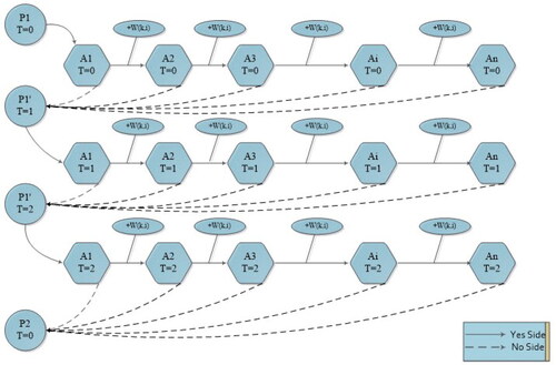
The key aspects of the method extracting the association rule with GNP are the judgment node chain (JNC) and sliding windows (Figure 2). The JNC consists of a series of connected judgment nodes, and the processing nodes are used to select the judgment node to start each association rule. As shown in Figure 2, a JNC has two types of connections: yes-side and no-side. A single JNC is limited in terms of the number of judgment nodes it may contain, which limits the depth of rule in a row. In Figure 2, the maximum number of judgment nodes is n. Similar to other evolutionary algorithms, selection, crossover, and mutation are used for the genetic operators of GNP in association rule mining. The evolution process can be outlined as follows:

Figure 2. Judgment node chains.

Source: drawn by authors with the help of R software.

1. Initialize a randomly generated population.

2. Evaluate the fitness of individuals in the population using a fitness function.

3. Generate new individuals for the next generation by tournament selection and the genetic operations of crossover and mutation.

4. Replace the current population by the new population.

5. If the termination condition is satisfied, then stop; else, go to step (2).

Each JNC represents a transaction, and the judgment nodes are used to determine the attribute that reflects the change of stock prices in the prediction problem. For example, attribute 1 (A₁) denotes the price movement direction of stock 1 in one day, and attribute 2 (A₂) represents that of stock 2 on the same day. To obtain the inter-transaction association rule, another concept, namely that of a sliding window, is introduced. Because several JNCs are combined to present a multi-transaction, the width of the sliding window is the number of combined JNCs. When the window is sliding downwards, a new JNC can be used for association rule mining.

When the judgment node satisfies the condition, the yes-side connection is selected before proceeding to the next judgment node in the same node chain. In the stock prediction problem, the judgment function in the judgment node determines whether the attribute equals 1 or 0. If the condition is not satisfied, the no-side connection is chosen and the function proceeds to the next processing node, which points to the new start judgment node in the next node chain, i.e., the transaction of the following day. Once the search process has been completed, the candidate rule is obtained as follows: (12) $$A_1^0(up)\cap A_2^1(\mathit{down})\cap \dots \cap A_m^w(up)\Rightarrow C(up)$$(12)

The subscript and superscript of the attribute indicate the attribute number and the number of days after the starting day, respectively. Therefore, 12 means that when stock 1 increases on day 0 and stock 2 increases on day 1, …, and stock m increases on day w, it can be predicted that stock C will increase on the next day under the criteria of support and confidence. When the last JNC has been checked, the window slides downward to the next transaction and the same procedure are repeated to determine the next set of candidate rules.

The method for association rule mining is also examined with respect to the database structure. Figure 3 shows a section of the database containing the stock price movements, which also constitutes the sliding window used to search for the candidate rules. The width of the window is 5, with the first four transactions being for the antecedent part of the association rules, and the last transaction for the consequent part of these rules. For example, in Figure 3, after checking that the value of the last attribute is 0, which does not satisfy the condition, the next processing node is selected to proceed to the next transaction.

Figure 3. Rule extraction of the proposed method.

Source: drawn by authors with the help of R software.

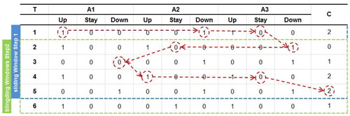
The example displayed in Figure 3 illustrates the methods used in determining a candidate association rule by GNP. The search process starts from the first attribute ($A_1^0(Up)$). Because the value of the attribute is 1, the search moves to the next judgment node in JNC, and the value of the second attribute ($A_2^0(\mathit{Down})$) in the current transaction is also found to be 1. Then, the search moves to the next attribute in the same transaction. Because the value of the third attribute ($A_3^0(\mathit{Stay})$) is 0, the search process in the current transaction is terminated. As suggested by the processing node, attribute 3 in the second transaction ($A_3^2(\mathit{Down})$) is selected. The value of $A_3^2(\mathit{Down})$ is 1, and the search continues with the second transaction. This process continues until the last transaction in the sliding window is completed. The class attribute in the last transaction, that is, the target stock movement in the prediction problem, along with the combination of attributes searched before, establish the following candidate association rule: (13) $$A_1^0(up)\cap A_2^1(\mathit{down})\cap \dots \cap A_m^w(up)\Rightarrow C(up).$$(13)

Then, the sliding window moves downwards by one transaction and restarts the search process, after which the search steps are executed the same way as before. After all the processing nodes have been exhausted, the search process is terminated in this sliding window. Then, the sliding window moves downwards to cover the next transaction, as shown in Figure 3. The search process is executed again in the new sliding window. Because the GNP structure is generated randomly at the beginning, the path from one attribute to another is already set when the GNP is formulated. A large number of GNP individuals and genetic operators guarantee that sufficient association rules are found by using this method. The mined association rule r is stored in the rule pool (RP_k) according to the class of the consequent part of the rule.

During the search process, a counter is used to record the number of items and transactions to calculate the weighted criteria of support and confidence. Because each judgment node has a weight, as shown in Figure 2, the weights are added to the counter each time the judgment node is visited. The counters are described as follows:

Suppose association rule r is $A\Rightarrow C(k),$

• $Ante[A_1][A_2]\dots [A_m]=Ante[A_1][A_2]\dots [A_m]+\frac{1}{m}{\displaystyle \sum _{i=1}^{m}w}eight(A_i),$

where $\mathit{Ante}[A_1][A_2]\dots [A_m]$ is the sum of weights in the antecedent part of the rule and $A_i(i\in \{1,2,\dots m\})$ are the items in the antecedent part (A) of association rule ($A\Rightarrow C(k)$).

• $A{C}_k[A_1][A_2]\dots [A_n]=A{C}_k[A_1][A_2]\dots [A_n]+\frac{1}{n}{\sum }_{i=1}^{n}we\mathit{ight}(A_i),$

where $A{C}_k[A_1][A_2]\dots [A_n]$ is the sum of the weights of class k in rule r.

The use of these counters enables the calculation of the weighted support (wsp) and the weighted confidence (wconf) criteria as follows: (14) $$\mathit{wsp}(r)=\frac{A{C}_k\left[A_1\right]\left[A_2\right]\dots \left[A_n\right]}{\mathit{Ante}\left[0\right]\left[0\right]\dots \left[0\right]-S_{\mathit{max}}(r)},$$(14) (15) $$\mathit{wconf}(r)=\frac{A{C}_k\left[A_1\right]\left[A_2\right]\dots \left[A_n\right]}{\mathit{Ante}\left[A_1\right]\left[A_2\right]\dots \left[A_m\right]},$$(15) where $\mathit{Ante}[0][0]\dots [0]$ is the total number of sliding windows in the database; $S_{\mathit{max}}(r)$ is the maximum interval span over all the attributes in rule r; and $S_{\mathit{max}}(r)$ is used to revise the support in the inter-transaction association rule mining because Ante[0][0]…[0] is not the total number of transactions.

Another criterion, ${\chi }^2,$ is introduced to measure the dependency between the antecedent and consequent in the association rule ($A\Rightarrow B$). The definition of ${\chi }^2$ is as follows: (16) $${\chi }^2(r)=\frac{N\prime {(z\prime -x\prime y\prime )}^2}{x\prime y\prime (1-x\prime )(1-y\prime )},$$(16) where $N\prime$ is the revised number of total transactions, and N is the total number of transactions. (17) $$N\prime =N-S_{\mathit{max}}(A\cup B),$$(17) (18) $$x\prime =\frac{t(A)}{N-S_{\mathit{max}}(A\cup B)},$$(18) (19) $$y\prime =\frac{t(B)}{N-S_{\mathit{max}}(A\cup B)},$$(19) (20) $$z\prime =\frac{t(A\cup B)}{N-S_{\mathit{max}}(A\cup B)},$$(20) where t(X) is the number of transactions that contain itemset X.

4.2. Fitness function and genetic operators

The above-mentioned association rule extraction methods can be used to obtain the candidate rules. However, this is insufficient, because the GNP structure, which is initially formulated randomly, only represents part of the rule space. Based on the fitness function and genetic operators, more effective rules can be obtained. The fitness function is designed as: (21) $$F=\sum _{r\in R}\{{\chi }^2(r)+10(n_{\mathit{ante}}(r)-1)+{\alpha }_{\mathit{new}}(r)\}.$$(21) where ${\chi }^2(r)$ represents the strength of the relationship between the antecedent and consequent in rule r; $n_{\mathit{ante}}(r)$ represents the number of items in the antecedent part of rule r; and ${\alpha }_{new}(r)$ represents the bonus for new rule r. This fitness function indicates that rules with a higher relationship between the antecedent and consequent, or with more antecedent attributes, attain a higher fitness value.

In genetic operations, the rules that are selected should be retained and reproduced to form a new generation. Upon completion of the crossover and mutation operations, the GNP population of the next generation is generated. The definitions of the crossover and mutation operations are given below.

• Crossover: the parent individuals exchange their nodes and connections to form new individuals.

• Mutation: the parent individual changes the functions and connections of the nodes to change the structure of GNP and form a new individual.

4.3. Classifier model

Usually, association rule mining can generate thousands of rules and stores them in rule pools. For example, if there are m classes in the consequent part of the rules, m rule pools can be set up to classify the rules as Pool(i) (i = 1…m), where Rule(i, j) is rule i in pool j.

The next part of the work is conducted to answer two questions: How should these rules be used? When new data d are provided, which rules are supposed to match? Two classifiers are used to solve these problems: the complete matching classifier and the partial matching classifier. These classifiers differ in that the partial matching classifier considers the effect of time, which means that the partial method assumes that the latest data have priority over the earlier data.

First, the complete matching classifier is introduced:

1. To measure the way in which data d match rule r in each rule pool (RP_k), $S_k(d,r)$ is used as a score for each rule r in class k. (22) $$S_k(d,r)=w(r)\times D_k(d,r),$$(22)

where w(r) is the weight of rule r, which can be the confidence, chi-squared value, or Laplace accuracy. $D_k(d,r)$ is the matching degree of rule r in class k with data d. In the complete matching classifier, $D_k(d,r)=1$ if d matches the antecedent of rule r completely, otherwise $D_k(d,r)=0.$

• 2. After obtaining the score of data d, $S_k(d,r),$ for each rule r, the average matching degree $m_k(d)$ is calculated in each rule pool RP_k by (23) $$m_k(d)=\frac{1}{\left|R{P}_k\right|}\times \sum _{r\in R{P}_k}{S}_k(d,r),$$(23)

where $k=1,2,\dots ,c$ and $\left|R{P}_k\right|$ is the number of rules in rule pool RP_k.

• 3. Then, the largest average matching degree $m_k(d)$ is selected from the rule pool. Class k of this rule pool RP_k is the class to which the current data belongs.

As mentioned before, the partial classifier is modified according to the time of data. Therefore, only the first step needs to be modified in the complete matching classifier. The matching degree is modified in the following way: (24) $$D_k(d,r)=\frac{{\displaystyle \sum _{A\in I(k)}\alpha }(A)\times D_k(d,A)}{{\displaystyle \sum _{A\in I(k)}\alpha }(A)},$$(24) where $\alpha (A)$ is used to discount attribute A according to the time period, which has the form of $v^{\left|o\right|-1}$ ($v\in (0,1],$ and $\left|o\right|$ is the relative domain address of the class attribute from A). $D_k(d,r)$ is the matching degree of rule r in class k with data d. I(k) is the set of rules in class k. The following steps in the partial matching classifier are the same as those in the complete matching classifier.

5. Simulation

5.1. Description of simulations

In this section, the details of our study are presented on the profitability and accuracy of this method for weighted association rule mining to solve the stock prediction problem. The simulation was conducted by selecting 30 stocks as targets stocks. These 30 stocks are included in Dow Jones Industrial Average Index. The reason for this selection is to ensure that the target stocks are more representative. The price data on which the simulations are based were collected from April 23, 2015 to March 16, 2019. This period is divided into two parts for training and testing. The training data gathered in the period ranging from April 23, 2015 to February 23, 2018, were used for the mining association rules of two methods. The testing data were collected from February 24, 2018 to February 17, 2019, and were used to evaluate the profitability and accuracy of the mining methods. Individual stock prices from these periods were used for training and testing. This means that each of the stocks was used for mining inter-transaction association rules during the training period. Then, the trading price of this stock was determined in the testing period according to the rules that were mined in the training period.

Apart from the target stocks, the stocks in the antecedent part of the association rule also need to be selected. Considering the feasibility of the calculation, 50 representative stocks were selected from a total of 1692 stocks using clustering and correlation methods. First, all 1692 stocks were separated into 50 groups by clustering methods. Then, a genetic algorithm was used to select one stock from each group. The parameters of the proposed method are listed in Table 4.

Table 4. Parameters of the class association rule mining method.

Parameters		Parameters
Individuals	120	Support	0.03
Processing nodes	10	Confidence	0.7
Judgment nodes	75	Chi-2	3.84
Attributes	150	Objective stocks	30
Generations	1001	Window size	2/3/4

Source: calculated by authors via R software.

According to the classifier model, CL (mode, weight, filter, discount) was used to represent the classifier. Details of the classifiers are provided elsewhere Yang et al. (2011a). The six classifiers listed in Table 5 achieved superior results, and were used to classify the rules in this research.

Table 5. Six kinds of classifiers.

Classifier	Description
$Cl(c,\mathit{lap},\mathit{all},n)$	Complete matching; Laplace weight; All rules; No discount
$Cl(c,\mathit{lap},K_p,n)$	Complete matching; Laplace weight; K percentage rules; No discount
$Cl(p,\mathit{lap},\mathit{all},n)$	Partial matching; Laplace weight; All rules; No discount
$Cl(p,lap,K_p,n)$	Partial matching; Laplace weight; K percentage rules; No discount
$Cl(p,\mathit{lap},\mathit{all},y)$	Partial matching; Laplace weight; All rules; With discount
$Cl(p,\mathit{lap},K_p,y)$	Partial matching; Laplace weight; K percentage rules; With discount

Source: calculated by authors via R software.

5.2. Simulation results

In this experiment, the profitability and accuracy of the prediction between the weighted inter-transaction association rule and the conventional association rule were compared. A benchmark was also added in the form of a buy and hold strategy, according to which a stock is bought at the beginning and held until the end.

5.2.1. Evaluation of profitability

Table 6 presents the average profitability of 30 stocks in the Dow Jones Index using six classifier models. First, the profitability of the buy&hold method and the association rule method was compared. These results demonstrate that the association rule method can help investors obtain higher returns. In the testing period, the buy&hold strategy only yields a return of 11.5%, whereas the weighted and conventional association rule methods both deliver superior performance.

Table 6. Average profits for 30 stocks of the 6 classifier models (%).

	Weighted method			Conventional method			B&H
Symbol (Company)	1day	2days	3days	1day	2days	3days
AXP (American Express Company)	27.9	14.4	12.1	29.9	16.9	12.9	−17.7
BA (Boeing Co)	−0.4	1.5	3.3	3.3	10.4	21.4	2.8
CAT (Caterpillar Inc)	24.3	24.0	15.2	2.3	15.5	3.3	4.0
CSCO (Cisco Systems Inc)	32.1	40.4	35.7	20.7	18.0	17.8	15.2
CVX (Chevron Corp)	2.7	9.1	−5.4	−2.5	6.4	10.7	3.0
DD (E.I. Du Pont De Nemours And Company)	−5.7	6	15.5	0.4	5.6	3.8	−1
DIS (Walt Disney Company)	5.1	3.6	−8.2	1.8	22.7	−4.2	1.2
GE (General Electric Company)	10	5.4	3.3	2.2	4.6	3.3	2.1
GS (Goldman Sachs Group Inc)	−19.9	−2.8	−17.3	−10.9	−14.9	12.9	−22.1
HD (Home Depot)	36.5	40.8	38.5	32.1	35.9	36.9	31.5
IBM (International Business Machines Corp.)	16	27	19.6	20.1	21.8	16.3	27
INTC (Intel Corp)	36.7	43.8	46.1	38.1	39.6	30.3	36.2
JNJ (Johnson & Johnson)	2.9	5	6.9	14.7	5.3	3.7	10.3
JPM (J P Morgan Chase)	−9.6	13.6	7	6.1	2.8	−1.6	−2.5
KO (Coca-Cola Company)	2.7	8.6	8.5	6.2	8.1	9	7.8
MCD (McDonalds Corp.)	36.8	44.3	42.1	32.6	38.2	33.4	30.3
MMM (3 M Company)	7.6	0.9	−0.2	−4.7	−1	−6.4	−2.5
MRK (Merck & Company)	16.7	23.4	15	14.7	5.3	10.8	16.9
MSFT (Microsoft Corp)	30.6	38.1	33.1	26.4	34.7	31.9	28.2
NKE (Nike Inc)	42.4	45.5	45.6	41.9	40.9	44.0	44.4
PFE (Pfizer Inc)	9.9	15.6	7.7	−1.8	−3.9	12.9	7.7
PG (Procter & Gamble Company)	3.8	7.6	3.8	1.1	0.4	6.8	11.2
T (AT&T Inc)	2.9	15.8	8.8	12.3	−0.3	−9.3	5.9
TRV (Travelers Companies Inc)	9.7	10.8	9.5	−1.3	−0.3	−8.2	0.2
UNH (UnitedHealth Group Inc)	32.3	35.4	32.4	29.1	33.0	29.1	27.3
UTX (United Technologies Corp.)	1.4	11.1	0.3	7.9	14.8	0.8	4.0
V (Visa Inc)	61.0	64.2	50.7	62.9	68.4	66.0	62.3
VZ (Verizon Communications Inc)	8.5	14.5	13.1	10.1	12.1	11.2	6.0
WMT (Wal-Mart Stores)	6.6	6	6	2.1	15.2	16.3	3.0
XOM (Exxon Mobil Corp.)	8.4	10.9	10.9	4.9	8.8	2.3	3.0
Average Profits	14.7	19.5	15.3	13.4	15.5	13.9	11.5

Source: calculated by authors via R software.

Second, the profitability of the weighted and conventional methods was compared. In general, the weighted association rule helps investors with their profits. When the association rule method with a 1-day sliding window was used, the weighted method provided an average return of 14.7% in the testing period, while the conventional method achieved a return of 13.4%. The same results were obtained with simulations using sliding windows of 2 and 3 days. A sliding window of 2 days with the weighted association rule method provided investors with an average return of 19.5%, whereas the return was 15.3% for the sliding window of 3 days. In the case of the conventional method for the same period, the average returns were only 15.5% and 13.9% for sliding windows of 2 days and 3 days, respectively. This result can be explained by the volume, which plays an important role here. Positive and negative information can affect the trading volume of the stock market, which could potentially increase to a high level in a short time, the impact of which usually lasts for a while. When the investors in the market reach an agreement on the new price, or when the information has already been interpreted, the volume returns to the normal level after several trading days. This indicates that the weighted association rule with larger sliding windows is superior to the rule with only one window. A comparison of the profits in different sliding windows with the same mining method reveals that the 2-day sliding window is a more effective choice.

Because classifiers can affect the rules, the best classifier was selected for each stock, which means that the selected classifier maximized profit. This can be used to construct a strategy for a particular stock. Table 7 indicates that the best classifier can provide a higher return compared with the buy&hold strategy. Even compared with the average return of all six classifiers, the best classifier can still be more attractive.

Table 7. Max profits for 30 stocks of the 6 classifier models (%).

	Weighted method			Conventional method			B&H
Symbol	1day	2days	3days	1day	2days	3days
AXP (American Express Company)	40.9	19.6	32.2	45.6	25.3	19.5	−17.7
BA (Boeing Co)	5.1	14.0	15.5	13.0	17.0	34.4	2.8
CAT (Caterpillar Inc)	38.1	49.9	62.2	28.5	40.3	16.6	4.0
CSCO (Cisco Systems Inc)	71.6	48.5	70.0	31.2	32.4	22.0	15.2
CVX (Chevron Corp)	13.6	12.8	1.3	1.4	29.9	25.3	3.0
DD (E.I. Du Pont De Nemours And Company)	3.1	14.4	25	16.4	20.1	11.5	−1
DIS (Walt Disney Company)	18.9	19.3	1.8	33	27.6	26.5	1.2
GE (General Electric Company)	15.5	26.4	12.8	10.8	13.7	5.7	2.1
GS (Goldman Sachs Group Inc)	−0.1	19.2	3.2	5.3	1.6	27.9	−22.1
HD (Home Depot)	45.6	54.3	46.7	41.2	49.5	44.3	31.5
IBM (International Business Machines Corp.)	28.9	31.3	25.1	26.7	28.5	26.3	27
INTC (Intel Corp)	45.4	53.5	52.3	44.6	50.0	44.9	36.2
JNJ (Johnson & Johnson)	5.9	6.3	21.8	19.3	8	6.1	10.3
JPM (J P Morgan Chase)	15.8	32.9	17.9	37.4	15.8	9.7	−2.5
KO (Coca-Cola Company)	6.9	17.5	18.6	7.4	11.8	13.2	7.8
MCD (McDonalds Corp.)	41.8	55.1	49.8	41.14	49.2	46.8	30.3
MMM (3 M Company)	12.9	4.7	11.3	7.6	3.2	−2.8	−2.5
MRK (Merck & Company)	20.4	32.7	20.3	20.4	11.4	13.4	16.9
MSFT (Microsoft Corp)	37.7	45.5	47.6	32.4	41.2	48.6	28.2
NKE (Nike Inc)	50.0	52.1	50.4	53.5	57.1	53.4	44.4
PFE (Pfizer Inc)	15.1	30.3	15.7	1.1	0.8	21.2	7.7
PG (Procter & Gamble Company)	12.4	12.7	10.6	2.5	4.4	9.8	11.2
T (AT&T Inc)	19.2	23.8	15.8	30.0	34.1	13.3	5.9
TRV (Travelers Companies Inc)	19.5	21.9	19.9	3.2	3.5	0.2	0.2
UNH (UnitedHealth Group Inc)	44.1	48.1	39.2	34.2	42.6	36.3	27.3
UTX (United Technologies Corp.)	21.9	29.2	9.6	24.3	29.4	15.2	4
V (Visa Inc)	88.9	89.2	60.0	72.3	88.1	75.6	62.3
VZ (Verizon Communications Inc)	18.1	20.7	19.5	17.2	24.5	22.4	6.0
WMT (Wal-Mart Stores)	14.1	9.9	9.9	23.3	16.1	19.3	3
XOM (Exxon Mobil Corp.)	15.3	24.3	24.3	6.4	11.3	5.2	3
Average Profits	26.2	30.7	27.0	24.4	26.3	23.7	11.5

Source: calculated by authors via R software.

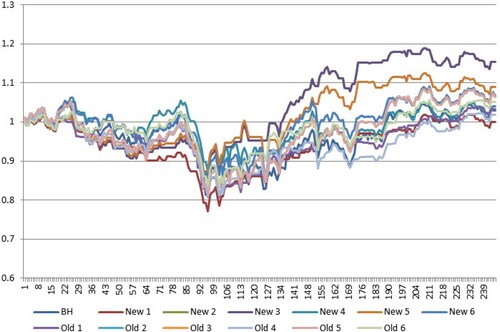
Several stocks were selected to track the profit fluctuations resulting from the association rule methods and the buy&hold strategy.

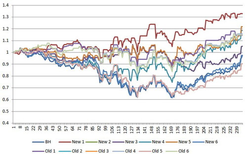
Figure 4 shows the profit fluctuation for Exxon Mobil Corp., with a sliding window of 1 day for each classifier. Note that, at the beginning of the testing period, the results are almost the same for all methods. However, after approximately 3 months, the performance of association rule methods starts to improve. Classifier 3 of the weighted methods performed the best, providing a profit of 15.3%, whereas the buy&hold strategy was less effective and only provided a profit of 3%.

Figure 4. Profit fluctuation for exxon mobil corp.

Source: drawn by authors with the help of R software.

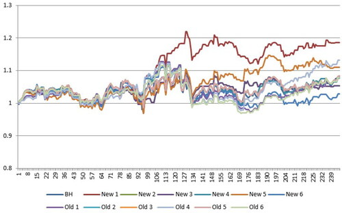
Figure 5 shows the profit fluctuation for J P Morgan Chase & Co, with a sliding window of 2 days. As observed in the chart, classifiers 1 and 5 of the weighted method were effective. Classifier 1 of the weighted method provided a profit of 32.9%. In the case of the buy&hold strategy, a loss of 2.5% of capital was observed.

Figure 5. Profit fluctuation for J.P. Morgan Chase & Co.

Source: drawn by authors with the help of R software.

Figure 6 shows the profit fluctuation for the Coca-Cola company, with a sliding window of 3 days. As shown by the chart, classifiers 1 and 5 of the weighted method delivered good performance, and classifier 1 of the weighted method provided a profit of 18.6%, whereas the profit with the buy&hold strategy was 7.8%.

Figure 6. Profit fluctuation for Coca-Cola Company.

Source: drawn by authors with the help of R software.

Figures 4–6 show that the classifier has a strong impact on the simulation results. A suitable classifier needs to be selected for different stocks. Another point is that the length of the sliding window should suit the prediction problem; a 2-day sliding window performed the best in the simulations.

5.2.2. Ability to attain prediction accuracy

In this study, accuracy is defined as the correct prediction number divided by the total number of records that were tested. As mentioned above, high accuracy does not indicate high profitability. The following cases are examples from a previous study Yang et al. (2011b).

Case 1: The agent correctly predicts the results in four trading days, with each bringing a profit of 1,000 yen, but it fails to predict the result on the fifth trading day, which leads to a large loss of 10,000 yen. In this case, the loss is 6,000 yen and the prediction accuracy is 80%.

Case 2: The agent incorrectly predicts the results in four trading days, with each causing a loss of 1,000 yen, but the prediction is correct on the fifth trading day, which brings a large profit of 10,000 yen. In this case, the profit obtained is 6,000 yen, but the prediction accuracy is 20%.

These two examples clearly indicate that obtaining high profits is of key importance in correctly predicting the stock movement. The association rule, which is weighted by the trading volume, supports this point much more strongly than the conventional method because it assigns higher weights to key transactions. To verify this, the average prediction accuracy was calculated. The results are listed in Table 8.

Table 8. Accuracy of prediction.

	1 day	2 days	3 days
Conventional method	0.460	0.493	0.481
Weighted method	0.494	0.514	0.504

Source: calculated by authors via R software.

These results demonstrate that the weighted method also has an advantage in prediction accuracy compared to the conventional one. The weighted method (with all three sliding windows) is more accurate than the conventional method. Therefore, based on the experimental results in Tables 6 and −7, the proposed weighted method can determine more important and accurate rules than the conventional method, thereby increasing the profits and improving the accuracy.

6. Conclusions and future work

In this paper, a weighted inter-transaction association rule mining method is proposed based on genetic network programming. The idea is that different rules are of different levels of importance to analysts. Rules with larger support and confidence might be less important than rules with little support and confidence, if association rule mining methods are used without considering weights. The weight is determined by analysts depending on the problem. In this research a method was introduced to allocate these weights. The proposed method, which can dynamically assign weights, was applied to the stock market prediction problem to construct trading strategies. To evaluate profitability and accuracy, the mined association rules were used to generate the trading strategy, then the results were compared with those obtained with conventional mining methods. The experimental results demonstrate that the weighted mining method extracts the key rules more effectively than the conventional method, and this characteristic achieves higher prediction accuracy and more profits than the conventional methods.

In the future, a new computational algorithm can be introduced to improve prediction accuracy. First, the trading strategy presented in this paper only includes buying, selling, and holding actions, and the profits are obtained only as a result of an increase in the price of stocks. To solve this problem, the new computational algorithm can introduce a short sales mechanism to imitate the stock market, which is expected to yield more efficient rules for prediction, thus increasing the profits. Second, since the proposed data mining and evolutionary method is not only useful in the financial market, but also in many other fields, researchers can easily use this algorithm to enhance the performances of the following systems: the elevator group supervisory control system, the multiple round bidding strategy in an English auction, the intrusion detection system for the internet, and the traffic prediction system. In general, the application of WICAR and GNP in other fields would only require changing the judgment and processing functions, fitness functions, and the simulation environment of the basic model. This means that the proposed method is widely applicable to optimization of various systems, to be determined by future research.

Additional information

Funding

Chen’s work is supported by National Natural Science Foundation of China (No. 71571113), and the Fundamental Research Funds for the Central Universities. Zhang’s work is supported by National Natural Science Foundation of China (No. 72171192, 11771133).

Notes

1 The term ‘attribute’ is usually used in the context of a database, and ‘item’ is usually used in the context of data mining to emphasize an item in a transaction. Note that these two concepts are essentially the same.

References

- Agarwal, R. C., Aggarwal, C. C., & Prasad, V. (2001). A tree projection algorithm for generation of frequent item sets. Journal of Parallel and Distributed Computing, 61(3), 350–371. https://doi.org/10.1006/jpdc.2000.1693
- Agrawal, R., Imieliński, T., & Swami, A. (1993). Mining association rules between sets of items in large databases. ACM SIGMOD Record, 22(2), 207–216. https://doi.org/10.1145/170036.170072
- Agrawal, R., & Srikant, R. (1994). Fast algorithms for mining association rules. Proceedings of the 20th International Conference on Very Large Data Bases, VLDB, Vol. 1215, pp. 487–499.
- Cassioli, A., Chiavaioli, A., Manes, C., & Sciandrone, M. (2013). An incremental least squares algorithm for large scale linear classification. European Journal of Operational Research, 224(3), 560–565. https://doi.org/10.1016/j.ejor.2012.09.004
- Chan, W. N. (2020). Time series data mining: Comparative study of ARIMA and prophet methods for forecasting closing prices of Myanmar stock exchange. Journal of Computational & Applied Research, 1, 75–80.
- Chandar, S. K. (2021). Grey Wolf optimization-Elman neural network model for stock price prediction. Soft Computing, 25(1), 649–658.
- Cheng, S.-C., & Cheng, Y.-P. (2019). An adaptive approach to quantify plant features by using association rule-based similarity. IEEE Access, 7, 32197–32205. https://doi.org/10.1109/ACCESS.2019.2901968
- Chen, W., Jiang, M., Zhang, W.-G., & Chen, Z. (2021). A novel graph convolutional feature based convolutional neural network for stock trend prediction. Information Sciences, 556, 67–94. https://doi.org/10.1016/j.ins.2020.12.068
- Chen, Y., Mabu, K., Shimada, K., & Hirasawa, S. (2008). Trading rules on stock markets using genetic network programming with sarsa learning. Journal of Advanced Computational Intelligence and Intelligent Informatics, 12(4), 383–392. https://doi.org/10.20965/jaciii.2008.p0383
- Chen, Y., & Shi, Z. H. (2016). Generating trading rules on the stock markets with robust genetic network programming and portfolio beta. Journal of Advanced Computational Intelligence and Intelligent Informatics, 20(3), 484–491. https://doi.org/10.20965/jaciii.2016.p0484
- Chuang, K.-T., Chen, M.-S., & Yang, W.-C. (2005). Progressive sampling for association rules based on sampling error estimation (pp. 505–515). Springer.
- Corne, D., Dhaenens, C., & Jourdan, L. (2012). Synergies between operations research and data mining: The emerging use of multi-objective approaches. European Journal of Operational Research, 221(3), 469–479. https://doi.org/10.1016/j.ejor.2012.03.039
- De Angelis, L., & Dias, J. G. (2014). Mining categorical sequences from data using a hybrid clustering method. European Journal of Operational Research, 234(3), 720–730. https://doi.org/10.1016/j.ejor.2013.11.002
- Ding, S., Cui, T., Xiong, X., & Bai, R. (2020). Forecasting stock market return with nonlinearity: A genetic programming approach. Journal of Ambient Intelligence and Humanized Computing, 11(11), 4927–4939. https://doi.org/10.1007/s12652-020-01762-0
- Do, T. D., Hui, S. C., & Fong, A. (2003). Mining frequent itemsets with category-based constraints. In Discovery science (pp. 76–86). Springer.
- Epps, T. (1975). Security price changes and transaction volumes: Theory and evidence. The American Economic Review, 65(4), 586–597.
- Epps, T. (1977). Security price changes and transaction volumes: Some additional evidence. Journal of Financial and Quantitative Analysis, 12(1), 141–146. https://doi.org/10.2307/2330293
- Gebali, F., Taher, M., Zaki, A. M., El-Kharashi, M. W., & Tawfik, A. (2019). Parallel multidimensional lookahead sorting algorithm. IEEE Access, 7, 75446–75463. https://doi.org/10.1109/ACCESS.2019.2920917
- Geng, L., & Hamilton, H. J. (2006). Interestingness measures for data mining: A survey. ACM Computing Surveys, 38(3), 9. https://doi.org/10.1145/1132960.1132963
- Ghosh, A., & Nath, B. (2004). Multi-objective rule mining using genetic algorithms. Information Sciences, 163(1–3), 123–133. https://doi.org/10.1016/j.ins.2003.03.021
- Han, J., & Kamber, M. (2006). Data mining: Concepts and techniques. Morgan Kaufmann.
- Hirasawa, K., Eguchi, T., Zhou, J., Yu, L., Hu, J., & Markon, S. (2008). A double-deck elevator group supervisory control system using genetic network programming. IEEE Transactions on Systems, Man, and Cybernetics, Part C: Applications and Reviews, 38(4), 535–550. https://doi.org/10.1109/TSMCC.2007.913904
- Hongjun, L., & Ling, F. (2000). Beyond intratransaction association analysis: Mining multidimensional intertransaction association rules. ACM Transactions on Information Systems, 18(4), 423.
- Hou, N., He, F., Zhou, Y., Chen, Y., & Yan, X. (2018). A parallel genetic algorithm with dispersion correction for HW/SW partitioning on multi-core CPU and many-core GPU. IEEE Access, 6, 883–898. https://doi.org/10.1109/ACCESS.2017.2776295
- Hwang, S.-Y., & Yang, W.-S. (2008). Discovering generalized profile-association rules for the targeted advertising of new products. INFORMS Journal on Computing, 20(1), 34–45. https://doi.org/10.1287/ijoc.1060.0210
- Ishida, C. Y., Pozo, A., Goldbarg, E., & Goldbarg, M. (2009). Multiobjective optimization and rule learning: Subselection algorithm or meta-heuristic algorithm? (pp. 47–70). Springer.
- Jaggi, M., Mandal, P., Narang, S., Naseem, U., & Khushi, M. (2021). Text mining of stocktwits data for predicting stock prices. Applied System Innovation, 4(1), 13. https://doi.org/10.3390/asi4010013
- Kanungsukkasem, N., & Leelanupab, T. (2019). Financial latent dirichlet allocation (FinLDA): Feature extraction in text and data mining for financial time series prediction. IEEE Access, 7, 71645–71664. https://doi.org/10.1109/ACCESS.2019.2919993
- Karpoff, J. (1987). The relation between price changes and trading volume: A survey. Journal of Financial and Quantitative Analysis, 22(1), 109–126. https://doi.org/10.2307/2330874
- Kim, H. S., & Sohn, S. Y. (2010). Support vector machines for default prediction of SMES based on technology credit. European Journal of Operational Research, 201(3), 838–846. https://doi.org/10.1016/j.ejor.2009.03.036
- Lenca, P., Meyer, P., Vaillant, B., & Lallich, S. (2008). On selecting interestingness measures for association rules: User oriented description and multiple criteria decision aid. European Journal of Operational Research, 184(2), 610–626. https://doi.org/10.1016/j.ejor.2006.10.059
- Li, X., Mabu, S., Zhou, H., Shimada, K., & Hirasawa, K. (2010). Genetic network programming with estimation of distribution algorithms for class association rule mining in traffic prediction. Proceedings of the 2010 IEEE Congress on Evolutionary Computation (CEC), pp. 1–8. IEEE. https://doi.org/10.1109/CEC.2010.5586456
- Li, Y., & Gopalan, R. P. (2005). Effective sampling for mining association rules (pp. 391–401). Springer.
- Long, J., Chen, Z., He, W., Wu, T., & Ren, J. (2020). An integrated framework of deep learning and knowledge graph for prediction of stock price trend: An application in Chinese stock exchange market. Applied Soft Computing, 91, 106205. https://doi.org/10.1016/j.asoc.2020.106205
- Lu, H., Han, J., & Feng, L. (1998). Stock movement prediction and n-dimensional inter-transaction association rules. In 1998 ACM SIGMOD Workshop on Research Issues on Data Mining and Knowledge Discovery, Seattle, WA, USA. New York, USA: ACM.
- Mabu, S., Hirasawa, K., & Hu, J. (2007). A graph-based evolutionary algorithm: Genetic network programming (GNP) and its extension using reinforcement learning. Evolutionary Computation, 15(3), 369–398. https://doi.org/10.1162/evco.2007.15.3.369
- Manning, A. M., & Keane, J. A. (2001). Data allocation algorithm for parallel association rule discovery (pp. 413–420). Springer.
- Menaga, D., & Saravanan, S. (2021). Ga-pparm: Constraint-based objective function and genetic algorithm for privacy preserved association rule mining. Evolutionary Intelligence, 14(2), 1–12. https://doi.org/10.1007/s12065-021-00576-z
- Parthasarathy, S., Zaki, M. J., Ogihara, M., & Li, W. (2001). Parallel data mining for association rules on shared-memory systems. Knowledge and Information Systems, 3(1), 1–29. https://doi.org/10.1007/PL00011656
- Sánchez, D., Vila, M., Cerda, L., & Serrano, J.-M. (2009). Association rules applied to credit card fraud detection. Expert Systems with Applications, 36(2), 3630–3640. https://doi.org/10.1016/j.eswa.2008.02.001
- Sermpinis, G., Theofilatos, K., Karathanasopoulos, A., Georgopoulos, E. F., & Dunis, C. (2013). Forecasting foreign exchange rates with adaptive neural networks using radial-basis functions and particle swarm optimization. European Journal of Operational Research, 225(3), 528–540. https://doi.org/10.1016/j.ejor.2012.10.020
- Shimada, K., Hirasawa, K., & Hu, J. (2006). Class association rule mining with chi-squared test using genetic network programming. Proceedings of the IEEE International Conference on Systems, Man and Cybernetics, 2006, Vol. 6, pp. 5338–5344. IEEE.
- Song, G., Xia, Z., Basheer, M. F., & Shah, S. M. A. (2021). Co-movement dynamics of us and Chinese stock market: Evidence from covid-19 crisis. Economic Research-Ekonomska Istraživanja, 35, 1–17. https://doi.org/10.1080/1331677X.2021.1957971
- Su, T., Xu, H., & Zhou, X. (2019). Particle swarm optimization-based association rule mining in big data environment. IEEE Access, 7, 161008–161016. https://doi.org/10.1109/ACCESS.2019.2951195
- Sun, E. W., & Meinl, T. (2012). A new wavelet-based denoising algorithm for high-frequency financial data mining. European Journal of Operational Research, 217(3), 589–599. https://doi.org/10.1016/j.ejor.2011.09.049
- Sun, K., & Bai, F. (2008). Mining weighted association rules without preassigned weights. IEEE Transactions on Knowledge and Data Engineering, 20(4), 489–495. https://doi.org/10.1109/TKDE.2007.190723
- Sun, W. (2003). Relationship between trading volume and security prices and returns. Technical Report.
- Tao, F., Murtagh, F., & Farid, M. (2003). Weighted association rule mining using weighted support and significance framework. The Ninth ACM SIGKDD International Conference, Proceedings of on Knowledge Discovery and Data Mining, pp. 661–666. ACM. https://doi.org/10.1145/956750.956836
- Trippi, R. R., & Turban, E. (1992). Neural networks in finance and investing: Using artificial intelligence to improve real world performance. McGraw-Hill, Inc.
- Tung, A. K. H., Lu, H., Han, J., & Feng, L. (2003). Efficient mining of intertransaction association rules. IEEE Transactions on Knowledge and Data Engineering, 15(1), 43–56. https://doi.org/10.1109/TKDE.2003.1161581
- Wang, D., Bao, S., Wang, C., & Wang, C. (2017). Agrometeorological disaster grading in guangdong province based on data mining. Journal of Disaster Research, 12(1), 187–197. https://doi.org/10.20965/jdr.2017.p0187
- Wang, L., Ma, Q., & Meng, J. (2019). Incremental fuzzy association rule mining for classification and regression. IEEE Access, 7, 121095–121110. https://doi.org/10.1109/ACCESS.2019.2933361
- Wang, L., Xu, Y., & Salem, S. (2021). Theoretical and experimental evidence on stock market volatilities: A two-phase flow model. Economic Research-Ekonomska Istraživanja, 35, 1–25. https://doi.org/10.1080/1331677X.2021.1874459
- Wang, X., Liu, X., Pedrycz, W., Zhu, X., & Hu, G. (2012). Mining axiomatic fuzzy set association rules for classification problems. European Journal of Operational Research, 218(1), 202–210. https://doi.org/10.1016/j.ejor.2011.04.022
- Wang, Y., Wang, L., Yang, F., Di, W., & Chang, Q. (2021). Advantages of direct input-to-output connections in neural networks: The Elman network for stock index forecasting. Information Sciences, 547, 1066–1079. https://doi.org/10.1016/j.ins.2020.09.031
- Wang, W., Yang, J., & Yu, P. S. (2000). Efficient mining of weighted association rules (war). The Sixth ACM SIGKDD International Conference, Proceedings of on Knowledge Discovery and Data Mining, pp. 270–274. ACM. https://doi.org/10.1145/347090.347149
- Wojciechowski, M., & Zakrzewicz, M. (2002). Dataset filtering techniques in constraint-based frequent pattern mining (pp. 77–91). Springer.
- Wong, W. K., Xia, M., & Chu, W. (2010). Adaptive neural network model for time-series forecasting. European Journal of Operational Research, 207(2), 807–816. https://doi.org/10.1016/j.ejor.2010.05.022
- Yang, H., Chan, L., & King, I. (2002). Support vector machine regression for volatile stock market prediction (pp. 391–396). Springer.
- Yang, Y. C., Liu, H., & Cai, Y. (2013). Discovery of online shopping patterns across websites. INFORMS Journal on Computing, 25(1), 161–176. https://doi.org/10.1287/ijoc.1110.0484
- Yang, Y., Mabu, S., Shimada, K., & Hirasawa, K. (2011a). Intertransaction class association rule mining based on genetic network programming and its application to stock market prediction. SICE Journal of Control, Measurement, and System Integration, 3(1), 50–58. https://doi.org/10.9746/jcmsi.3.50
- Yang, Y. C., Mabu, S., Shimada, K., & Hirasawa, K. (2011b). Fuzzy intertransaction class association rule mining using genetic network programming for stock market prediction. IEEJ Transactions on Electrical and Electronic Engineering, 6(4), 353–360. https://doi.org/10.1002/tee.20668
- Yao, Y., Cai, S., & Wang, H. (2021). Are technical indicators helpful to investors in China’s stock market? A study based on some distribution forecast models and their combinations. Economic Research-Ekonomska Istraživanja, 35, 1–25. https://doi.org/10.1080/1331677X.2021.1974921
- Ying, C. (1966). Stock market prices and volumes of sales. Econometrica, 34(3), 676–685. https://doi.org/10.2307/1909776
- Yuan, Y., & Huang, T. (2005). A matrix algorithm for mining association rules (pp. 370–379). Springer.