Forecasts of growth in US durables spending: assessing the usefulness of disaggregated consumer survey data

Abstract

This study aims to improve the accuracy of the Federal Reserve forecasts of growth in durables spending using disaggregated consumer survey data. Test results for 1988–2016 indicate that these forecasts do (do not) contain past information in consumer durables-buying (home-buying) attitudes of 35–54-year-old participants, participants with a college degree, male participants, and participants with the top 33% income. Using real-time data on durables spending and information in consumer home-buying attitudes and expectations, we construct a knowledge model (KM) to generate comparable forecasts of growth in durables spending. Our results indicate that the one- and four-quarter-ahead KM forecasts can potentially help improve the accuracy of Federal Reserve forecasts. Further results indicate that the one- and four-quarter-ahead combined Federal Reserve and KM forecasts show significant reductions in forecast errors, meaning that there are accuracy gains from using disaggregated consumer survey data. The practical implication is that forecasters should pay special attention to consumer home-buying attitudes and expectations about future business conditions, and policymakers should make use of such survey measures in monitoring the economy in real time.

Keywords:

• Consumption
• disaggregated data
• directional accuracy
• encompassing
• forecast combination

JEL CLASSIFICATION:

• E21
• E52
• D12

1. Introduction

This study is concerned with the Federal Reserve forecasts of growth in durables spending. Ideally, these forecasts should contain the information on consumer willingness to buy, which is partly influenced by consumer durables- and home-buying attitudes. The reason for the latter follows Carruth and Henley (1992, p. 265), who note ‘people buying new houses tend to buy new durables as complementary goods.’ This study employs the data from the Michigan Surveys of Consumers (MSC) to examine whether the Federal Reserve forecasts contain consumer-buying attitudes and whether there are accuracy gains from using such attitudes and consumer expectations about future business conditions.

This research is motivated by the psychological consumption theory, which like both the life-cycle consumption theory and permanent-income hypothesis, asserts that consumers are forward-looking. Katona (1975) distinguishes between consumer ability to buy and willingness to buy, with the latter being crucial for purchases of durable goods. Consumer attitudes regarding future personal finances and overall economic conditions influence consumer willingness to buy, which, in turn, affects durables spending (Baghestani & Fatima, 2021).

There are five noteworthy aspects of this study. First, the focus on durables spending follows the research, indicating that fluctuations in such spending contribute substantially to cyclical fluctuations in economic activity (Easaw et al., 2005). Second, the success of monetary policy depends in part on accurate forecasts. Thus, identifying the factors that can help improve the accuracy of Federal Reserve forecasts is important, since these forecasts are used as inputs in designing monetary policy. Research indicates that durables spending is highly responsive to changes in monetary policy, and Erceg and Levin (2006, p. 1342) note, ‘a monetary policy innovation has a peak impact on durable expenditures that is several times as large as its impact on nondurable expenditures.’ Third, this study utilizes real-time data on durables spending in order to generate forecasts that are comparable to the Federal Reserve forecasts. The use of real-time (instead of final revised) data further helps assess the real-time predictive power of consumer survey data and addresses the question of whether such data are useful for monitoring the economy in real time and for economic policy (Baghestani, 2017b; Lahiri et al., 2016).

Fourth, many studies use the widely-reported index of consumer sentiment (ICS) in their analyses.¹ This index is a balanced measure calculated by the MSC Research Center. Garner (1981, p. 219) notes, ‘The Survey Research Center views ICS as a convenient summary, but it has always maintained that one must look at the detailed responses to understand consumer attitudes fully.’ In agreement, this study considers the use of such detailed measures as consumer durables- and home-buying attitudes in addition to consumer expectations about future business conditions. Fifth, research shows that consumer survey responses vary substantially across demographics (Mankiw et al., 2003; Souleles, 2004), and disaggregation can help reveal useful information (Baghestani, 2020; Binder, 2015; Garner, 1981). As such, this study employs the data on consumer buying attitudes and expectations disaggregated by age, education, gender, and income.

With such considerations in mind, we set out to improve the accuracy of the Federal Reserve forecasts of growth in durables spending using disaggregated consumer survey data. In particular, this is the knowledge gap, which we aim to fill by first noting that a core principle in forecasting is simplicity (Armstrong & Green, 2018; Green & Armstrong, 2015). Green and Armstrong (2015), in particular, review 32 studies and conclude that simplicity (complexity) reduces (increases) forecast errors. In line with the simplicity principle, we construct a simple knowledge model that incorporates consumer survey data. Comparable forecasts from this model are then combined with the Federal Reserve forecasts to assess accuracy gains. We proceed by reviewing the related literature in Section 2. The data are described in Section 3. Section 4 presents the results. Section 5 discusses the results. Section 6 concludes this study.

2. Literature review

A strand of research investigates the accuracy of Federal Reserve forecasts. Closely related to this study is Baghestani (2013a), who evaluates the accuracy of Federal Reserve forecasts of consumption and its components for 1988–2006. Other studies focus on evaluating the forecasts of inflation (Capistrán, 2008; Faust & Wright, 2013; Romer & Romer, 2000), output growth (Baghestani & AbuAl-Foul, 2017; Gavin & Mandal, 2003; Joutz & Stekler, 2000), investment (Baghestani, 2011; 2021a; Lunsford, 2015), the saving rate (Baghestani, 2013b), real net exports (Baghestani, 2006), and nonfarm payroll employment (Baghestani & Poulson, 2012), among others. However, these studies, in general, do not investigate whether using consumer survey data helps improve the accuracy of the Federal Reserve forecasts. To fill this knowledge gap, we focus on the Federal Reserve forecasts of growth in durables spending and add to the literature by examining whether there are accuracy gains from using disaggregated consumer-buying attitudes and expectations. To the best of our knowledge, this is the first study looking into the usefulness of such data in improving the accuracy of Federal Reserve forecasts of growth in durables spending.

According to the psychological consumption theory, consumer spending, particularly on durable goods, depends on both consumer ability and willingness to buy. Ability to buy depends on such factors as consumer income and wealth, while willingness to buy depends on consumer buying attitudes and expectations about future personal finances and overall economic conditions (Baghestani & Fatima, 2021). Many studies investigate the predictive power of consumer sentiment for durables spending with mixed results. Studies that provide support for consumer sentiment as a good predictor of durables spending include Jennings and McGrath (1994), Easaw et al. (2005), Kwan and Cotsomitis (2006), and Bruestle and Crain (2015). The studies that report opposing evidence include Ludvigson (2004), Croushore (2005), and Al-Eyd et al. (2009).

More recent studies make use of such measures as consumer durables- and home-buying attitudes. For instance, Baghestani (2021b) shows that consumer durables-buying attitudes predict monthly growth in durables spending, and Baghestani et al. (2013) show that consumer home-buying attitudes contain useful information for predicting directional change in home sales. Similarly, Gupta et al. (2019) show that housing sentiment helps produce accurate forecasts of growth in home sales. Other studies, including Baghestani (2017a) and Baghestani and Viriyavipart (2019), and Baghestani and Fatima (2021) show that buying attitudes help explain the behaviour of economic indicators.

3. Methodology

3.1. Research framework

The framework for this study is determined by the timing and availability of the Federal Reserve forecasts. The research staff at the Federal Reserve Board of Governors presents the Federal Reserve Open Market Committee (FOMC) with the forecasts of macroeconomic variables. Utilizing relevant information with an assumption about monetary policy, these forecasts are produced to give the committee an idea about the future state of the economy. The FOMC meetings occur twice per quarter, one around the middle and one in the third month of the quarter. We examine the current-quarter, one-, two-, three-, and four-quarter-ahead Federal Reserve forecasts of growth in durables spending prepared for the FOMC meetings in the third month of the quarter.

Typically, the Greenbook documents, which contain the Federal Reserve forecasts, become public with a five-year lag and are currently available up to the fourth quarter of 2015 on the Federal Reserve Bank of Philadelphia website. This study utilizes the forecasts made in the first quarter of 1988 through the fourth quarter of 2015 (1988Q1–2015Q4). Thus, the sample periods for the current-quarter, one-, two-, three-, and four-quarter-ahead forecasts are, respectively, 1988Q1–2015Q4, 1988Q2–2016Q1, 1988Q3–2016Q2, 1988Q4–2016Q3, and 1989Q1–2016Q4, with 112 observations for every forecast horizon.

3.2. Survey and data

The survey data come from the Surveys of Consumers website. The MSC selects a random sample of US households every month in order to collect responses to approximately 50 core questions. This study focuses on two core questions regarding consumer-buying attitudes. The first question asks, ‘About the big things people buy for their homes – such as furniture, a refrigerator, stove, television, and things like that. Generally speaking, do you think now is a good time or a bad time for people to buy major household items?’ Using individual responses, the survey calculates and reports the index values (= good time – bad time + 100), which we use as a measure of consumer durables-buying attitudes (DBA). Column 1 (column 2) of Table 1 reports the mean percentages of participants who responded that now is a good (bad) time to buy major household items for all participants and for the participants disaggregated by age, education, gender, and income. As can be seen, on average, consumers were optimistic about durables-buying conditions for 1988–2016. For instance, the mean percentage of all participants who responded that now is a good time (69.6%) is much greater than the mean percentage of all participants who responded that now is a bad time to buy major household items (21.0%). The same is true for every disaggregated group in Table 1.

Table 1. Consumer survey data: 1988Q1–2016Q4.

	DBA		HBA		CEB
	Good time	Bad time	Good time	Bad time	Better	Worse
Respondents	(1)	(2)	(3)	(4)	(5)	(6)
All survey respondents	69.6%	21.0%	73.8%	22.6%	27.0%	19.3%
Disaggregated by age:
18–34	72.7	20.7	74.5	23.1	28.4	16.2
35–54	69.5	21.9	75.8	21.5	27.0	20.1
55 and over	67.6	20.3	70.9	23.9	26.0	20.4
Disaggregated by education:
High school or less	67.5	22.9	66.4	29.5	23.5	19.5
Some college	70.3	20.9	75.6	21.1	27.0	19.3
College degree	71.2	19.5	80.4	16.5	30.4	19.1
Disaggregated by gender:
Female	67.4	23.0	71.4	24.8	23.5	19.1
Male	72.2	18.7	76.8	20.0	31.0	19.5
Disaggregated by income:
Bottom 33%	65.9	24.1	63.9	31.4	24.4	20.1
Middle 33%	71.3	20.5	76.2	20.9	26.5	19.1
Top 33%	73.0	18.4	82.4	15.3	30.2	18.4

Notes: Calculations utilize monthly MSC data (January 1988 – December 2016). The HBA and CEB of the groups in bold help improve Federal Reserve forecast accuracy.

Source: Author’s calculation.

The second question asks, ‘Generally speaking, do you think now is a good time or a bad time to buy a house?’ Using individual responses, the survey calculates and reports the index values (= good time – bad time + 100), which we use as a measure of consumer home-buying attitudes (HBA). Column 3 (column 4) of Table 1 reports the mean percentages of participants who responded that now is a good (bad) time to buy a house for all participants and for the participants disaggregated by age, education, gender, and income. As can be seen, on average, consumers were optimistic about home-buying conditions for 1988–2016. For instance, the mean percentage of all participants who responded that now is a good time (73.8%) is much greater than the mean percentage of all participants who responded that now is a bad time to buy a house (22.6%). The same is true for every disaggregated group.

As for expectations, the survey collects consumer responses about future personal finances, business conditions, inflation, interest rates, and unemployment. Our forecasting exercise reveals that consumer expectations about future business conditions have useful predictive information for improving the Federal Reserve forecasts of growth in durables spending. In particular, the survey asks, ‘And how about a year from now, do you expect that in the country as a whole business conditions will be better, or worse than they are at present, or just about the same?’ Using individual responses, the survey calculates and reports the index values (= Better – Worse + 100), which we use as a measure of consumer expectations about future business conditions. Column 5 (column 6) of Table 1 reports the mean percentages of participants who responded that business conditions will be better (worse) in a year for all participants and for the participants disaggregated by age, education, gender, and income. As can be seen, on average, consumers were optimistic about future business conditions for 1988–2016. For instance, the mean percentage of all participants who responded that business conditions would be better (27.0%) is greater than the mean percentage of all participants who responded that business conditions would be worse (19.3%). The same is true for every disaggregated group in Table 1.

3.3. Data analysis approach

As we shall see, our test results indicate that the Federal Reserve forecasts of growth in durables spending contain past information in DBA. This means that such information does not help improve the accuracy of the Federal Reserve forecasts. In contrast, the HBA and CEB of 35–54-year-old participants, participants with a college degree, male participants, and participants with the top 33% income (highlighted in bold in Table 1) have useful predictive information for improving the accuracy of the Federal Reserve forecasts of growth in durables spending. As such, in what follows, we report only the knowledge model (KM) forecasting results for these groups of participants. The KM forecasts are comparable to the Federal Reserve forecasts, since the KM model employs real-time data on growth in durable spending in addition to past information in both HBA and CEB.

4. Evaluation results

4.1. Research questions

In this section, we answer the following five questions for the Federal Reserve forecasts of growth in durables spending:

• Q1. Do the forecasts, on average, significantly over- or under-predict?

• Q2. Do the forecasts outperform the naïve forecasts?

• Q3. Do the forecasts accurately predict directional change?

• Q4. Are the forecast errors orthogonal to changes in consumer buying attitudes?

• Q5. Do consumer home-buying attitudes and expectations help improve predictive accuracy?

In what follows, A_t+f represents actual growth in durables spending for quarter t + f, and PF_t+f represents the Federal Reserve forecast of A_t+f made in quarter t. Actual growth (A_t+f) against which we evaluate the forecasts is measured by the first-revised data. Figure 1 plots the (real-time) annualized rate of growth in real durables spending. As can be seen for 1988Q1–2016Q4, the mean rate is 5.92% with a high (low) rate of 39.5% (−22.1%), indicating that growth in durables spending is very volatile and thus inherently difficult to predict.

Figure 1. Growth in real durables spending (real-time data): 1988Q1–2016Q4.

Source: Author’s calculation.

4.2. Do the forecasts, on average, significantly over- or under-predict?

As shown in Figure 2, the current-quarter and one- through four-quarter-ahead Federal Reserve forecast errors all fluctuate around the zero line. With this in mind, we set out to estimate the following test equation, (1) $$\left(A_{t+f}–P{F}_{t+f}\right)\mathrm{}=\alpha +u_{t+f}$$(1) where α is the population mean forecast error (ME). The forecast does not over- or under-predict, on average, when the null hypothesis that α = 0 cannot be rejected. Under the null hypothesis, the error term (u_t+f) follows an f-order moving-average process. In addition, the forecast errors are generally heteroscedastic. In obtaining the correct standard errors, we employ (i) the White procedure to account for heteroscedasticity in the current-quarter forecast error, and (ii) the Newey-West procedure to account for both heteroscedasticity and the inherent f-order serial correlation in the one- through four-quarter-ahead forecast errors. The correct t-values are then calculated using the correct standard errors.

Figure 2. Federal reserve forecast errors.

Source: Author’s calculation.

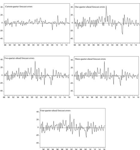
Column 1 of Table 2 reports the estimates of α along with the correct t-values in rows 1–5. As indicated in bold, the null hypothesis that α = 0 is rejected for both f = 0 and 1. Thus, with the ME estimates (1.435 and 2.029) positive, the current-quarter and one-quarter-ahead forecasts, on average, significantly under-predict growth in durables spending. However, the null hypothesis cannot be rejected for f = 2, 3, and 4, meaning that the two- three-, and four-quarter-ahead forecasts do not, on average, significantly over- or under-predict. For these forecasts, the ME estimates (ranging from 1.003 to 1.073) are small, compared to the mean absolute forecast error (MAE) estimates (ranging from 6.955 to 7.582), reported in column 2 (rows 3–5) of Table 2.

Table 2. Federal Reserve forecast accuracy results.

			MAE		Directional accuracy
$(A_{t+f}–P{F}_{t+f})=\alpha +u_{t+f}$	f	α = ME	PFt+f	PNt+f	πAll	πUp	πDown	p-value
Row no.		(1)	(2)	(3)	(4)	(5)	(6)	(7)
1	0	1.435 (2.91)	3.854	11.65	0.92^a	0.89	0.95	0.297
2	1	2.029 (2.18)	7.396	10.33	0.74^a	0.67	0.80	0.094
3	2	1.003 (1.19)	7.061	9.843	0.74^a	0.74	0.74	0.994
4	3	1.073 (1.23)	6.955	9.836	0.77^a	0.73	0.80	0.371
5	4	1.010 (1.17)	7.582	10.57	0.73^a	0.72	0.75	0.756

Note: The correct t-values are in parentheses. ME estimates in bold are significantly different from zero. Superscript a indicates that the null hypothesis of no association between (A_t+f – R_t−1) and (PF_t+f – R_t−1) is rejected at the lower than 1% level of significance.

Source: Author’s calculation.

4.3. Do the forecasts outperform the naïve forecasts?

The current-quarter and one- through four-quarter-ahead naïve forecasts (denoted PN_t+f) are set equal to real-time growth in durables spending belonging to quarter t−1 (which is available at the time when the Federal Reserve forecasts are prepared in quarter t). Columns 2 and 3 of Table 2 report, respectively, the MAEs of Federal Reserve forecasts (PF_t+f) and naïve forecasts (PN_t+f). As can be seen, the MAE of PF_t+f (ranging from 3.854 to 7.582) is well below the MAE of PN_t+f (ranging from 9.836 to 11.65) for every forecast horizon in rows 1–5. In testing the null hypothesis of equal forecast accuracy, we follow Baghestani (2021a) and regress the difference in the absolute errors of PF_t+f and PN_t+f on a constant. As such, the constant is the difference between the MAE of PF_t+f and the MAE of PN_t+f. The p-value of the correct t-value for testing the null hypothesis (that the constant equals zero) is below 0.001 for every forecast horizon, meaning that the null hypothesis is rejected in favour of the alternative that PF_t+f is significantly more accurate than PN_t+f.

4.4. Do the forecasts accurately predict directional change?

Henriksson and Merton (1981) propose a procedure for evaluating the directional accuracy of market-timing forecasts. This procedure has been widely used for evaluating the directional accuracy of economic and financial forecasts (Baghestani & Toledo, 2017; Sinclair et al., 2010). We define the actual change by (A_t+f – R_t−1) and the predicted change by (P_t+f – R_t−1), where R_t−1 is real-time growth in durables spending belonging to quarter t−1 (which is available at the time when the Federal Reserve forecasts are prepared in quarter t). The overall directional accuracy rate is π_All = (n₁ + n₂)/(n₁ + n₂ + n₃ + n₄), where n₁ (n₂) is the number of quarters in which the actual and predicted changes are both positive (negative), and n₃ (n₄) are the number of quarters in which the actual change is positive (negative) and the predicted change is negative (positive). As reported in column 4 of Table 2, the overall accuracy rate (π_All), ranging from 0.73 to 0.92, is quite high for every forecast in rows 1–5. We use Fisher’s exact test and the chi-square tests with and without Yate’s continuity correction in order to test the null hypothesis of no association between (A_t+f – R_t−1) and (P_t+f – R_t−1). As shown by superscript a, this null hypothesis is rejected, meaning that the Federal Reserve forecasts accurately predict directional change.

Columns 5 and 6 of Table 2, further, report, respectively, the proportion of correctly predicted upward moves (π_Up = n₁/(n₁ + n₃)) and the proportion of correctly predicted downward moves (π_Down = n₂/(n₂ + n₄)). Column 7 reports the p-values of the chi-square test for the null hypothesis of no asymmetric loss (Berenson et al., 1988). As can be seen in row 2, π_Up (0.67) is far below π_Down (0.80) with a p-value of 0.094 < 0.10, meaning that the null hypothesis of no asymmetric loss is rejected. Accordingly, the one-quarter-ahead forecast is of value to a user who assigns high (low) cost to incorrectly predicted downward (upward) moves. However, for every forecast in rows 1 and 3–5, π_Up (ranging from 0.72 to 0.89) is similar to π_Down (ranging from 0.74 to 0.95). With the test p-values above 0.10, the null hypothesis of no asymmetric loss cannot be rejected. This means that the current-quarter, two-, three- and four-quarter-ahead Federal Reserve forecasts imply symmetric loss and are of value to a user who assigns similar cost to both incorrectly predicted upward and downward moves.

4.5. Are the forecast errors orthogonal to changes in consumer buying attitudes?

In answering, we estimate the following orthogonality test equation, (2) $$\left(A_{t+f}–P{F}_{t+f}\right)\mathrm{}={\beta }_0+{\beta }_1{X}_{t-1}+u_{t+f}$$(2) where X represents consumer buying attitudes. The data on X are quarterly averages of monthly data for quarter t−1 and are available when the Federal Reserve forecasts are prepared in quarter t. Under the null hypothesis of orthogonality (β₁ = 0), either the Federal Reserve forecasts contain the information in X or such information is not relevant, and thus does not help reduce forecast errors. Table 3 reports the p-values of the correct t-value for testing the null hypothesis that β₁ = 0. More specifically, rows 1, 3, 5, and 7 report the test p-values for when X represents, respectively, durables-buying attitudes (DBA) of 35–54-year-old participants, participants with a college degree, male participants, and participants with the top 33% income. As can be seen, these p-values are above 0.10 (for all forecast horizons), meaning that the Federal Reserve forecast errors are orthogonal to the difference of opinion of consumers about whether now is a good time or a bad time to buy major household items (DBA). This means that the Federal Reserve forecasts contain past information in DBA, and, thus, such information does not help improve forecast accuracy.

Table 3. Orthogonality test results.

$(A_{t+f}–P{F}_{t+f})\mathrm{}={\beta }_0+{\beta }_1{X}_{t-1}+u_{t+f}$
Row no.	X	f = 0	f = 1	f = 2	f = 3	f = 4
		(1)	(2)	(3)	(4)	(5)
35–54-year-old participants
1	DBA	0.587	0.737	0.292	0.101	0.437
2	HBA	0.176	0.001	0.031	0.013	0.037
Participants with a college degree
3	DBA	0.876	0.926	0.349	0.144	0.540
4	HBA	0.460	0.054	0.083	0.091	0.073
Male participants
5	DBA	0.638	0.944	0.304	0.131	0.346
6	HBA	0.140	0.002	0.046	0.022	0.055
Participants with the top 33% income
7	DBA	0.738	0.998	0.533	0.166	0.529
8	HBA	0.243	0.013	0.045	0.092	0.081

Notes: Numbers are the p-values of the calculated correct t-values for testing the null hypothesis that β₁ = 0. Those below 0.10 are in bold.

Source: Author’s calculation.

Rows 2, 4, 6, and 8 of Table 3 report the test p-values for when X represents, respectively, home-buying attitudes (HBA) of 35–54-year-old participants, participants with a college degree, male participants, and participants with the top 33% income. As can be seen, these p-values are below 0.10 for f = 1, 2, 3 and 4 (but not for f = 0). This means that the one- through four-quarter-ahead Federal Reserve forecast errors fail to be orthogonal to the difference of opinion of consumers about whether now is a good time or a bad time to buy a house and, thus, past information in HBA can potentially help improve forecast accuracy.

4.6. Do consumer home-buying attitudes and expectations help improve predictive accuracy?

Following the orthogonality test results in Table 3, we construct the following simple knowledge model (KM), (3) $$g_{\mathrm{t}}={\gamma }_0+{\gamma }_{1}HB{A}_{\mathrm{t}-1}+{\gamma }_{2}CE{B}_{\mathrm{t}-1}+v_t$$(3) where g_t is real-time growth in durables spending, HBA is consumer home-buying attitudes, and CEB is consumer expectations about future business conditions.² The data on HBA and CEB are quarterly averages of monthly data for quarter t−1 and are available when the Federal Reserve forecasts are prepared in quarter t. It is important to note that, as balance data, both HBA and CEB are differences as a percentage. For instance, the former measures the difference of opinion of consumers about whether now is a good or a bad time to buy a house, and the latter measures the difference of opinion of consumers about whether business conditions will be better or worse a year from now.

Rows 1, 3, and 5 (row 7) of Table 4 report, respectively, the 1978Q2–1987Q4 (1980Q1–1987Q4) estimates of (3) for 35–54-year-old participants, participants with a college degree, and male participants (participants with the top 33% income). As can be seen, the estimates of γ₁ and γ₂ have the theoretically correct (positive) signs and are significantly different from zero. The same is true for the sample periods ending 2015Q3 in rows 2, 4, 6, and 8 of Table 4.

Table 4. Knowledge model (KM) estimates of growth in durables spending.

$g_t={\gamma }_0+{\gamma }_{1}HB{A}_{\mathrm{t}-1}+{\gamma }_{2}CE{B}_{\mathrm{t}-1}+v_t$
Row no.	Sample period	γ0	γ1	γ2	R^2
35–54-year-old participants
1	1978Q2–1987Q4	−41.26 (2.73)	0.072 (1.65)	0.362 (2.72)	0.219
2	1978Q2–2015Q3	−35.58 (4.84)	0.054 (2.01)	0.312 (4.76)	0.178
Participants with a college degree
3	1978Q2–1987Q4	−42.86 (2.96)	0.104 (1.85)	0.321 (2.86)	0.245
4	1978Q2–2015Q3	−30.50 (4.31)	0.067 (2.37)	0.233 (4.17)	0.153
Male participants
5	1978Q2–1987Q4	−47.96 (2.97)	0.101 (1.73)	0.370 (2.95)	0.239
6	1978Q2–2015Q3	−34.81 (4.54)	0.073 (2.54)	0.265 (4.34)	0.161
Participants with the top 33% income
7	1980Q1–1987Q4	−58.47 (3.21)	0.083 (1.69)	0.455 (3.12)	0.303
8	1980Q1–2015Q3	−37.17 (4.71)	0.073 (2.80)	0.277 (4.58)	0.175

Note: g_t is real-time growth in durables spending, HBA is consumer home-buying attitudes, and CEB is consumer expectations about future business conditions. Numbers in parentheses are the absolute t-values. Coefficient estimates in bold are significantly different from zero. The data on HBA and CEB are available starting 1980Q1 for participants with the top 33% income.

Source: Author’s calculation.

In generating the KM forecasts (denoted PK_t+f), we use the 1978Q2–1987Q4 parameter estimates (of γ₀, γ₁, and γ₂) in order to calculate the fitted values. The current-quarter and one- through four-quarter-ahead KM forecasts are then set equal to the fitted value for 1987Q4. As such, these KM forecasts match the Federal Reserve forecasts made in 1988Q1. Re-estimating the model for 1978Q2–1988Q1, the updated parameter estimates are used to generate the fitted values. The current-quarter and one- through four-quarter-ahead forecasts are then set equal to the fitted value for 1988Q1. These KM forecasts match the Federal Reserve forecasts made in 1988Q2. We repeat this procedure until the last set of KM forecasts for 2015Q4–2016Q4 is generated using the 1978Q2–2015Q3 parameter estimates. Again, these KM forecasts match the Federal Reserve forecasts made in 2015Q4.³ Like the Federal Reserve forecasts, the sample periods for the current-quarter, one-, two-, three-, and four-quarter-ahead KM forecasts are, respectively, 1988Q1–2015Q4, 1988Q2–2016Q1, 1988Q3–2016Q2, 1988Q4–2016Q3, and 1989Q1–2016Q4, with 112 observations for every forecast horizon.

To compare the predictive information of the Federal Reserve and KM forecasts, the following encompassing test equation is estimated, (4) $$A_{t+f}={\mathrm{}\mathrm{\delta }}_0+{\mathrm{\delta }}_{1}P{F}_{t+f}+{\mathrm{\delta }}_{2}P{K}_{t+f}+u_{t+f}$$(4) where PF_t+f and PK_t+f are, respectively, the Federal Reserve and KM forecasts of A_t+f. Following Fair and Shiller (1990), PF_t+f contains more predictive information than PK_t+f when the estimate of δ₁ is positive and significant and the estimate of δ₂ is either insignificant or negative. The two forecasts contain distinct predictive information when the estimates of δ₁ and δ₂ are both positive and significant, and they contain similar predictive information when the estimates of δ₁ and δ₂ are both insignificant.

Table 5 reports the parameter estimates of (4) along with the correct t-values. As can be seen for every group of participants in Table 5, the estimate of δ₁ is positive and significant for f = 0, 1, 2, and 3, and the estimate of δ₂ is positive and significant for f = 1 and 4. These results lead to three conclusions. First, the one-quarter-ahead Federal Reserve and KM forecasts contain distinct predictive information. Second, the four-quarter-ahead KM forecast embodies useful predictive information above and beyond that contained in the Federal Reserve forecast. Third, the current-quarter, two- and three-quarter-ahead Federal Reserve forecasts are more accurate than the KM forecasts in terms of the predictive information content.

Table 5. Encompassing test results.

$A_{t+f}=\mathrm{}{\delta }_0+{\delta }_{1}P{F}_{t+f}+{\delta }_{2}P{K}_{t+f}+u_{t+f}$
Row no.	f	δ0	δ1	δ2	R^2
35–54-year-old participants
1	0	0.950 (0.89)	0.952 (16.6)	0.104 (0.74)	0.713
2	1	−0.444 (0.23)	0.418 (2.62)	0.685 (3.04)	0.153
3	2	−0.075 (0.03)	0.629 (2.15)	0.423 (1.61)	0.079
4	3	−1.147 (0.50)	0.901 (3.54)	0.398 (1.59)	0.122
5	4	1.371 (0.57)	0.352 (1.47)	0.415 (1.65)	0.053
Participants with a college degree
6	0	1.029 (0.97)	0.956 (17.0)	0.082 (0.65)	0.712
7	1	−0.432 (0.21)	0.419 (2.66)	0.622 (2.72)	0.133
8	2	0.136 (0.05)	0.588 (2.03)	0.383 (1.49)	0.071
9	3	−0.781 (0.35)	0.861 (3.37)	0.341 (1.50)	0.112
10	4	1.125 (0.47)	0.266 (1.11)	0.471 (1.86)	0.056
Male participants
11	0	0.797 (0.78)	0.952 (17.6)	0.123 (0.96)	0.714
12	1	−0.230 (0.13)	0.451 (2.93)	0.614 (2.58)	0.140
13	2	0.141 (0.06)	0.615 (2.12)	0.388 (1.59)	0.075
14	3	−0.712 (0.32)	0.896 (3.56)	0.326 (1.45)	0.113
15	4	1.480 (0.62)	0.340 (1.45)	0.395 (1.66)	0.051
Participants with the top 33% income
16	0	0.851 (0.95)	0.951 (17.7)	0.125 (1.10)	0.714
17	1	0.357 (0.21)	0.435 (2.83)	0.570 (2.81)	0.142
18	2	0.916 (0.21)	0.552 (1.88)	0.340 (1.44)	0.071
19	3	0.092 (0.05)	0.840 (3.14)	0.266 (1.29)	0.108
20	4	2.195 (1.09)	0.211 (0.87)	0.411 (1.83)	0.056

Notes: Coefficient estimates in bold are significantly different from zero.

Source: Author’s calculation.

Table 6 reports the MAEs of the Federal Reserve and KM forecasts in columns 1 and 2. As can be seen for every group of participants, the MAEs of the Federal Reserve forecasts are lower than the MAEs of the KM forecasts for f = 0, 2, and 3, and the MAEs of the KM forecasts are lower than the MAEs of the Federal Reserve forecasts for f = 1 and 4. Given these results, we next examine whether combining the two forecasts can help improve forecast accuracy.

Table 6. Mean absolute errors (MAE) of alternative forecasts.

Row no.	f	PFt+f	PKt+f	PCt+f	p-value
		(1)	(2)	(3)	(4)
35–54-year-old participants
1	0	3.854	7.518	4.989	–
2	1	7.396	7.212	6.744	0.051
3	2	7.061	7.367	7.016	0.838
4	3	6.955	7.403	6.814	0.476
5	4	7.582	7.317	7.105	0.021
Participants with a college degree
6	0	3.854	7.731	5.023	–
7	1	7.396	7.314	6.812	0.086
8	2	7.061	7.462	7.052	0.965
9	3	6.955	7.472	6.886	0.709
10	4	7.582	7.355	7.143	0.022
Male participants
11	0	3.854	7.590	5.043	–
12	1	7.396	7.331	6.806	0.087
13	2	7.061	7.404	7.056	0.961
14	3	6.955	7.480	6.890	0.737
15	4	7.582	7.415	7.122	0.026
Participants with the top 33% income
16	0	3.854	7.688	5.074	–
17	1	7.396	7.285	6.815	0.090
18	2	7.061	7.343	7.060	0.999
19	3	6.955	7.490	6.924	0.871
20	4	7.582	7.400	7.194	0.035

Notes: PF_t+f and PK_t+f are, respectively, the Federal Reserve and KM forecasts. PC_t+f is the combined forecasts. The p-values in column 4 are for testing the null hypothesis that the MAE of PC_t+f equals the MAE of PF_t+f. P-values below .10 are in bold.

Source: Author’s calculation.

The combined forecasts (denoted PC_t+f) are obtained by assigning equal weights to both the Federal Reserve and KM forecasts. Assigning equal weights follows the recommendation of Graefe (2015) and Green and Armstrong (2015), among others. Column 3 reports the MAEs of the combined forecasts. As can be seen for every group of participants, the MAEs of the combined forecasts are lower than the MAEs of the Federal Reserve forecasts for f = 1, 2, 3, and 4. In testing the null hypothesis of equal forecast accuracy, we regress the difference in the absolute errors of PF_t+f and PC_t+f on a constant. As such, the constant is the difference between the MAE of PF_t+f and the MAE of PC_t+f. The p-value of the correct t-value for testing the null hypothesis (that the constant equals zero) is reported in column 4. As can be seen, the p-values for f = 1 and 4 (in bold) are below 0.10, meaning that the null hypothesis is rejected in favour of the alternative that PC_t+1 (PC_t+4) is significantly more accurate than PF_t+1 (PF_t+4). Put together, the results indicate that home-buying attitudes and expectation about future business conditions (of 35–54-year-old participants, participants with a college degree, male participants, and participants with the top 33% income) help significantly reduce the one- and four-quarter-ahead Federal Reserve forecast errors.

To augment these results, columns 1 and 2 of Table 7 report the ME and MAE estimates of the one- and four-quarter-ahead combined forecasts (PC_t+1 and PC_t+4). As can be seen for every group of participants, these forecasts do not significantly over- or under predict growth in durables spending. For instance, the ME estimates are not significantly different from zero, and they are small compared to the MAE estimates. Columns 3–6 report, respectively, π_All, π_Up, π_Down in addition to the p-value for testing the null hypothesis of no asymmetric loss. As can be seen for every group of participants, the one- and four-quarter-ahead combined forecasts predict directional change with high accuracy rates under symmetric loss.

Table 7. Accuracy results of the combined (PC_t+f) forecasts.

$(A_{t+f}–P{C}_{t+f})\mathrm{}=\alpha +u_{t+f}$ Row no.	f			Directional accuracy
		α = ME	MAE	πAll	πUp	πDown	p-value
		(1)	(2)	(3)	(4)	(5)	(6)
35–54-year-old participants
1	1	0.516 (0.61)	6.744	0.73^a	0.75	0.72	0.777
2	4	0.083 (0.11)	7.105	0.79^a	0.77	0.80	0.717
Participants with a college degree
3	1	0.212 (0.25)	6.812	0.74^a	0.78	0.70	0.339
4	4	−0.221 (0.28)	7.143	0.76^a	0.79	0.73	0.442
Male participants
5	1	0.414 (0.49)	6.806	0.72^a	0.73	0.72	0.961
6	4	−0.020 (0.03)	7.122	0.79^a	0.77	0.82	0.545
Participants with the top 33% income
7	1	0.655 (0.77)	6.815	0.74^a	0.76	0.72	0.602
8	4	0.222 (0.28)	7.194	0.78^a	0.75	0.80	0.562

Note: See Table 2 notes.

Source: Author’s calculation.

Comparing the results in Table 7 with those in Table 2 for the Federal Reserve forecasts leads to three conclusions. First, on average, the one-quarter-ahead Federal Reserve forecasts significantly under-predict, while the combined forecasts do not significantly over- or under-predict growth in durables spending. Second, the one-quarter-ahead Federal Reserve forecast implies asymmetric loss, while the combined forecast implies symmetric loss and is thus of value to a user who assigns similar cost (loss) to both incorrectly predicted upward and downward moves. Third, the four-quarter-ahead combined forecast produces larger overall accuracy rates (ranging from 0.76 to 0.79) than the Federal Reserve forecast (0.73) in Table 2.

5. Discussion

Relevant to this study, there are three important points to note. First, accurate forecasts of growth in durables spending are important as input in designing monetary policy. Second, the psychological consumption theory maintains that consumer buying attitudes and expectations about future personal finances and overall business conditions influence consumer willingness to buy, which, in turn, affect purchases of durable goods (Baghestani & Fatima, 2021). Third, research shows that consumer survey responses vary substantially across demographics, and disaggregation by age, education, gender, and income can help reveal useful information. The appeal for the use of such data in forecasting partly stems from the fact that they are available in real time and are not subject to revision (Easaw et al., 2005).

We show that, for 1988–2016, the Federal Reserve forecasts, while superior to the naïve benchmark, are directionally accurate. Directionally accurate forecasts of growth in durables spending, in particular, are crucial for implementing countercyclical policies (Easaw et al., 2005), since declines in such spending are considered a possible cause of recession (Blanchard, 1993). Further results indicate that, on average, the shorter-horizon Federal Reserve forecasts under-predict, but the longer-horizon forecasts do not significantly over- or under-predict growth in durables spending. In addition, these forecasts generally imply symmetric loss. The only exception is the one-quarter-ahead forecast, which implies asymmetric loss.

As for consumer survey data, the findings indicate that disaggregation helps reveal useful information embodied in the cross-sectional distribution of the data, and it is consistent with Souleles (2004) who shows that the positive effect of sentiment on consumption is partly due to heterogeneity at the household level. According to the orthogonality test results, for instance, the Federal Reserve forecasts do (do not) contain consumer durables-buying (home-buying) attitudes of 35–54-year-old participants, participants with a college degree, male participants, and participants with the top 33% income. Using real-time data on durables spending and the information in consumer home-buying attitudes and expectations, we constructed a knowledge model (KM) to generate comparable forecasts of growth in durables spending. Our results indicate that the one- and four-quarter-ahead KM forecasts can potentially help improve the accuracy of Federal Reserve forecasts. Further results indicate that the one- and four-quarter-ahead combined Federal Reserve and KM forecasts show significant reductions in forecast errors, meaning that there are accuracy gains from using disaggregated consumer survey data. Thus, the practical implication is that forecasters should pay special attention to consumer home-buying attitudes and expectations about future business conditions, and policymakers should make use of such survey measures in monitoring the economy in real time.

6. Conclusions

This study adds to the literature by first evaluating the Federal Reserve forecasts of growth in durables spending and then showing that there are accuracy gains from using disaggregated home-buying attitudes and expectations about future business conditions. Our analysis further shows that consumer durables-buying attitudes, which measure the difference of opinion of consumers about whether now is a good or a bad time to buy a house, do not help improve forecast accuracy. One question that remains unanswered is whether the Federal Reserve forecasts can be improved using consumer responses to the follow-up questions, which emphasize important factors. For instance, for the participants who respond that it is a good time to buy major household items, there are five options to select as reasons: ‘Prices are low (good buys available), prices won’t come down, interest rate is low (credit easy), borrow in advance (rising rates), and times are good (prosperity).’ For the participants who respond that it is a bad time to buy major household items, there are four options to select as reasons: ‘Prices are high, interest rates are high (credit tight), cannot afford to buy, and uncertain future.’⁴ As to whether consumer responses to these follow-up questions help improve the accuracy of the Federal Reserve forecasts awaits subsequent research.

Disclaimer

This paper represents the opinions of the author and does not mean to represent the position or opinions of the American University of Sharjah.

Acknowledgement

The author would like to thank three anonymous reviewers for their helpful comments and suggestions.

Disclosure statement

This is to acknowledge that NO financial interest or benefit has arisen from the direct applications of this research.

Additional information

Funding

The work in this paper was supported, in part, by the Open Access Program from the American University of Sharjah.

Notes

1 ICS is constructed using three current-looking questions and two forward-looking questions. Some empirical models of consumer behavior include the dynamic relationship between the current- and forward-looking components of ICS (Baghestani, 2016; Baghestani & Palmer, 2017).

2 Real-time data on durables spending (DS) come from the Federal Reserve Bank of Philadelphia website. The growth rate is g_t = 100×((DS_t ÷ DS_t-1)⁴ –1).

3 The data on HBA and CEB are available starting 1980 for participants with the top 33% income. As such, the sample periods for generating the KM forecasts for these participants start from 1980 (instead of 1978).

4 The data for the follow-up questions are all available on the MSC website.

References

- Al-Eyd, A., Barrell, R., & Davis, E. P. (2009). Consumer confidence indices and short‐term forecasting of consumption. The Manchester School, 77, 96–111. https://doi.org/10.1111/j.1467-9957.2008.02089.x
- Armstrong, J. S., & Green, K. C. (2018). Forecasting methods and principles: Evidence-based checklists. Journal of Global Scholars of Marketing Science, 28(2), 103–159. https://doi.org/10.1080/21639159.2018.1441735
- Baghestani, H. (2006). Federal Reserve vs. private forecasts of real net exports. Economics Letters, 91(3), 349–353. https://doi.org/10.1016/j.econlet.2005.12.009
- Baghestani, H. (2011). Federal Reserve and private forecasts of growth in investment. Journal of Economics and Business, 63(4), 290–305. https://doi.org/10.1016/j.jeconbus.2010.08.004
- Baghestani, H. (2013a). Evaluating Federal Reserve predictions of growth in consumer spending. Applied Economics, 45(13), 1637–1646. https://doi.org/10.1080/00036846.2011.633893
- Baghestani, H. (2013b). On the accuracy of Federal Reserve forecasts of the saving rate. Applied Economics Letters, 20(18), 1651–1655. https://doi.org/10.1080/13504851.2013.831164
- Baghestani, H. (2016). Do gasoline prices asymmetrically affect US consumers’ economic outlook? Energy Economics, 55, 247–252. https://doi.org/10.1016/j.eneco.2016.02.012
- Baghestani, H. (2017a). Do consumers’ home buying attitudes explain the behaviour of US home sales? Applied Economics Letters, 24(11), 779–783. https://doi.org/10.1080/13504851.2016.1229401
- Baghestani, H. (2017b). Do US consumer survey data help beat the random walk in forecasting mortgage rates? Cogent Economics & Finance, 5(1), 1343017. https://doi.org/10.1080/23322039.2017.1343017
- Baghestani, H. (2020). Is there a gender difference in accurately predicting the sign of growth in durables spending? Applied Economics Letters, 27(5), 383–386. https://doi.org/10.1080/13504851.2019.1616060
- Baghestani, H. (2021a). Forecasts of growth in US residential investment: Accuracy gains from consumer home-buying attitudes and expectations. Applied Economics, 53(32), 3744–3758. https://doi.org/10.1080/00036846.2021.1885613
- Baghestani, H. (2021b). Predicting growth in US durables spending using consumer durables-buying attitudes. Journal of Business Research, 131, 327–336. https://doi.org/10.1016/j.jbusres.2021.03.025
- Baghestani, H., & AbuAl-Foul, B. M. (2017). Comparing Federal Reserve, Blue Chip, and time series forecasts of US output growth. Journal of Economics and Business, 89, 47–56. https://doi.org/10.1016/j.jeconbus.2016.11.001
- Baghestani, H., & Fatima, S. (2021). Growth in US durables spending: Assessing the impact of consumer ability and willingness to buy. Journal of Business Cycle Research, 17(1), 55–69. https://doi.org/10.1007/s41549-021-00053-7
- Baghestani, H., Kaya, I., & Kherfi, S. (2013). Do changes in consumers' home buying attitudes predict directional change in home sales? Applied Economics Letters, 20(5), 411–415. https://doi.org/10.1080/13504851.2012.709597
- Baghestani, H., & Palmer, P. (2017). On the dynamics of US consumer sentiment and economic policy assessment. Applied Economics, 49(3), 227–237. https://doi.org/10.1080/00036846.2016.1194964
- Baghestani, H., & Poulson, B. (2012). Federal Reserve forecasts of nonfarm payroll employment across different political regimes. Journal of Economic Studies, 39(3), 280–289. https://doi.org/10.1108/01443581211245874
- Baghestani, H., & Toledo, H. (2017). Do analysts' forecasts of term spread differential help predict directional change in exchange rates? International Review of Economics & Finance, 47, 62–69. https://doi.org/10.1016/j.iref.2016.10.003
- Baghestani, H., & Viriyavipart, A. (2019). Do factors influencing consumer home-buying attitudes explain output growth? Journal of Economic Studies, 46(5), 1104–1115. https://doi.org/10.1108/JES-01-2018-0040
- Berenson, M. L., Levine, D. M., & Rindskopf, D. (1988). Applied statistics: A first course. Prentice-Hall, Inc.
- Binder, C. C. (2015). Whose expectations augment the Phillips curve? Economics Letters, 136, 35–38. https://doi.org/10.1016/j.econlet.2015.08.013
- Blanchard, O. (1993). Consumption and the recession of 1990-1991. The American Economic Review, 83(2), 270–274.
- Bruestle, S., & Crain, W. M. (2015). A mean-variance approach to forecasting with the consumer confidence index. Applied Economics, 47(23), 2430–2444. https://doi.org/10.1080/00036846.2015.1008763
- Capistrán, C. (2008). Bias in Federal Reserve inflation forecasts: Is the Federal Reserve irrational or just cautious? Journal of Monetary Economics, 55(8), 1415–1427. https://doi.org/10.1016/j.jmoneco.2008.09.011
- Carruth, A., & Henley, A. (1992). Consumer durables spending and housing market activity. Scottish Journal of Political Economy, 39(3), 261–271. https://doi.org/10.1111/j.1467-9485.1992.tb00620.x
- Croushore, D. (2005). Do consumer-confidence indexes help forecast consumer spending in real time? The North American Journal of Economics and Finance, 16(3), 435–450. https://doi.org/10.1016/j.najef.2005.05.002
- Easaw, J. Z., Garratt, D., & Heravi, S. M. (2005). Does consumer sentiment accurately forecast UK household consumption? Are there any comparisons to be made with the US? Journal of Macroeconomics, 27(3), 517–532. https://doi.org/10.1016/j.jmacro.2004.03.001
- Erceg, C., & Levin, A. (2006). Optimal monetary policy with durable consumption goods. Journal of Monetary Economics, 53(7), 1341–1359. https://doi.org/10.1016/j.jmoneco.2005.05.005
- Fair, R. C., & Shiller, R. J. (1990). Comparing information in forecasts from econometric models. The American Economic Review, 80(3), 375–389.
- Faust, J., & Wright, J. H. (2013). Forecasting inflation. In: Graham E. and Timmermann, A. (Eds.), Handbook of economic forecasting, 22–56. North-Holland.
- Garner, C. A. (1981). Economic determinants of consumer sentiment. Journal of Business Research, 9(2), 205–220. https://doi.org/10.1016/0148-2963(81)90004-7
- Gavin, W. T., & Mandal, R. J. (2003). Evaluating FOMC forecasts. International Journal of Forecasting, 19(4), 655–667. https://doi.org/10.1016/S0169-2070(02)00075-4
- Graefe, A. (2015). Improving forecasts using equally weighted predictors. Journal of Business Research, 68(8), 1792–1799. https://doi.org/10.1016/j.jbusres.2015.03.038
- Green, K. C., & Armstrong, J. S. (2015). Simple versus complex forecasting: The evidence. Journal of Business Research, 68(8), 1678–1685. https://doi.org/10.1016/j.jbusres.2015.03.026
- Gupta, R., Marco Lau, C. K., Plakandaras, V., & Wong, W. K. (2019). The role of housing sentiment in forecasting US home sales growth: Evidence from a Bayesian compressed vector autoregressive model. Economic Research-Ekonomska Istraživanja, 32(1), 2554–2567. https://doi.org/10.1080/1331677X.2019.1650657
- Henriksson, R. D., & Merton, R. C. (1981). On market timing and investment performance. II. Statistical procedures for evaluating forecasting skills. The Journal of Business, 54(4), 513–533. https://doi.org/10.1086/296144
- Jennings, E. J., & McGrath, P. (1994). The influence of consumer sentiment on the sales of durables. The Journal of Business Forecasting, 13(3), 17–21.
- Joutz, F., & Stekler, H. O. (2000). An evaluation of the predictions of the Federal Reserve. International Journal of Forecasting, 16(1), 17–38. https://doi.org/10.1016/S0169-2070(99)00046-1
- Katona, G. (1975). Psychological economics. Elsevier Scientific Publishing Co.
- Kwan, A. C., & Cotsomitis, J. A. (2006). The usefulness of consumer confidence in forecasting household spending in Canada: A national and regional analysis. Economic Inquiry, 44(1), 185–197. https://doi.org/10.1093/ei/cbi064
- Lahiri, K., Monokroussos, G., & Zhao, Y. (2016). Forecasting consumption: The role of consumer confidence in real time with many predictors. Journal of Applied Econometrics, 31(7), 1254–1275. https://doi.org/10.1002/jae.2494
- Ludvigson, S. C. (2004). Consumer confidence and consumer spending. Journal of Economic Perspectives, 18(2), 29–50. https://doi.org/10.1257/0895330041371222
- Lunsford, K. G. (2015). Forecasting residential investment in the United States. International Journal of Forecasting, 31(2), 276–285. https://doi.org/10.1016/j.ijforecast.2014.07.004
- Mankiw, N. G., Reis, R., & Wolfers, J. (2003). Disagreement about inflation expectations. NBER Macroeconomics Annual, 18, 209–248. https://doi.org/10.1086/ma.18.3585256
- Romer, C. D., & Romer, D. H. (2000). Federal Reserve information and the behavior of interest rates. American Economic Review, 90(3), 429–457. https://doi.org/10.1257/aer.90.3.429
- Sinclair, T. M., Stekler, H. O., & Kitzinger, L. (2010). Directional forecasts of GDP and inflation: A joint evaluation with an application to Federal Reserve predictions. Applied Economics, 42(18), 2289–2297. https://doi.org/10.1080/00036840701857978
- Souleles, N. S. (2004). Expectations, heterogeneous forecast errors, and consumption: Micro evidence from the Michigan consumer sentiment surveys. Journal of Money, Credit, and Banking, 36(1), 39–72. https://doi.org/10.1353/mcb.2004.0007