Nexus between energy pricing and carbon emission. A policy mix response of developing economies

Abstract

The study utilised a data set of South Asian countries of energy pricing (E.P.), carbon emission, and policy mix between 1990 and 2020. A comprehensive set of models from econometric such as fixed effect (F.E.), and panel quantile regression (P.Q.R.) is used to determine the relationship between underline indicators. Furthermore, the T.O.P.S.I.S. method from operational research was applied to determine the efficiency level of these factors in the South Asian region. E.P. and carbon emission are contributing positively to the process of household consumption (H.C.). In the policy mix scenario, H.C. is positively associated with inflation while negatively with the tax rate. Furthermore, the outcomes of the T.O.P.S.I.S. indicate that Bhutan is performing efficiently in the said parameters followed by Pakistan, while India’s performance is not impressive in this regard. This study can be helpful to policymakers for effective energy demand planning, conservation, and frame policies that would ensure sustainable H.C. and serve as motivation to search for alternative energy sources to meet the growing energy demand.

Keywords:

• energy prices
• fixed effect (F.E.) model
• carbon emission
• policy mix
• developing economies

JEL CLASSIFICATIONS:

• C31
• C33
• C44
• H2
• H3
• Q41
• Q51

1. Introduction

Energy is likely to be one of the biggest concerns of this century, especially in the age of globalisation. It is a source of productive activities such as agriculture, trade, manufacturing, and industry. Along with the energy cycle, all economic sectors are interconnected, and a change in the energy price range significantly impacts the economy (Abbas et al., 2020). Especially in developing countries, commodity prices are considered more complex than regular prices. Furthermore, energy contributes to reducing poverty and hunger through economic growth and prosperity (Diawuo et al., 2020). Therefore, energy is needed to regard as an essential indicator for maintaining the economy. However, the traditional growth theory labelled labour and capital as the critical production drivers, ignoring the energy’s significance in the development process (Warr & Ayres, 2012). Thus, recent research emphasises the importance of energy in countries’ production and consumption functions (Fang & Chang, 2016). Energy demand is expected to increase in developing economies, especially across South Asia, due to the growing population and industrialisation (Notarnicola et al., 2017). However, rational prices are considered a prerequisite for promoting energy efficiency and achieving sustainable development goals (S.D.G.s-2030).

The South Asia region consists of developing economies with a lot of economic and social constraints. This region is a homeland of 1.94 billion people; however, more than 40% live below the poverty line (Halff et al., 2019). Regional countries are the net oil importers, and barriers to oil supply have crippled this region by imposing import bills. Higher oil prices reduce real wealth and consumer spending. The overall welfare of the oil-importing countries is expected to reduce oil prices by 20% (Yeh et al., 2021). Ghorbani et al. (2018) stated that rising prices of energy sources such as fuel, gas, and electricity harm the well-being of consumers. Therefore, both income and cost are the significant factors of consumer welfare. Other factors like environmental degradation and social vulnerabilities are the most emerging issues (Halbac-Cotoara-Zamfir et al., 2020). The monetary and fiscal policies (policy mix after that) are considered the real challenges for the region due to high fluctuations in the exchange rate, high demand for dollars for oil bills payments, current account deficit, and negative balance of payment (Omojolaibi & Egwaikhide, 2014).

Better utilisation of energy resources saves time while also contributing to a better quality of life and a healthier environment for everyone involved. It improves the efficient use of modern medical equipment and provides better educational facilities such as social services. There are substantial economic, political, and societal obstacles to energy price reform plans that complement the country without considering the repercussions (Natalini et al., 2020). Consequences of uniformly applied subsidies and price reform include that no two households receive the same subsidies or experience the same price and income changes. Reducing energy import costs is a top priority for policymakers in countries where energy costs are changing rapidly (Ali et al., 2018). Therefore, increasing energy prices eliminates effective solutions to social and economic issues associated with secondary aspects of energy. However, removing domestic subsidies does not significantly impact energy use and, therefore, the environment, especially if households with high energy consumption have less elastic demand for domestic energy. Additionally, the subsidy policy could also be backward because the share of energy in low-income households is above that of high-income households.

The primary purpose of this study is to find fresh evidence of energy pricing (E.P.), carbon emission, and policy mix tools of the South Asian region. For this purpose, we utilised intensive methods like fixed effect (F.E.), panel quantile regression (P.Q.R.) of econometrics, and T.O.P.S.I.S. from operational research. The study is essential for policymakers and individuals to make their decision in energy consumption. It also provides a way for the government that make policies to control high energy prices.

1.1. Literature review

The role of E.P. in determining household consumption (H.C.) level has become crucial in the current time due to the high demand for importable energy sources. Rasaq Adejumobi and Olatunde Julius (2017) found that the recent rise in oil prices has generally severely affected the worldwide economy and oil-importing South Asian economies. Petroleum prices are firmly linked to the consequences of inflation and are steadily increasing over the past three decades, resulting in growing economic instability (Sun et al., 2020). Such growth in energy demand will burden shipping consumers of all kinds of fuel prices (Al Mamun et al., 2014). The high oil price of $100/barrel will affect the domestic economy, and it is often a drag for oil-importing or low-income countries. Rekha Manjunath et al. (2020) considered demand, supply, and exchange rate as critical factors determining the changes in oil prices within the international and domestic markets. The petroleum prices lead to disruption of developing economies by vulnerable of the local exchange rate against the U.S. dollar. Therefore, the biggest reason for the high energy prices is the dollar’s appreciation against local currencies (Murad et al., 2019).

On the other hand, Cantore and Freund (2021) considered the fiscal parameters in H.C. determine. However, macroeconomic policy or policy mix is considered an essential tool for consumption stability. Chan (2020) found that all the policies as mentioned above could stabilise carbon emissions, their underlying mechanisms. Fiscal, monetary, and carbon tax policies uniquely and respectively reduce abatement effort, income tax revenue, and general price level (Tang et al., 2014). The economic expansions driven by total factor productivity shocks, policy mix can be the way to maintain the emission levels and simultaneously improve household welfare in terms of consumption and labour (Iqbal et al., 2020). Therefore, mechanical, political, and monetary changes to build up administration proficiency and remote guide put resources into advancement plans to enhance the economic process. This study considered the relationship among policy mix, E.P., environmental sustainability, and consumption pattern of the South Asian region.

2. Theoretical background and evaluation modelling

This study analyses the data set of six South Asian economies, namely, India, Pakistan, Bangladesh, Bhutan, and Sri Lanka, from 1990 to 2020. The variable description and their respective sources are given in Table 1 below.

Table 1. Variable description and data sources.

Variables	Description	Measurement	Data source
Household consumption	(HC)	Household final consumption as a % of GDP.	World Development Indicator (WDI) 2020 & OECD
Carbon dioxide emissions	(CO2)	Value-added	International Energy Agency (IEA), 2020
Energy (fuel) prices	(EP)	Fuel price (US$ per liter)	German Agency for International Cooperation (GIZ).
Per capita income	(PCI)	Adjusted net national income per capita (annual % growth)	World Development Indicator (WDI) 2020
Tax rate	(TAX)	Taxes on income, profits, and capital gains (% of total taxes)	IMF, International Financial Statistics
Inflation rate	(INF)	Inflation, consumer prices (annual %)	IMF, International Financial Statistics

For this table, last column provide the comprehensive detail of all sources where the dataset have been generated.

We divided our modelling section into two parts: econometric analysis and operational research. We utilised the F.E. model and panel quantile regression (P.Q.R.) from the econometric side.

For the data diagnostic process, we used second-generation unit root to view the stationarity trend in our data set. The second generation of panel unit root tests can overcome the shortcoming of cross-sectional dependence in the first-generation tests. With regards to this, except for Bai and Ng (2005) and Harris et al. (2005), all the tests assume that there is a unit root in the data. The second-generation tests are based on the heterogeneity assumption. Accordingly, there is no common autoregressive (A.R.) structure in the series and the panels are heterogeneous.

We applied Im et al.’s (2003) unit root test: (1) $$\mathrm{IPS}=\frac{\sqrt{\mathrm{N}}\left\{\mathrm{t}-\text{bar NT}-\mathrm{E}\left(\mathrm{\tau }\mathrm{T}\right)\right\}}{\sqrt{\mathrm{V}\mathrm{ar}\left(\mathrm{\tau }\mathrm{T}\right)}}$$(1)

In Equation 1(1) $$\mathrm{IPS}=\frac{\sqrt{\mathrm{N}}\left\{\mathrm{t}-\text{bar NT}-\mathrm{E}\left(\mathrm{\tau }\mathrm{T}\right)\right\}}{\sqrt{\mathrm{V}\mathrm{ar}\left(\mathrm{\tau }\mathrm{T}\right)}}$$(1) , $t-\mathit{bar}\mathrm{}NT=N^{-1}{\sum }_{i=1}^N\tau iT$ is the ratio of t of ADF(p) regression of the i^th croscross-sectiont. $E(\tau T)$ and $\mathit{Var}(\tau T)$ are the mean and variance of $\tau iT.$ They still don’t compensate for cross-sectional dependence in the error term, which is a major shortcoming of these tests. As a result, we use the cross-sectionally-augmented I.P.S. (C.I.P.S.) regression derived from the cross-sectionally augmented A.D.F. (C.A.D.F.) regression to verify the series’ stationarity. The C.A.D.F. regression can be expressed as: (2) $$\Delta {\mathrm{x}}_{\mathrm{it}}={\mathrm{z}}_{\mathrm{it}}^{\mathrm{\prime }}\mathrm{y}+{\mathrm{a}}_{\mathrm{i}{\mathrm{x}}_{\mathrm{it}-1}}+\sum _{\mathrm{j}=0}^{\mathrm{pi}}{\mathrm{\varnothing }}_{\mathrm{ij}}{\Delta \mathrm{x}}_{\mathrm{it}-\mathrm{j}}+{\mathrm{n}}_{\mathrm{i}}{\overline{\mathrm{X}}}_{\mathrm{it}-1}+\mathrm{}\sum _{\mathrm{j}=0}^{\mathrm{pi}}{\mathrm{\varnothing }}_{\mathrm{ij}}{\overline{\Delta \mathrm{X}}}_{\mathrm{it}-1}+{\mathrm{\epsilon }}_{\mathrm{it}}$$(2)

In Equation 2(2) $$\Delta {\mathrm{x}}_{\mathrm{it}}={\mathrm{z}}_{\mathrm{it}}^{\mathrm{\prime }}\mathrm{y}+{\mathrm{a}}_{\mathrm{i}{\mathrm{x}}_{\mathrm{it}-1}}+\sum _{\mathrm{j}=0}^{\mathrm{pi}}{\mathrm{\varnothing }}_{\mathrm{ij}}{\Delta \mathrm{x}}_{\mathrm{it}-\mathrm{j}}+{\mathrm{n}}_{\mathrm{i}}{\overline{\mathrm{X}}}_{\mathrm{it}-1}+\mathrm{}\sum _{\mathrm{j}=0}^{\mathrm{pi}}{\mathrm{\varnothing }}_{\mathrm{ij}}{\overline{\Delta \mathrm{X}}}_{\mathrm{it}-1}+{\mathrm{\epsilon }}_{\mathrm{it}}$$(2) , $x_{it}$ it is by the country mean across the time of interest. Individual country C.A.D.F. statistics comprise the cross-sectionally enhanced I.P.S., and Pesaran provides the crucial values for each one.

The Hausman Evaluation determines the suitability of the model whether the best model is an F.E. or a Random Effect (R.E.). If H₀ is true, then choose R.E. (p > 0.05) and if H₁ is true, then choose F.E. (p 0.05).

The Lagrangian Multiplier Test is a statistical procedure to evaluate whether the F.E. or R.E. is the optimal panel data regression approach. The Lagrange Multiplier test has a function to determine the best estimate, whether using an R.E. or not.

The F.E. Model indicates the unit’s only specific effect associated with the explanatory variables in the panel regression analysis. The F.E. model explains that quantities that are non-random and sample groups of the mean are considered a sample of the population in the model. In this model, data is generated into a group that is considered as various observed indicators. In panel data, the F.E. model identifies the subject-specific means and equation is given below: (3) $$Y_{it}={\alpha }_{\mathit{yxt}}{X}_{it}+{\alpha }_{\mathit{yzt}}{Z}_i+{\delta }_{\varpi }{\eta }_t+{\epsilon }_{it}$$(3)

The econometric model will be applied based on the unit root test. Our model is given below: (4) $$HC={\beta }_0+{\beta }_{1}PCI+{\beta }_{2}EP+{\beta }_{3}CO2+{\beta }_{4}INF+{\beta }_{5}TAX+{\epsilon }_{it}$$(4)

In Equation 4(4) $$HC={\beta }_0+{\beta }_{1}PCI+{\beta }_{2}EP+{\beta }_{3}CO2+{\beta }_{4}INF+{\beta }_{5}TAX+{\epsilon }_{it}$$(4) , HC is household consumption, PCI, per capita national income, EP, energy prices, INF, inflation, tax rate, CO₂, carbon omission, and ε is an error term.

Furthermore, the Quintile analysis research conducted in the past has often estimated a conditional mean model with F.E. The generalised expression of this is presented in Equation 5(5) $$E\mathrm{}\left(y_{it}\mathrm{}\mathrm{ǀ}{x}_{it,\mathrm{}}{\alpha }_{it}\right)\mathrm{}=\mathrm{}{x}_{it}^T\mathrm{}\beta +\mathrm{}{\alpha }_i$$(5) : (5) $$E\mathrm{}\left(y_{it}\mathrm{}\mathrm{ǀ}{x}_{it,\mathrm{}}{\alpha }_{it}\right)\mathrm{}=\mathrm{}{x}_{it}^T\mathrm{}\beta +\mathrm{}{\alpha }_i$$(5)

In this case, $y_{it}$ represents the logarithm of i^th country TA number at year $t,$ $x_{it}\mathrm{}=\mathrm{}{\left(x_{it,1}^T\mathrm{},\mathrm{}..\mathrm{},\mathrm{}{x}_{it,p}^T\right)}^T\mathrm{}$is $ap\mathrm{}\times \mathrm{}1$ vector of explanatory variables is represented by T and the (unobserved) county impact is denoted by ${\alpha }_i,$ which adjusts for time-invariant components of unobserved heterogeneity. The ordinary least squares (O.L.S.) do not assure that the error terms have a normal distribution, leading to inaccurate results. A quintile regression strategy is better in this case since the residual series are non-normal, and the results are robust to outlier and heavy-tail distributions (Ben Rejeb, 2017). Accordingly, this research estimates a conditional quantile regression model with F.E.s while considering the traditional linear function. (6) $${\mathrm{HC}}_{\mathrm{yit}}\mathrm{}\left(\mathrm{\daleth }\mathrm{ǀ}{\mathrm{x}}_{\mathrm{it},\mathrm{}}{\mathrm{\alpha }}_{\mathrm{it}}\right)={\mathrm{\beta }}_{1\mathrm{\daleth }}\mathrm{P}\mathrm{C}{\mathrm{I}}_{\mathrm{it}}+{\mathrm{\beta }}_{2\mathrm{\daleth }}\mathrm{E}{\mathrm{P}}_{\mathrm{it}}+{\mathrm{\beta }}_{3\mathrm{\daleth }}\mathrm{}{\mathrm{CO}2}_{\mathrm{it}}+{\mathrm{\beta }}_{4\mathrm{\daleth }}{\mathrm{INF}}_{\mathrm{it}}\mathrm{}{+\mathrm{\beta }}_{5\mathrm{\daleth }}{\mathrm{TAX}}_{\mathrm{it}}+{\mathrm{\alpha }}_{\mathrm{i}}$$(6) (7) $$\mathrm{PC}{\mathrm{I}}_{\mathrm{T}}^{\mathrm{*}}\mathrm{}=\mathrm{}-\mathrm{}\frac{{\mathrm{\theta }}_{1\mathrm{\daleth }}}{{2\mathrm{\theta }}_{1\mathrm{\daleth }}}$$(7)

For example, the coefficients of linear and quadratic corruption at quantile are represented by the symbol’s theta ${\theta }_{1\mathrm{\daleth }}$ and ${\theta }_{2\mathrm{\daleth }}\mathrm{}$in Equation 7(7) $$\mathrm{PC}{\mathrm{I}}_{\mathrm{T}}^{\mathrm{*}}\mathrm{}=\mathrm{}-\mathrm{}\frac{{\mathrm{\theta }}_{1\mathrm{\daleth }}}{{2\mathrm{\theta }}_{1\mathrm{\daleth }}}$$(7) . According to Koenker and Bassett (1978), quantile regression was initially introduced in their seminal article as an expansion to a collection of models for distinct conditional quantile functions of the traditional estimation of the conditional mean. Assume that you want to minimise the ${\mathrm{\daleth }}^{th}$ regression quintile estimate $\widehat{\beta }(\mathrm{\daleth }).$ (8) $$\widehat{\beta }\left(\mathrm{\daleth }\right)=\underset{\mathit{\beta ϵ}{\mathfrak{R}}^k}{\arg }\mathrm{}\min \left[\sum _{i\mathrm{}ϵ\left\{i:y_{i\ge x_i}\mathrm{}\beta \right\}}\mathrm{\daleth }\mathrm{ǀ}{y}_{i\mathrm{}}-x_i\mathrm{}\beta \mathrm{ǀ}+\mathrm{}\sum _{i\mathrm{}ϵ\left\{i:y_{i\ge x_i}\mathrm{}\beta \right\}}\mathrm{}\left(1-\mathrm{\daleth }\mathrm{}\right)\mathrm{ǀ}{y}_i-x_i\mathrm{}\beta \mathrm{ǀ}\mathrm{}\right]$$(8)

Here in Equation 8(8) $$\widehat{\beta }\left(\mathrm{\daleth }\right)=\underset{\mathit{\beta ϵ}{\mathfrak{R}}^k}{\arg }\mathrm{}\min \left[\sum _{i\mathrm{}ϵ\left\{i:y_{i\ge x_i}\mathrm{}\beta \right\}}\mathrm{\daleth }\mathrm{ǀ}{y}_{i\mathrm{}}-x_i\mathrm{}\beta \mathrm{ǀ}+\mathrm{}\sum _{i\mathrm{}ϵ\left\{i:y_{i\ge x_i}\mathrm{}\beta \right\}}\mathrm{}\left(1-\mathrm{\daleth }\mathrm{}\right)\mathrm{ǀ}{y}_i-x_i\mathrm{}\beta \mathrm{ǀ}\mathrm{}\right]$$(8) , $\mathrm{\daleth }$ is a parameter $(0\mathrm{}<\mathrm{\daleth }<\mathrm{}1)$ which represents quintile size, the regression framework is designed using penalised P.Q.R. with F.E., and the penalised estimator is solved as follows: (9) $$\left(\widehat{\beta }\right({\mathrm{\daleth }}_k,\mathrm{}\mathrm{\lambda }),\mathrm{}\{{\alpha }_i\mathrm{},\left(\text{λ}\right)\}{\mathrm{}}_{i=1}^n\arg \mathrm{}\underset{\mathrm{}}{\min }\sum _{k=1\mathrm{}}^k\sum _{t=1\mathrm{}}^t\sum _{i=1\mathrm{}}^n{\omega }_k\mathrm{}{\rho }_{\mathrm{\daleth }k}\mathrm{}\left(y_{it}-x_{it}^T\mathrm{}\beta \mathrm{}{(\mathrm{\daleth }}_k\right)-{\alpha }_i)+\text{λ}\sum _{i=1\mathrm{}}^n\mathrm{ǀ}{\alpha }_i\mathrm{ǀ}\mathrm{}$$(9)

In Equation 9(9) $$\left(\widehat{\beta }\right({\mathrm{\daleth }}_k,\mathrm{}\mathrm{\lambda }),\mathrm{}\{{\alpha }_i\mathrm{},\left(\text{λ}\right)\}{\mathrm{}}_{i=1}^n\arg \mathrm{}\underset{\mathrm{}}{\min }\sum _{k=1\mathrm{}}^k\sum _{t=1\mathrm{}}^t\sum _{i=1\mathrm{}}^n{\omega }_k\mathrm{}{\rho }_{\mathrm{\daleth }k}\mathrm{}\left(y_{it}-x_{it}^T\mathrm{}\beta \mathrm{}{(\mathrm{\daleth }}_k\right)-{\alpha }_i)+\text{λ}\sum _{i=1\mathrm{}}^n\mathrm{ǀ}{\alpha }_i\mathrm{ǀ}\mathrm{}$$(9) , ${\rho }_{\mathrm{\daleth }k}\left(u\right)=u\left({\mathrm{\daleth }}_k-I\left(u\le 0\right)\right)$ is the conventional quantile scale parameter, ${\omega }_k$ is the left (kth) quantile loss function (Koenker, 2004). This weight regulates the kth quantile’s assessment approach to the F.E. statistical model. The segmentation of the predictor variables into subsets depends on its unbiased probability. The subsequent execution of an O.L.S. regression on these subsets is not a viable alternative to the quintile regression because significant systematic sampling concerns should be underlined (Koenker, 2017).

It is our intention in this article to use employ equally weighted quintiles ${\omega }_k=1/K$ (Alexander et al., 2011), where the tuning parameter is $\lambda .$ The punishment term $\lambda {\sum }_{i=1}^n\left|ai\right|\mathrm{}$ is used. A tuning parameter called $\lambda$ determines how much shrinkage is applied to each effect. We applied an F.E. model if the $\lambda =\mathrm{}0$ while can utilise disciplined method along with an F.E. model when $\lambda >0$ or $\lambda \to \mathrm{\infty }$ to acquire the P.Q.R. method. A simplified variance-minimising strategy of $\lambda$ is used in our empirical analysis. (10) $$\widehat{\lambda }=\mathit{arg}\underset{\lambda }{\inf }\left\{tr{\mathrm{\Sigma }}^{\mathrm{*}}\left({\beta }^{\mathrm{*}}\left(\mathrm{\daleth },\lambda \right),{\alpha }^{\mathrm{*}}\left(\lambda \right)\right)\right\}$$(10)

In Equation 10(10) $$\widehat{\lambda }=\mathit{arg}\underset{\lambda }{\inf }\left\{tr{\mathrm{\Sigma }}^{\mathrm{*}}\left({\beta }^{\mathrm{*}}\left(\mathrm{\daleth },\lambda \right),{\alpha }^{\mathrm{*}}\left(\lambda \right)\right)\right\}$$(10) , $tr{\mathrm{\Sigma }}^{\mathrm{*}}\left({\beta }^{\mathrm{*}}\left(\mathrm{\daleth },\lambda \right),{\alpha }^{\mathrm{*}}\left(\lambda \right)\right)$ is the trace of the covariance matrix achieved by the bootstrap technique.

Furthermore, the T.O.P.S.I.S. method can be utilised in this study. Its generalised form is presented in Equation 11(11) $${\mathrm{}S}_i^{+}=\sqrt{\sum _j^{11}{\left(d_{ij}-D_{\mathit{jbes}}^{+}\right)}^2}{\text{and}S}_i^{\mathrm{*}}=\sqrt{\sum _j^{11}{\left(d_{ij}-D_j^{\mathrm{*}}\right)}^2}$$(11) : (11) $${\mathrm{}S}_i^{+}=\sqrt{\sum _j^{11}{\left(d_{ij}-D_{\mathit{jbes}}^{+}\right)}^2}{\text{and}S}_i^{\mathrm{*}}=\sqrt{\sum _j^{11}{\left(d_{ij}-D_j^{\mathrm{*}}\right)}^2}$$(11)

$D^{\mathrm{*}}\mathrm{}=\mathrm{}\{d_1^{\mathrm{*}}\mathrm{},\mathrm{}{d}_2^{\mathrm{*}},\mathrm{}\cdots ,\mathrm{}{d}_{11}^{\mathrm{*}}\}\mathrm{}(\mathit{where}\mathrm{}{d}_j^{\mathrm{*}}\mathrm{}=\mathrm{}2d_{\mathit{jworst}}^{-}\mathrm{}-\mathrm{}{d}_{\mathit{jbes}}^{+})$ take over from the absolute harmful ideal solutions $D^{-}$ to avoid Euclidean distance invalidation. The relative closeness is defined as: $E_{\mathrm{}i}^{\mathrm{*}}=\frac{S_i^{+}}{S_i^{+}+S_i^{\mathrm{*}}}\mathrm{\hspace{0.5em}where}\mathrm{}0\mathrm{}\le \mathrm{}{E}_{\mathrm{}i}^{\mathrm{*}}\mathrm{}\le \mathrm{}0.1.$ The countries with $E_{\mathrm{}i}^{\mathrm{*}},$ in order of least to a most significant increase, are ranked.

3. Results

The estimation process for the said purpose is divided into three main parts. First, we did a diagnostic test of the data set. After that, we carried out a variable estimation process with the help of the econometric and operational research field. Finally, we did the model stability test for the estimation technique. Thus, Table 2 shows the data normalisation test based on Shapiro–Wilk.

Table 2. Shapiro–Wilk W test for normal data.

Variable	Obs	W	V	z	Prob > z
HC	186	0.94	8.22	4.83	0
EP	186	0.89	15.33	6.25	0
PCI	186	0.92	9.84	5.24	0
CO2	186	0.51	67.76	9.66	0
INF	186	0.89	15.01	6.20	0
TAX	186	0.89	14.05	6.05	0

Authors calculations based on STATA.

Table 2 represents the distribution of the sample. This test is used to the normality of distribution. The p-value is less than 5% (p<.05), indicating well-ordered and standardised sample quantiles fit the standard normal quantiles.

In the process of data diagnostic, the multicollinearity test is calculated by the Variance Inflation Factor (V.I.F.) given in Table 3. In this analysis, the ratio is calculated for each explanatory variable. A high V.I.F. value indicates the sign of multicollinearity in the model, usually greater than 5. According to the test outcomes, the V.I.F. for independent variables is less than 5. So, there is no issue of multicollinearity in the model.

Table 3. V.I.F. and Breusch–Pagan/Cook–Weisberg test for heteroskedasticity.

Variance inflation factor (VIF)
Variable	VIF	1/VIF
TAX	1.17	0.85
EP	1.16	0.85
PCI	1.13	0.88
CO2	1.12	0.89
INF	1.09	0.91
Mean VIF	1.14
Breusch–Pagan/Cook–Weisberg test for heteroskedasticity
Number of instruments = 165			Wald chi2(6) = 131.01
Prob > chi2 = 0.0000
Ho:	Constant variance
Variables:	fitted values of hc
chi2(1)	2.23
Prob > chi2	0.13

Authors calculations based on STATA.

Furthermore, the heteroskedasticity test is calculated by the Bruesch Pagan L.M. test in the lower part of Table 3. The null hypothesis is the constant variance that cannot be rejected because the p-value is more than 5%. So, variance is constant, and there is no heteroskedasticity in the model.

Accurate estimation of the data set requires constant mean and variance independent of time; moreover, this situation leads to the stationary of the data set. To determine such conditions, we applied the C.I.P.S., 2003 methods of a unit root.

Table 4 consists of the results of the C.I.P.S. test of the unit root test of each variable separately. All variables are stationary at the first difference, the order of integration is I(0), which indicates that there is no issue of a unit root. Therefore, we can utilise the F.E. method of estimation because variables are stationary at a level.

Table 4. Results of unit root tests.

Test based on CIPS
Variable	LEVEL		First difference		Order of integration
	Intercept	Trend and intercept	Intercept	Trend and intercept
HC	−3.39*	−3.15**	−6.82*	−4.97***	I(0)
EP	−0.75	−3.03***	−5.70*	−5.39***	I(0)
PCI	−2.19**	−1.46	−5.69*	−2.81***	I(0)
CO2	−2.09	−2.37	−4.23*	−3.40***	I(0)
INF	−3.26**	−3.55***	−3.49*	−5.19***	I(0)
TAX	−2.30*	−3.52***	−6.25*	5.59***	I(0)

H₀: indicates the stationary data set that is the null hypothesis (absence of unit root).

Critical values are 10%, 5%, and 2%, and values of LM less than critical values indicate the acceptance of H_o (null hypothesis). This is again the case data set has no unit root.

***, **, * Significant at 1%, 5%, and 10% level of significance.

Authors calculations based on STATA.

After carrying out the data diagnostic process, we utilised econometric and operational research techniques to determine the role of E.P., carbon emission, and policy mix tools (taxation, inflation) in H.C. in South Asia.

Table 5 presents the results of the F.E. According to the outcomes based on F.E., per capita income (P.C.I.) has a positive and significant impact on H.C. The p-value of P.C.I. is zero, which indicates that it is significant at 1%. The coefficient of the PCI indicates that a unit increase in P.C.I. can lead to a 0.4468-unit increase in H.C.

Table 5. Long-run results of regression.

Results of fixed effect model
Dependent variable: HC
	EP	PCI	CO2	INF	TAX	Cons
Coef.	0.3982***	0.4468***	0.5300***	0.5479***	−0.1378***	75.0163***
Std. Err.	0.1050	0.1010	0.1100	0.0903	0.0592	1.9616
t	3.9300	4.4200	0.0100	6.0800	−2.3200	38.2400
P>|t|	0.0040	0.0000	0.5780	0.0000	0.0210	0.0000
[95% Confidence Interval]	1.5721	0.64619	−4.3300	−0.3708	−0.2547	71.1449
	4.3686	0.24752	2.4200	0.7250	−0.0208	78.8878

Authors calculations based on STATA.

***, ** represent the significance level at 1% and 5%, respectively.

The F.E. model's fiscal policy tool (T.A.X.) coefficient has a significant impact with a negative sign. It indicates that a unit increase in tax level may reduce H.C. up to 13% in these South Asian countries. Thus, the use of fiscal policy can change the pattern of H.C. in South Asia.

The coefficient of E.P. has a positive sign with a 1% level of significance in both the F.E. model. The value of the coefficient of E.P. in the F.E. model is 1.3982, indicating that a unit change in E.P. can enhance H.C. by up to 13%.

Carbon dioxide emission (CO₂) positively and significantly impacts H.C. in the F.E. model. The p-value coefficient is zero, which indicates it is significant at a 1% level. There is a high coefficient value (9.5300) in the F.E. model, which shows the level of strength between the carbon emission and H.C. in South Asia. Thus, these economies are paying the high cost of environmental degradation, and this cost is expected to increase with time if it is not adequately addressed.

Finally, this study utilised the inflation rate (I.N.F.) as a macroeconomic variable. Again, the coefficient is significant and positive in F.E. The coefficient value of inflation in the F.E. model indicates that a unit increase in the inflation rate in South Asian economies will increase by a 0.5% increase in H.C.

Furthermore, this study applied a P.Q.R. to determine the relationship mentioned above. The results of the P.Q.R. are presented in Table 6.

Table 6. Results of country-wise P.Q.R.

Quantiles	Variables	Bangladesh	Bhutan	India	Nepal	Pakistan	Sri Lanka
τ = 10^th	CO2	−0.147***	0.216***	0.320***	0.256***	0.267***	0.357***
	FP	0.091***	0.073***	0.252***	0.480***	0.093***	0.284***
	INF	0.021**	0.085***	−0.016	0.187***	0.062	0.01
	PCI	−0.005	0.030***	−0.045	−0.054***	−0.013	0.031
	TAX	−0.019	−0.459***	−0.133	0.517	0.245	0.194
τ = 20^th	CO2	−0.149***	0.442***	0.315***	0.305***	0.232***	0.360***
	FP	0.094***	0.501***	0.278***	0.490***	0.074***	0.358***
	INF	0.022**	0.131***	−0.033	0.367***	0.041	−0.004
	PCI	−0.005	0.031	−0.043	0.131***	−0.007	0.029
	TAX	−0.02	0.137	−0.109	0.326	0.36	0.188
τ = 30^th	CO2	−0.138***	0.436***	0.296***	0.295***	0.318***	0.294***
	FP	0.083***	0.544***	0.277***	0.402***	0.095***	0.339***
	INF	0.021**	0.099	0.001	0.316***	0.029	0.087
	PCI	−0.001	−0.039	−0.017	−0.071	−0.005	0.023
	TAX	0.003	0.199	−0.056	0.405	0.125	0.36
τ = 40^th	CO2	−0.137***	0.379***	0.255***	0.316***	0.319***	0.300***
	FP	0.081**	0.511***	0.364***	0.375***	0.099***	0.333***
	INF	0.021***	0.154***	−0.023	0.383***	0.037***	0.061
	PCI	−0.001	−0.051	−0.008	−0.099	−0.005	0.026
	TAX	0.001	0.285	0.098	0.333	0.121	0.368
τ = 50^th	CO2	−0.136***	0.371***	0.266***	0.277***	0.310***	0.319***
	FP	0.086***	−0.503***	0.349***	−0.402***	0.096***	0.326***
	INF	0.022***	0.166	−0.031	0.382***	0.041***	0.06
	PCI	−0.001	−0.056	−0.007	−0.086	−0.044	0.006
	TAX	−0.001	0.298	0.065	0.439	0.144	−0.323***
τ = 60^th	CO2	−0.131***	0.408***	0.308***	0.252	0.320***	0.204***
	FP	0.082***	0.468***	0.275***	0.464***	−0.090***	0.360***
	INF	0.020***	0.176***	−0.031	0.429***	0.045***	0.037
	PCI	−0.001	0.065***	−0.012	−0.064	−0.041	0.003
	TAX	−0.006	0.256	−0.074	0.474	0.116	−0.724***
τ = 70^th	CO2	−0.131***	0.326***	0.304***	0.363***	0.319***	0.212***
	FP	0.083***	0.500***	0.284***	0.428***	0.090***	−0.425***
	INF	0.020***	0.079	−0.049	0.357***	0.055***	0.033
	PCI	−0.001	−0.066***	0	−0.068	−0.008	0.024
	TAX	−0.006	0.435***	−0.054	0.241	0.119	−0.687***
τ = 80^th	CO2	−0.133***	0.309***	0.328***	0.387***	0.370***	0.211***
	FP	0.083***	−0.553***	−0.257***	0.409***	0.104***	0.329***
	INF	0.013	0.064	−0.032	0.359***	0.055***	0.127
	PCI	0	−0.049	0.003	−0.076	−0.007	0.016
	TAX	−0.014	0.464	−0.149	0.184	−0.025	−0.663***
τ = 90^th	CO2	−0.139***	0.377***	0.334***	0.618***	0.36474***	0.347***
	FP	0.092***	0.477***	0.257***	0.331***	0.114***	0.344***
	INF	0.006***	0.235	−0.043	0.315***	0.014***	0.185
	PCI	0.001	−0.018	0.007	−0.1	−0.009	0.028
	TAX	−0.017	0.296	−0.165	−0.368	0.011	−0.186***

Authors calculations based on STATA.

The results of the P.Q.R. based on the individual country are presented in Table 6. According to the outcomes, carbon emission (CO₂) and E.P. conditions were very significant in the first quantile (10^th) of the underline countries. I.N.F. significantly contributed in only Bangladesh, Bhutan, and Nepal; P.C.I. contributed in Bhutan and Nepal, while the tax only contributed in Bhutan. These outcomes are all significant with positive signs also. The same trend has been observed during the 2^nd (20^th) quantile, except for P.C.I. which is only significant for Nepal and taxation has no significant impact on any country of the region. Furthermore, P.C.I. and T.A.X. lost their significance level in all countries during the 30^th quantile. The 40^th shows that the behaviour of CO₂ and F.P. remained consistent during this period, however, I.N.F. extended its impact on four major economies of the region (Bangladesh, Bhutan, Nepal, and Pakistan). The 60^th quantiles explained the different story where Nepal has lost CO₂, I.N.F. expanded its impact in Bangladesh, Bhutan, Nepal, and Pakistan, with a positive sign. However, P.C.I. has been influential in Bhutan and taxation only for Sri Lanka. In the 70^th quantiles, taxation has also become effective in Bhutan along with Sri Lanka. The 80^th quantile shows the impact of inflation only in Nepal and Pakistan. Finally, the 90^th quantile shows the same fluctuations.

Furthermore, we utilised the Granger causality to determine the causality between the underlying indicators at regional and individual country levels. Table 7 shows the results of Granger causality where H.C. has a significant impact on the P.C.I. level of South Asia. There is a running bidirectional causality between P.C.I. and E.P., while inflation causes tax rates.

Table 7. Results of Granger causality.

Hypothesis	Overall Panel	Bangladesh	Bhutan	India	Nepal	Pakistan	Sri Lanka
C02 does not Granger Cause HC	0.29	2.72	0.64	0.35	2.38	11.39***	5.89***
HC does not Granger Cause C02	0.11	2.14	0	4.20***	4.82***	1.48	0.11
FP does not Granger Cause HC	0.08	1.18	0.68	1.2	4.74***	3.60***	13.48***
HC does not Granger Cause FP	0.3	2.58	0	2.17	0.61	1.18	0.03
INF does not Granger Cause HC	0.14	0.13	1.58	2.82	0.11	0.64	0.27
HC does not Granger Cause INF	0.23	1.2	0.33	0.08	0.12	0.16	1.57
PCI does not Granger Cause HC	0	1.34	0.49	0.22	0.34	5.13***	0.64
HC does not Granger Cause PCI	5.92***	8.04***	1.47	3.96***	3.11***	0.04	0.72
TAX does not Granger Cause HC	0.46	3.85***	0.38	0.01	1.45	3.62***	3.36***
HC does not Granger Cause TAX	0.79	0.55	0.65	5.56***	2.28	0.36	8.82***
FP does not Granger Cause C02	0.15	1.45	2.4	0.72	0.2	0	0.02
C02 does not Granger Cause FP	0.34	6.35***	0.2	2.06	2.14	5.24***	5.83***
INF does not Granger Cause C02	1.17	0.95	0.46	2.48	0.22	0.01	0.03
C02 does not Granger Cause INF	0	1.47	7.26***	0.53	1.36	0.01	4.11***
PCI does not Granger Cause C02	0.01	0.35	1.79	0.4	2.47	2.34	0.06
C02 does not Granger Cause PCI	0.01	8.19***	4.69***	4.82***	0.04	0.08	0.13
TAX does not Granger Cause C02	0	0.01	1.24	4.09***	1.12	0.07	0.28
C02 does not Granger Cause TAX	0.4	0.02***	0.04	0.7	1.25	0	6.45***
INF does not Granger Cause FP	0.07	2.7	5.09***	0.01	0.18	0	0.36
FP does not Granger Cause INF	0.76	0.87	1.75	0.03	0.13	0.15	6.50***
PCI does not Granger Cause FP	5.34***	6.24***	0.67	2.03	3.70***	1.04	0.31
FP does not Granger Cause PCI	5.04***	1.92	1.1	4.24***	1.43	0.46	0.75
TAX does not Granger Cause FP	1.34	2.78	5.10***	10.64***	1.59	1.72	0.65
FP does not Granger Cause TAX	0.87	1.22	0.22	2.42	0.91	0.16	8.30***
PCI does not Granger Cause INF	0.22	0.03	0.06	1.73	0.22	0.72	0.27
INF does not Granger Cause PCI	0.01	2.55	2.11	0.27	0.68	0.07	0.31
TAX does not Granger Cause INF	0.67	1.71	2.07	0.13	1.03	0.06	1.35
INF does not Granger Cause TAX	3.00***	2.43	0.4	0.62	1.56	2.71	0.08
TAX does not Granger Cause PCI	0.39	0.07	2.86	6.87***	0.47	0.13	1.22
PCI does not Granger Cause TAX	0.67	0.55	18.05***	0.22	0.88	1.31	0.04

Authors calculations based on STATA.

In the individual country, CO₂ causes H.C. in Pakistan and Sri Lanka, E.P. in Bangladesh, Pakistan, and Sri Lanka, and P.C.I. in Bangladesh, Bhutan, and India. H.C. affects P.C.I. in Bangladesh, India, Nepal, CO₂ in India and Nepal, and taxes in India and Sri Lanka. P.C.I. causing H.C. level in Pakistan, E.P. in Bangladesh, Nepal, and Bhutan taxes. Inflation rate causing E.P. in India only. P.C.I. has a Granger causality on H.C. in Pakistan, E.P. in Bangladesh and Nepal, and taxes in Bhutan. The tax rate affects H.C. patterns in Bangladesh, Pakistan, and Sri Lanka, CO₂ in India, E.P. in Bangladesh and Nepal, and P.C.I. in India. Finally, E.P. impacts the inflation rate in Sri Lanka, P.C.I. in India, and taxes in Sri Lanka.

Even though personal effects are omitted in the model, the Hausman test statistics confirm its robustness because of biased parameter estimations.

Hausman’s test provides essential information on whether the model is appropriate for this empirical work or not. For this purpose, it allows null and alternative hypotheses. Furthermore, the validation of the Hausman test and the model can be cross verified through the Breusch and Pagan Lagrangian multiplier test. The outcome of both the tests is presented in Table 8.

Table 8. Hausman, Breusch, and Pagan Lagrangian multiplier test for model validation.

Hausman test
chi2(4) = (b-B)'[(V_b-V_B) ^ (-1)] (b-B) = 17.1
Prob > chi2 = 0.0018
Ho = Fixed effect is an appropriate model
Ha = Random effect is an appropriate model
Breusch and Pagan Lagrangian multiplier test
	Var	Sd = sqrt (Var)
HC	114.714	10.71048
e	21.846	4.673974
u	0	0
Var(u)		0
Chibar2(01)		0
Prob > chibar2		1

Authors calculations based on STATA.

According to the Hausman test, our model (R.E.) is appropriate for the investigation. Here, Prob > chi2 = 0.0018, which indicates that we should reject the null hypothesis and accept the alternative one. The outcomes of the Breusch and Pagan Lagrangian multiplier test also stamped the same confirmation. Finally, we applied the Ramsey R.E.S.E.T. test to check model misspecification. The results of the Ramsey R.E.S.E.T. test are given below in Table 8.

Finally, we applied the T.O.P.S.I.S. model from operational research, and the results are presented in Table 9.

Table 9. Results of selected indicators based on the T.O.P.S.I.S. method.

Performance of countries in selected indicators
Countries	1990	1995	2000	2005	2010	2015	2020
Bangladesh	0.60	0.57	0.63	0.59	0.67	0.75	0.74
Bhutan	0.57	0.52	0.86	0.71	0.79	0.78	0.76
India	0.44	0.43	0.46	0.58	0.47	0.44	0.33
Nepal	0.54	0.59	0.61	0.62	0.70	0.68	0.70
Pakistan	0.57	0.61	0.67	0.73	0.71	0.83	0.81
Sri Lanka	0.47	0.52	0.57	0.55	0.72	0.72	0.72

Authors calculations based on STATA.

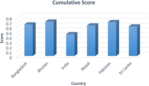
Table 9 presents the outcomes of the T.O.P.S.I.S. method for the performance of underline indicators in South Asian economies. The performance of these indicators is improving after 2005 in Bangladesh. Bhutan is facing the issue of fluctuation in these indicators’ performance during the estimated period. For example, it attained a 0.86 score in 2000 while closed 2020 with 0.76. India’s performance looks consistently poor throughout the given period as it achieves only 0.5 scores on average. The indicators performance of Nepal, Pakistan, and Sri Lanka always show positive and improving throughout the period. Therefore, T.O.P.S.I.S. results are very optimistic regarding the performance of underline indicators in South Asia except for India.

According to the outcomes of the T.O.P.S.I.S. method presented in Figure 1, the cumulative results of Bhutan’s performance are highly optimised among the underlying countries as she attained the highest (0.71) score. These results indicate that Bhutan’s H.C. strategy supports E.P., inflation, carbon emission, and taxation. In this analysis, Pakistan is the second-best performing country with 0.70 scores, followed by Bangladesh (0.65). Based on the underlying indicators, India’s performance has worsened much, and it has attained the lowest score (0.45) in this lineup. Thus, results indicate that H.C. in India suffers a lot due to carbon emission, E.P., inflation, and taxation. These results also support the regression outcomes that E.P., carbon emissions, P.C.I., and inflation are the leading sources of stress H.C. in the South Asian region.

Figure 1. Cumulative score of South Asian based on T.O.P.S.I.S.

Authors calculations based on STATA.

4. Discussion

This study applied two distinguished research methods to probe the relationship between H.C. and policy mix (tax and inflation), E.P., carbon emission, and economic growth. According to the F.E. model of econometrics, E.P. has a substantial and positive impact on H.C. in the South Asian region. This result indicates that higher E.P. in the area may affect the H.C. pattern. The same results were generated by Moshiri (2015) and Sarkodie et al. (2020) that demand's overall energy price elasticities are small, but income elasticities are close to one. Thus, households show a more robust response to energy price changes. Consequently, the results show that the region's present energy price rise policy will not exclusively reduce energy usage but negatively impact H.C. patterns for other necessary commodities. Because of this, the price of energy is set at levels that are far above what people require (Zou et al., 2020). These outcomes regarding E.P. are highly significant under the P.Q.R. method.

Policy mix instruments (taxation and inflation) have a significant impact on H.C. in South Asia. The increase of the rate of tax or inflation is a source of high H.C. In F.E. model estimations, I.N.F. is a source of high H.C. while tax rate (T.A.X.) reduces the power of purchase of individual consumers. The relationship between H.C. and the tax rate was established by Ortigueira and Siassi (2021) and endorsed by Goncharuk and Cirella (2020) and Adedoyin et al. (2020) based on commodity taxes like energy tax.

The cost of environmental degradation due to carbon emission is very high in H.C. Carbon emission may increase the health expenditure in the H.C. pattern. Early research also endorsed the notion in this regard. For example, Zhang et al. (2017) found that CO₂ emission is a source of H.C. accumulation, while Feng et al. (2011) estimated that CO₂ emissions increase faster than the direct consumption values. Thus, the impact of environmental degradation on household income is enormous. According to the P.Q.R. outcomes, carbon emission is a continuous H.C. accelerator throughout all quantiles.

Finally, this study utilised the P.C.I. variable as an independent variable to verify that higher-income induces higher H.C. This variable is also a test case of the model in line with the Keynesian consumption theory (Tanrikulu, 2021). Our model verified this notion that income and H.C. have positive relationships in the long run.

The T.O.P.S.I.S. outcomes of operational results highlight the performance of all indicators in an individual country. According to its outcomes, Bhutan has the best performance in the given hands, followed by Pakistan and Bangladesh, while India's performance in this regard is abysmal and needs special intentions.

5. Conclusions and policy implications

This study utilised 31 years’ data set of six South Asian countries to determine the relationship between human capital and E.P., carbon emission, policy mix tools. Furthermore, this study attempted to empirically analyse the Keynesian consumption theory for the South Asian region. For this purpose, this study used F.E. model, and P.Q.R. tools from econometric and T.O.P.S.I.S. techniques from operational research. Both the methods confirm the relationship between the underline factors. The policy mix instruments (I.N.F. and T.A.X.) are the leading H.C. patterns in these economies. Inflation increases the level of H.C. due to pursuing fewer commodities against the local currency. At the same time, the tax rate reduces the power of purchase of the consumer and leaves fever money for commodities.

E.P. also has a positive share in H.C. It indicates that H.C. surge due to increased E.P. in the local and international markets. This notion is logically supported as the economies of South Asia are highly dependent on import-based energy. Finally, the relationship between carbon emission and H.C. has been found positive. It indicates that environmental degradation increases pressure on H.C. These results are verified through P.Q.R. The variables mentioned above show the continuous impact on H.C. during the study period with minor fluctuations.

Finally, the results of indicators performance based on T.O.P.S.I.S. (an operational research method) show that all these indicators in underline countries are not up to the mark. However, Bhutan attained the highest performance position, while Pakistan and Bangladesh are the second and third best countries. India’s performance among underline countries in these indicators has worsened, followed by Sri Lanka and Nepal.

Based on this empirical evidence, H.C. is compassionate against E.P., carbon emission, and policy mix instruments. Therefore, a policy review is deemed required in these three sides of the economy.

• In the current world scenario, green and clean energy initiatives have a combo impact on energy supply, E.P., and control of carbon emission. Renewable energies could be used to meet the country's home energy needs instead of traditional fossil fuels for this multi-purpose project. South Asia needs to initiate green and clean energy projects.

• A separate green energy financing may help them replace their old, outdated, expensive, carbonised, and inefficient energy system with a clean, carbon-free, and efficient energy supply.

• The policy mix tools should be applied with considering their relationship with H.C. The rate of tax and inflation need to be stable over time. For this purpose, macroeconomic indicators and monetary instruments need to be used carefully.

Disclosure statement

No potential conflict of interest was reported by the authors.

Additional information

Funding

National Natural Science Foundation of China (No.72103054); China Postdoctoral Science Foundation (No. 2021T140181); Ministry of education, humanities, and social sciences research projects (No. 19YJA790121).

References

- Abbas, Q., Nurunnabi, M., Alfakhri, Y., Khan, W., Hussain, A., & Iqbal, W. (2020). The role of fixed capital formation, renewable and non-renewable energy in economic growth and carbon emission: A case study of Belt and Road Initiative project. Environmental Science and Pollution Research International, 27(36), 45476–45486. https://doi.org/10.1007/s11356-020-10413-y
- Adedoyin, F., Ozturk, I., Abubakar, I., Kumeka, T., Folarin, O., & Bekun, F. V. (2020). Structural breaks in CO2 emissions: Are they caused by climate change protests or other factors? Journal of Environmental Management, 266, 110628. https://doi.org/10.1016/j.jenvman.2020.110628
- Al Mamun, M., Sohag, K., Hannan Mia, M. A., Salah Uddin, G., & Ozturk, I. (2014). Regional differences in the dynamic linkage between CO2 emissions, sectoral output and economic growth. Renewable and Sustainable Energy Reviews, 38(C), 1–11. https://doi.org/10.1016/j.rser.2014.05.091
- Alexander, M., Harding, M., & Lamarche, C. (2011). Quantifying the impact of economic crises on infant mortality in advanced economies. Applied Economics, 43(24), 3313–3323. https://doi.org/10.1080/00036840903559620
- Ali, I., Shafiullah, G. M., & Urmee, T. (2018). A preliminary feasibility of roof-mounted solar PV systems in the Maldives. Renewable and Sustainable Energy Reviews, 83, 18–32. https://doi.org/10.1016/j.rser.2017.10.019
- Bai, J., & Ng, S. (2005). Test for skewness, kurtosis and normality for time series data. Journal of Business & Economic Statistics, 23(1), 49–60. https://doi.org/10.1198/073500104000000271
- Ben Rejeb, A. (2017). On the volatility spillover between Islamic and conventional stock markets: A quantile regression analysis. Research in International Business and Finance, 42, 794–815. https://doi.org/10.1016/j.ribaf.2017.07.017
- Cantore, C., & Freund, L. B. (2021). Workers, capitalists, and the government: Fiscal policy and income (re)distribution. Journal of Monetary Economics, 119, 58–74. https://doi.org/10.1016/j.jmoneco.2021.01.004
- Chan, Y. T. (2020). Are macroeconomic policies better in curbing air pollution than environmental policies? A DSGE approach with carbon-dependent fiscal and monetary policies. Energy Policy, 141, 111454. https://doi.org/10.1016/j.enpol.2020.111454
- Diawuo, F. A., Scott, I. J., Baptista, P. C., & Silva, C. A. (2020). Assessing the costs of contributing to climate change targets in sub-Saharan Africa: The case of the Ghanaian electricity system. Energy for Sustainable Development, 57, 32–47. https://doi.org/10.1016/j.esd.2020.05.001
- Fang, Z., & Chang, Y. (2016). Energy, human capital and economic growth in Asia Pacific countries – Evidence from a panel cointegration and causality analysis. Energy Economics, 56(c), 177–184. https://doi.org/10.1016/j.eneco.2016.03.020
- Feng, Z. H., Zou, L. L., & Wei, Y. M. (2011). The impact of household consumption on energy use and CO2 emissions in China. Energy, 36(1), 656–670. https://doi.org/10.1016/j.energy.2010.09.049
- Ghorbani, A., Rahimpour, M. R., Ghasemi, Y., & Raeissi, S. (2018). The biodiesel of microalgae as a solution for diesel demand in Iran. Energies, 11(4), 950. https://doi.org/10.3390/en11040950
- Goncharuk, A. G., & Cirella, G. T. (2020). A perspective on household natural gas consumption in Ukraine. The Extractive Industries and Society, 7(2), 587–592. https://doi.org/10.1016/j.exis.2020.03.016
- Halbac-Cotoara-Zamfir, R., Smiraglia, D., Quaranta, G., Salvia, R., Salvati, L., & Giménez-Morera, A. (2020). Land degradation and mitigation policies in the mediterranean region: A brief commentary. Sustainability, 12(20), 8313. https://doi.org/10.3390/su12208313
- Halff, A., Younes, L., & Boersma, T. (2019). The likely implications of the new IMO standards on the shipping industry. Energy Policy, 126, 277–286. https://doi.org/10.1016/j.enpol.2018.11.033
- Harris, D., Leybourne, S., & McCabe, B. (2005). Panel stationarity tests for purchasing power parity with cross-sectional dependence. Journal of Business & Economic Statistics, 23(4), 395–409. https://doi.org/10.1198/073500105000000090
- Im, K. S., Pesaran, M. H., & Shin, Y. (2003). Testing for unit roots in heterogeneous panels. Journal of Econometrics, 115(1), 53–74. https://doi.org/10.1016/S0304-4076(03)00092-7
- Iqbal, W., Fatima, A., Yumei, H., Abbas, Q., & Iram, R. (2020). Oil supply risk and affecting parameters associated with oil supplementation and disruption. Journal of Cleaner Production, 255, 120187. https://doi.org/10.1016/j.jclepro.2020.120187
- Koenker, R. (2004). Quantile regression for longitudinal data. Journal of Multivariate Analysis, 91(1), 74–89. https://doi.org/10.1016/j.jmva.2004.05.006
- Koenker, R. (2017). Quantile regression: 40 years on. Annual Review of Economics, 9(1), 155–176. https://doi.org/10.1146/annurev-economics-063016-103651
- Koenker, R., & Bassett, G. (1978). Regression quantiles. Econometrica, 46(1), 33–50. https://doi.org/10.2307/1913643
- Moshiri, S. (2015). The effects of the energy price reform on households consumption in Iran. Energy Policy, 79(C), 177–188. https://doi.org/10.1016/j.enpol.2015.01.012
- Murad, M. W., Alam, M. M., Noman, A. H. M., & Ozturk, I. (2019). Dynamics of technological innovation, energy consumption, energy price and economic growth in Denmark. Environmental Progress & Sustainable Energy, 38(1), 22–29. https://doi.org/10.1002/ep.12905
- Natalini, D., Bravo, G., & Newman, E. (2020). Fuel riots: Definition, evidence and policy implications for a new type of energy-related conflict. Energy Policy, 147, 111885. https://doi.org/10.1016/j.enpol.2020.111885
- Notarnicola, B., Tassielli, G., Renzulli, P. A., & Monforti, F. (2017). Energy flows and greenhouses gases of EU (European Union) national breads using an LCA (Life Cycle Assessment) approach. Journal of Cleaner Production, 140(2), 455–469. https://doi.org/10.1016/j.jclepro.2016.05.150
- Omojolaibi, J. A., & Egwaikhide, F. O. (2014). Oil price volatility, fiscal policy and economic growth: A panel vector autoregressive (PVAR) analysis of some selected oil-exporting African countries. OPEC Energy Review, 38(2), 127–148. https://doi.org/10.1111/opec.12018
- Ortigueira, S., & Siassi, N. (2021). The U.S. tax-transfer system and low-income households: Savings, labor supply, and household formation. Review of Economics Dynamic, 44, 184–210. https://doi.org/10.1016/j.red.2021.02.010
- Rasaq Adejumobi, A., & Olatunde Julius, O. (2017). Oil price shocks and foreign direct investment (FDI): Implications for economic growth in Nigeria (1980-2014). Journal of Economics and Sustainable Development, 8(4), 170–177.
- Rekha Manjunath, S., Sivarajadhanavel, P., & Krishnamoorthy, V. (2020). Foreign currency such as US dollar, Euro, pound sterling, Japanese Yen, gold and crude oil price impact on Indian stock indices – BSE and NSE. International Journal of Scientific & Technology Research, 9(3), 6809–6817.
- Sarkodie, S. A., Adams, S., Owusu, P. A., Leirvik, T., & Ozturk, I. (2020). Mitigating degradation and emissions in China: The role of environmental sustainability, human capital and renewable energy. The Science of the Total Environment, 719, 137530. https://doi.org/10.1016/j.scitotenv.2020.137530
- Sun, H., Khan, A. R., Bashir, A., Alemzero, D. A., Abbas, Q., & Abudu, H. (2020). Energy insecurity, pollution mitigation, and renewable energy integration: Prospective of wind energy in Ghana. Environmental Science and Pollution Research International, 27(30), 38259–38275. https://doi.org/10.1007/s11356-020-09709-w
- Tang, C. F., Yip, C. Y., & Ozturk, I. (2014). The determinants of foreign direct investment in Malaysia: A case for electrical and electronic industry. Economic Modelling, 43, 287–292. https://doi.org/10.1016/j.econmod.2014.08.017
- Tanrikulu, C. (2021). Theory of consumption values in consumer behaviour research: A review and future research agenda. International Journal of Consumer Studies, 45(6), 1176–1197. https://doi.org/10.1111/ijcs.12687
- Warr, B., & Ayres, R. U. (2012). Useful work and information as drivers of economic growth. Ecological Economics, 73, 93–102. https://doi.org/10.1016/j.ecolecon.2011.09.006
- Yeh, S., Burtraw, D., Sterner, T., & Greene, D. (2021). Tradable performance standards in the transportation sector. Energy Economics, 102, 105490. https://doi.org/10.1016/j.eneco.2021.105490
- Zhang, Y. J., Bian, X. J., Tan, W., & Song, J. (2017). The indirect energy consumption and CO2 emission caused by household consumption in China: An analysis based on the input–output method. Journal of Cleaner Production, 163, 69–83. https://doi.org/10.1016/j.jclepro.2015.08.044
- Zou, H., Luan, B., Zheng, X., & Huang, J. (2020). The effect of increasing block pricing on urban households’ electricity consumption: Evidence from difference-in-differences models. Journal of Cleaner Production, 257, 120498. https://doi.org/10.1016/j.jclepro.2020.120498