Implementation of standards into predictors of financial stability

Abstract

This article proposes a methodology for modifying bankruptcy models. The authors focused on the role of partial predictors in predicting companýs bankruptcy. According to the authors, it is necessary to analyse the anomalies that occur in companies that are losing financial stability. It has been hypothesized that some anomalies in the form of extreme values ​​may deviate the overall final value of the model to such an extent that they lead to an erroneous evaluation of the company by the bankruptcy model. As a result, companies in bankruptcy may be incorrectly classified as 'financially stable' or, conversely, financially sound companies with certain extreme values ​​could be mistaken for companies in bankruptcy. To verify the hypothesis, the authors analysed the probability distribution of partial predictors of the bankruptcy Model 1 on a test and verification sample of more than 1,100 companies. Limits were set to eliminate extreme values ​​and, as a result, the accuracy of the model has been increased. The introduction of limits has increased the accuracy of the model, especially in ​​bankruptcy prediction. For bankruptcies, the accuracy increased from 85.82% to 88.65% for the test sample and from 84.00% to 88.00% for the verification sample.

Keywords:

• Economic development
• financial stability
• bankruptcy model
• outliers

JEL CLASSIFICATIONS:

• M21
• G01
• G32
• C53

1. Introduction

Bankruptcy models were created for the purpose of quick and easy company rating. Their creation and development dates back to the time when Professor Altman created and popularized his Z-score in 1968 (Altman, 1968). He was followed by a number of experts with their own bankruptcy prediction models (e.g., Ohlson, 1980; Zavgren, 1985; Shumway, 2001; Ahn & Kim, 2009; Li et al., 2011).

The vast majority of these models usually try to answer the question of current financial health using a weighted average of selected predictors. Predictors usually take the form of financial ratios that can eliminate the effect of business size to ensure that the model is applicable to all businesses. These ratios vary from model to model. These are usually tools used in financial analysis in the field of measuring profitability, liquidity, indebtedness, and activity of the company - or their modifications (see e.g. Ajaz et al., 2019; Blazkova & Dvoulety, 2018; Voda et al., 2021; Kovacova et al., 2019). However, these ratios do not evaluate the company comprehensively. Therefore, these financial ratios are supplemented by a selected bankruptcy model or other comprehensive indicator (e.g. Belas et al., 2020; Prodanova et al., 2019).

The input values ​​of these indicators are accounting data. The recommended values ​​of these financial indicators are set for a normal or financially sound company. Sometimes, however, the book values deviate from normal, especially in bankrupt companies. To a certain extent, this is precisely the characteristic of a bankrupt company, on the basis of which the model designates it as bankrupt. But standard financial analysis indicators do not take into account that several extreme values ​​could occur within one ratio. Given that traditional bankruptcy models are also designed for the lay user, such a user of the model cannot be expected to evaluate one or more predictors that are part of the bankruptcy model as erroneous values ​​that do not correspond to reality, due to the combination of several extreme values. Such an extreme may subsequently deviate the overall rating and the ability of the model to correctly classify the company as bankrupt or non-bankrupt. In the opinion of the authors, these are mainly cases where the state of inventories or other assets is minimized due to a malfunction of the company, a negative value of equity, indebtedness above 100%, or zero value of certain accounting items.

In the past there have been various ways how to improve the model accuracy. For example, focus on a specific region, business size, manufacturing/services, industry, or specific product. Various statistical methods are tested and qualitative predictors or macroeconomic variables with different success rates are also implemented in the models. It is usually a combination of several of these options in parallel.

However, no expert has yet dealt with a deeper analysis of unwanted anomalies. So far, all studies have focused only on the elimination of outliers in data samples, which were then to be used in creating a bankruptcy model. Therefore, this empirical research focused on the analysis of outliers in the companies to which the model is applied.

The study is constructed in the following way. In the first section is presented introduction. In second section is the literature review. In third section is aim, sample of data and methodology description. In the fourth are research results. The last part includes conclusion.

2. Literature review

Not all models are specialised in companies based on the branch, the specific business activity or company size. Gupta et al. (2018) analysed the diversity between micro, small, and medium-sized companies while predicting bankruptcy and financial distress. He found that survival (failure) probability increases (decreases) with increasing company size and companies in different size categories have varying determinants of bankruptcy, whereas factors affecting their financial distress are mostly invariant. Given that this information provides a source of information for the development of quantitative predictors, the logical deduction is that the industry factor may have an impact on the model's predictive power. And studies confirm the impact of the industry (e.g. Pech et al., 2020). For example, company size and industry classification factors were taken into account by Slavicek and Kubenka (2016), who suggested their own prediction model for small companies in the construction industry called Model 1. The impact awareness of the size and industry of a company on the model's predictive power existed much earlier, but many authors did not take these factors into account in the development of their models, for example (Jiang & Jones, 2018; Christopoulos et al., 2019). The impact of the industry and size in certain specific cases has already been proved. For this reason, we are in favour of the need to create models directly for a particular size category of companies and a specific industry or closely related industries despite the fact that this in turn reduces their applicability. Also, the company's management 'records' can be maintained in different accounting systems which affects the structure of financial data as well as the value of accounting items (Mousavi et al., 2019; Jabeur, 2017; Charalambous et al., 2020). Most of these model makers are firmly convinced that each region is so specific that its own local model should be developed. On the contrary, Alaminos et al. (2016) claim that their global model is more accurate in comparison to regional models over three years prior to bankruptcy. Other multiregional models were developed by Eling and Jia (2018), Jones (2017), or Jones and Wang (2019). In light of the above, we believe that a degree of influence of the model’s regional focus on its accuracy should be considered. Historically, model makers analysed what source information should be included in predictors to maximize their predictive power. They also addressed the question what role source quantitative and qualitative information play in the success of predictors. The existing predictors contain quantitative, qualitative or a combination of this information. Key quantitative factors of financial stability usually include cash flow, liquidity, profitability, leverage and another financial data from account data included in financial statements (Alaka et al., 2017). The accounting data is created in accordance with the established rules of accounting systems based on the legislation of the given country or region. It ensures that data is systematic and consistently created for the given region. However, accounting systems show certain differences (Honkova, 2015). Key qualitative factors are undoubtedly management characteristics, owners, internal strategy, and macroeconomic environment. The assessment of these and other qualitative factors may sketch the actual financial position of the company and may help to predict the future development, including on-coming insolvency more accurately. Against it Bao et al. (2020) draw attention to a danger related to a purposeful falsification of information provided by managers when they strive to present mainly positive aspects of the company activities. Another problem is the availability of such qualitative data.

The vast majority of prediction models use quantitative data from corporate accounting systems or financial markets with clearly prevailing accounting data in information sources (see e.g. Jones, 2017). Just a small number of models have recently started to include macroeconomic data from the external environment in their predictors. For example, Vo et al. (2019) said that 'The empirical findings confirm that the corporate financial distress prediction model, which includes accounting factors with macroeconomic indicators, performs much better than alternative models.' This is also confirmed by Bhattacharjee and Han (2014), Zikovic (2016) and Tinoco et al. (2018). Many model makers reviewed the accuracy of prediction in a period of several years before bankruptcy. In most cases, they tried to quantify how much the model's predictive power was reduced 1 to 5 years before bankruptcy. The results show that as the number of years preceding bankruptcy increases, the accuracy of the model decreases (see e.g. Karas & Režňáková, 2017; Jabeur, 2017). A more recent idea is to​​ include more periods in the model to reflect the dynamics of changes in input variables. Kim and Partington (2015) and Jones (2017) studied the accounting and financial market data. Their research shows and they claim that a dynamic model incorporating a period of the last two or more years is more accurate than the static model.

Experts have been looking at different ways to improve the models accuracy. They often eliminate outliers in business samples before creating new models. But what if the model encounters an outlier when it is applied to a specific business later?

Efforts have been made in the past to examine the relationship between the occurrence of outliers and the models´ accuracy. Certainly, methods where values are categorized (e.g. CART, CHAID or Tamari's, 1966 Risk Index ) efficiently, deal with this problem. However, most other models do not solve this problem.

For example, McLeay and Azmi (2000) examined the effect of outliers on MDA-based models and on logistic regression. It turned out that outliers really reduce the models´ accuracy. They also proposed solutions to eliminate the impact of outliers.

Linares-Mustaros et al. (2018) put forward an alternative financial statement analysis method for classifying firms which aims at solving skewed distributions, outliers, and redundancy and draws from compositional data analysis. The method is based on the use of the existing clustering methods with standard software on transformed data by means of the so-called isometric logarithms of ratios.

Yang et al. (2004) propose a novel "two-phase" support vector regression training algorithm to detect outliers and reduce their negative impact. Their experimental results has improvement on the prediction.

Nyitrai and Virag (2019) propose the CHAID-based categorization of financial ratios as an effective way of handling outliers with respect to the predictive performance of bankruptcy prediction models.

Other examples of how to mitigate or eliminate the impact of outliers can be found. However, the authors of this article base their research on the requirements of bankruptcy models, which is, among other things, the speed of calculation and user friendliness guaranteeing that the model can be used by a lay person. Therefore, the authors of this article focused on the improvement of a model accuracy while maintaining simplicity in its application.

3. Aim, data and methodology

3.1. Aim of the research

The authors are not aware of the case of the bankruptcy model, which would focus its attention on remote values ​​only when applying the model. The authors are convinced that so far no expert has addressed the influence of negative combinations of outliers in predictors of financial distress. Therefore, this research addresses this problem in order to find another way to increase the accuracy of existing bankruptcy models. To this end, two hypotheses were introduced:

H1: Partial predictors of the selected bankruptcy model, when applied to a data sample, also show outliers.

H2: Reducing outliers of partial predictors can improve the predictive power of a selected bankruptcy model.

The aim of the research is to eliminate undesirable anomalies of partial predictors and, as a result, to increase the accuracy of the selected bankruptcy model.

3.2. Data

The survey works with four representative sets of companies, which were created by random sampling. A test sample and a verification sample were created from small companies operating in the Czech Republic in the construction industry, which contains accounting data of each company in the last five years, i.e. from 2014 to 2018. The test sample contains a set of non-bankrupt companies with data for the last 5 years and a set of companies which went bankrupt, also 1 year (t-1) to 5 years (t-5) before their bankruptcy in 2019. Predictor limits will be applied to this sample in order to eliminate extremes which, in the authors' opinion, reduce the predictive power of the tested Model 1. The verification sample also includes a set of bankruptcy companies as well as a set of non-bankruptcy companies. It will then prove or disprove whether the limits found can be successfully applied to other companies in order to achieve better predictive power of the Model 1. The test sample contains 752 companies and the verification sample 415 companies. Their structure is shown in Figure 1 and Table 1. Data were gathered from The Bisnode’s MagnusWeb (2020) database (www.magnusweb.cz).

Figure 1. Samples of data.

Source: Own processing

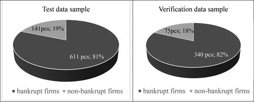
Table 1. Description of samples from Figure 1.

Sample	Average Assets	Average Short-term assets	Average Sales	Average Earnings after taxes	Legal form
					JSC	Ltd.
141 pcs	15609	7906	23898	−2811	1	140
611 pcs	91493	46961	126960	5960	17	594
75 pcs	16195	9321	22424	−5176	0	75
340 pcs	95942	54335	125792	6137	13	327

Note: JSC means “a joint stock company”, Ltd. means “a limited company”, conversion of CZK to EUR according to the exchange rate of the Czech National Bank (25.643 CZK/EUR).

Source: Author´s calculations.

Samples has been selected on the random basis. None of the companies in the set of non-bankrupt companies showed signs of bankruptcy in the form of insolvency or negative equity (the same methodology as Kubenka, 2018) in this case from 2014 to 2018 and one year later (2019). Set of bankrupt companies includes also financial statements according to Czech Accounting Standards. These companies went bankrupt in 2019 according to Act No. 182/2006 Coll., on Insolvency, as amended in Czech law.

3.3. Model used

A bankruptcy model was chosen which has a clear and publicly available structure and a sufficiently described creation methodology, and also met the following criteria:

• novelty,

• focus on a specific sector (the model used is focused on construction),

• high accuracy of the model,

• availability of accounting data of companies created on the same accounting basis as the accounting data used to create the model (these are Czech Accounting Standards for Entities Accounting under Regulation no. 500/2002, according to Act No 563/1991 Coll., on Accounting).

For example, models created using neural networks do not meet such requirements. The model from the authors Slavicek & Kubenka from 2016, which the authors call Model 1, meet the requirements. The model was created on the basis of logit regression on a sample of 22 non-bankrupt and 11 bankrupt companies from the construction sector.

The M1 component is a combination of financial ratios and weights of importance and contains one constant. The financial ratios in Table 2 (ITR, CR1, ROA, TIR) are multiplied by the weights of importance W1 (0.0173), W2 (−4.7107), W3 (−0.0412), W4 (0.0918), as indicated the following functions (1). (1) $$\text{M1 component }=0.0\text{173IT }-\text{4}.\text{71}0\text{7L1 }–0.0\text{412ROA }+0.0\text{918TIR }–\text{7}.\text{5378}$$(1)

Table 2. Indicators used to calculate the M1 component* included in model 1.

Group of Ratios	Indicator	Enumeration
Turnover ratios	ITR – Inventory Turnover	$\frac{360\text{ x inventory}}{\mathrm{revenues}}$
Liquidity ratios	CR1 – Liquidity 1	$\frac{\mathrm{short}-\text{term financial property}}{\mathrm{short}-\text{term liabilities}}$
Activity ratios	ROA – Return on Assets	$\frac{\text{operating profit}}{\text{total asset}}$
Debt ratios	TIR – Total Debt Ratio	$\frac{\text{total debt}}{\text{total asset}}$

Note: The authors tried to use other components when creating the model. The component in this article, designated M1 component, was rated as the best to maximize model accuracy.

Source: composed by the authors based on Slavicek and Kubenka (2016).

Model 1 draws input data from the accounting records of the company, which is assessed by this bankruptcy model. This is financial information about the company recorded in the balance sheet and profit/loss statement. Using this model, the company is classified as either a bankrupt firm (for $\pi$ > 0.5) or a non-bankrupt firm (for $\pi$ <0.5) according to the following formula (2). (2) $$\pi =\frac{e^{M1}}{1+\mathrm{ }{e}^{M1}}$$(2)

3.4. Expression of model accuracy

The following method was chosen to express the accuracy of the model, because it expresses separately the accuracy in the classification of bankruptcy and separately the accuracy in estimating non-bankruptcy. The success rate of bankruptcy prediction for the financially unstable enterprises will be hereinafter referred to as sensitivity also called true positive rate (TPR) and expressed as a percentage. This share indicator has the following form: (3) $$\mathit{TPR}=\frac{\text{True I}.}{\text{True I}.\mathrm{ }+\text{Error I}.}$$(3)

'True I. 'values and 'Error I.' in formula (3) are the numbers of bankruptcy companies that were correctly and incorrectly classified according to classification matrix (Table 3). TNR will be used for the true negative rate also called specificity. The resulting value is also expressed as a percentage. For most models, specificity > sensitivity, the respective success rate of the company's financial stability prediction (non-bankrupt) is higher than the success rate of bankruptcy prediction. Formula (4) expresses the method of calculating the TNR. (4) $$\mathit{TNR}=\frac{\text{True II}.}{\text{Error II}.\mathrm{ }+\text{True II}.}$$(4)

Table 3. Classification matrix.

		Prediction
		Bankrupt	Non-bankrupt
Fact	Bankrupt	True I.	Error I.
	Non-bankrupt	Error II.	True II.

Source: created by the authors based on Kubenka and Myskova (2019).

Then the total success rate (TSR) of a concrete model can be calculated as an arithmetical average of TPR and TNR as follows. (5) $$\mathit{TSR}=\frac{\mathrm{TPR}+\mathrm{TNR}}{2}$$(5)

3.5. Wilcoxon signed-rank test

This non-parametric test is used to compare two related samples, in our case repeated measurements, on a single sample to assess whether their means differ. That is the answer to the question of whether two analysed samples were selected from populations having the same distribution.

Lowry (2020) states that the Wilcoxon test makes certain assumptions and can be meaningfully applied only insofar as these assumptions are met. Namely, that the scale of measurement for sample 1 and sample 2 has the properties of an equal-interval scale, that the differences between the paired values of sample 1 and sample 2 have been randomly drawn from the source population, and that the source population from which these differences have been drawn can be reasonably supposed to have a normal distribution.

The null hypothesis of the Wilcoxon signed rank is the same as the sign test (Mendenhall et al., 1990), i.e. both tests test hypothesis about the median. A complete description of methodology of Wilcoxon signed-rank test is given, for example, in Akeyede et al. (2014).

3.6. Grubbs’ test for outliers detection

Grubbs's test is based on the assumption of normality. However, this test will be used with reference to the central limit theorem because the data files are large and the probability distribution is close to the normal distribution. After sorting the data points from smallest to largest, we find the mean (x̄) and standard deviation of the data set. G test statistic for a two-tailed test uses the following equations: (6) $$\mathrm{G}\mathrm{ }=\mathrm{ }\frac{\underset{i=1,.N}{\max }\left|Yi-\mathrm{Ȳ}\right|}{s}$$(6) where ȳ is the sample mean,s = sample standard deviation.

G critical values we can find in tables or manually we can find the G critical value with a formula: (7) $$G>\frac{N-1}{\sqrt{N}}\sqrt{\frac{t_{\alpha /(2N),N-2}^2}{N-2+t_{\alpha /(2N),N-2}^2}}$$(7) where t_{α/(2N),N−2} is the upper critical value of a t-distribution with N-2 degrees of freedom.

If we compare G test statistic to the G critical value and G_test > G_critical, then we should reject the point as an outlier. We should keep the point in the data set if

G_test < G_critical because it is not an outlier.

4. Research results and discussion

Model 1 was applied to sample 1 (611 non-bankrupt, 141 bankrupt). The resulting values of M1 components are graphically shown in Figure 2. The median and quantiles of 25% −75% in non-bankrupt enterprises (in Figure 2 market as “NON”) show relatively stable values.

Figure 2. Box plots of non-bankrupt (NON) firms and bankrupt (BAN) firms.

Source: Author´s calculations

For companies in bankruptcy, we can observe changes in median values towards positive values. Also, the 25% quantile and much more the 75% quantile increase their deviation from the median and increase their value.

Wilcoxon signed-rank test proved with statistical significance that the M1 component index changed 2 years before the bankruptcy of bankrupt companies (that is, between years t-2 and t-3, and years t-1 and t-2). In previous years, the Wilcoxon test did not prove this in bankruptcy companies (i.e. year-on-year between years t-5 and t-4 and between years t-4 and t-3). For non-bankrupt companies, the Wilcoxon test did not show a statistically significant year-on-year change in M1 component in any year in the entire period under review for five consecutive years.

Based on these facts, the success of the model (TNR or TPR) was monitored 3 years before the bankruptcy or non-bankruptcy, including basic characteristics of M1 components. It is clear that companies that are heading for bankruptcy are starting to show negative symptoms several years before bankruptcy. This is reflected in the growth of the M1 components (median) index, the growth of which should point to the impending bankruptcy.

It is clear from Table 4 that the accuracy of the prediction of financial health in years is relatively stable for non-bankrupt enterprises and TNR values range from 88.54 to 89.85% with an upward trend in TNR growth. In contrast, Table 5 shows that the economic situation of bankruptcy companies is deteriorating gradually, and the closer the company is to its bankruptcy, the more negative symptoms manifest. This is proved by the increase of accuracy (TPR) between the years t-3 and t-1 by about 30%. In addition to the widening of the gap between the quantiles and the median of M1 components in the last year, bankruptcy companies are also experiencing an extreme increase in the standard deviation.

Table 4. TNR of Model 1 and statistical values of M1 components in non-bankrupt enterprises.

t	n	No. of π < 0.5	Accuracy (TNR)	MeanM1	MedianM1	MinM1	MaxM1	Q1M1	Q3M1	SDM1
t-3	611	541	88.54%	−4.054	−3.015	−57.392	15.546	−5.552	−1.039	5.805
t-2	611	545	89.20%	−4.216	−2.981	−81.646	19.453	−5.498	−1.003	6.544
t-1	611	549	89.85%	−4.521	−3.201	−73.597	21.899	−5.778	−1.038	6.601

Source: Author´s calculations.

Table 5. TPR of model 1 and statistical values of M1 components in bankrupt enterprises.

t	N	No. of π > 0.5	Accuracy (TPR)	MeanM1	MedianM1	MinM1	MaxM1	Q1M1	Q3M1	SDM1
t-3	141	79	56.03%	0.650	0.933	−17.816	15.184	−0.836	2.578	5.100
t-2	141	93	65.96%	2.660	1.291	−22.273	17.329	−0.065	5.558	6.625
t-1	141	121	85.82%	7.262	4.887	−56.794	47.703	1.365	13.024	14.251

Source: Author´s calculations.

The authors assume that the inaccuracy of the prediction when using the Model 1 with M1 component is partly caused by the occurrence of extreme values in the partial predictors (ITR, CR1, ROA, TIR). In general, we could divide these extreme values into two categories:

1. desired deviations - these are those that indicate a negative development,

2. undesirable deviations - these are those that indicate a negative development, but thus reach high/low values that they may undermine the basic principles of the operation of ratio indicatiors.

To verify H1¹, the distribution of the values of the partial predictors will be graphically assessed.

The spot graph of ITR, CR1, ROA, TIR in figure 3 shows that this is not a normal distribution. The graphs visually show that outliers exist for the ITR, CR1, ROA and TIR predictors. Therefore, a Grubbs´s test of outliers was applied to the sets of predictors of bankruptcy and non-bankruptcy companies from 2018. This test also confirmed the existence of outliers. As expected, the outliers test showed that for none of the sub-predictors did the number of outliers exceed 1% of the largest or smallest values. Therefore, limits were set at the .01 percentile for the smallest of the values of the ITR, CR1, ROA, TIR sub-predictors and at the .99 percentile for the highest values.

Figure 3. Spot graph of ITR, CR1, ROA, TIR in 2018.

Source: Own processing

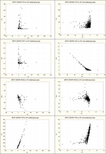
Tables 6 and 7 show that the statistics of the partial predictors of bankruptcy and non-bankruptcy enterprises in some cases even overlap in the achieved values.

Table 6. Percentiles 0.01 and 0.99 of non-bankrupt enterprises in M1 component.

	n	Mean	Median	Min	Max	Q1	Q3	Perc. .01	Perc. .99
ITR	611	55.430	46.218	0.000	1255.816	25.393	71.001	2.466	199.568
CR1	611	0.417	0.083	−0.249	14.311	0.020	0.281	0.0002	5.894
ROA	611	6.002	4.478	−36.831	87.240	0.879	9.920	−18.166	37.683
TIR	611	47.502	46.898	3.158	99.641	29.014	64.752	7.476	94.507
M1	611	−4.431	−3.077	−73.597	21.900	−5.758	−0.931	−33.503	2.290

Notes: ITR - Inventory Turnover Ratio. CR1–Liquidity 1. ROA: Return on Assets; TIR: Total Debt Ratio. Source: Author´s calculations.

Table 7. Percentiles 0.01 and 0.99 bankruptcies.

	n	Mean	Median	Min	Max	Q1	Q3	Perc. .01	Perc. .99
ITR	141	105.240	12.683	0	2794.076	0	57.052	0	2794.076
CR1	141	0.07655	0.0153	−0.18056	1.93415	0.00357	0.05568	−0.17535	0.66049
ROA	141	−155.972	−23.752	−16608.826	26.959	−57.142	−5.040	−227.649	26.629
TIR	141	354.311	126.320	33.856	24556.062	91.892	218.179	34.503	1572.131
M1	141	32.874	5.886	−11.786	2930.990	1.564	16.231	−5.397	138.607

Source: Author´s calculations.

However, when using the Model 1, the analyst will not know whether he is testing a company that will go bankrupt in the future or will be financially stable. This is regardless of the achieved $\pi$ value, because the model does not have an accuracy of 100%. Therefore, the .01 and 0.99 percentiles of predictors in M1 component need to be determined for the entire test sample, which is a total of 752 bankrupt and non-bankrupt companies. Percentiles 0.01 and 0.99 are listed in Table 8.

Table 8. Percentiles 0.01 and 0.99 of predictors in M1 for the whole test sample.

	n	Mean	Median	Min	Max	Q1	Q3	Perc. .01	Perc. .99
ITR	752	64.769	42.579	0.000	2794.080	20.251	70.619	0.000	324.000
CR1	752	0.353	0.063	−0.200	14.310	0.013	0.233	−0.049	4.941
ROA	752	−24.368	2.999	−16608.8	87.240	−2.158	8.453	−150.260	36.118
TIR	752	105.028	55.745	3.200	24556.06	32.623	79.308	7.570	541.189
M1	752	2.5631	−2.220	−73.600	2930.99	−5.050	0.355	−28.687	50.007

Source: Author´s calculations.

Sample 1 was used to confirm or refute H2. For all companies in sample 1 the $\pi$ value was calculated and the accuracy of the model was determined in its standard use procedure. Subsequently, the $\pi$ calculation was performed using the limits of values of partial predictors ITR, CR1, ROA, TIR in M1 component. There was no change in the accuracy for non-bankrupt enterprises and the success rate of the forecast (TNR) remained at 89.85%. For bankruptcies, the accuracy (TPR) increased from 85.82% to 88.65% (see Table 9).

Table 9. Accuracy before and after the introduction of limits for partial predictors.

	Sample	Sample structure	Level of modification	TNR	TNR1-TNR0 (change)	TPR	TPR1-TPR0 (change)
Before	Sample 1 (testing)	611 non-bankrupt 141 bankrupt	0*	89.85%	0.00%	85.82%	2.83%
After	Sample 1 (testing)	611 non-bankrupt 141 bankrupt	1**	89.85%		88.65%
Before	Sample 2 (verification)	340 non-bankrupt 75 bankrupt	0*	90.29%	0.30%	84.00%	4.00%
After	Sample 2 (verification)	340 non-bankrupt 75 bankrupt	1**	90.59%		88.00%

Notes:

* Original methodology,.

** Calculation with predictor limits (percentiles 0.01 and 0.99 in Table 8).

Source: Author´s calculations.

The positive effect of the set limits on the accuracy of the model could be accidental. Therefore, to confirm H2, the sample accuracy test was repeated on the sample 2 without set limits and with set limits for partial predictors. The results in Table 9 show again that the set limits have almost no effect on non-bankrupt enterprises (change in TNR by only 0.30%). On the contrary, the limits again helped to significantly increase the success of bankruptcy prediction (change in TPR from 84.00% to 88.00%).

Therefore, if the method does not use scales in terms of its construction, the extreme values entering the model must be limited "additionally". Knowing the standard values of the partial predictors in the model, it is possible to "trim" their extreme values so that they do not cause "deviation" of the prediction model results. Deviation of the partial predictors would reduce its overall predictive power, as reported by McLeay and Azmi (2000), for example.

A number of already established procedures focused on the effect of deviations on the accuracy of models have improved the accuracy of the prediction model based on lengthy calculations with higher demands for the user's role.

The purpose of the prediction model is to inform a lay person about a certain degree of probability of a company going bankrupt. Neither more nor less than that. The prediction model will never replace a comprehensive evaluation of the company which can be prepared in quite a long time by an experienced financial analyst. Therefore, the proposed method mainly eliminates, or rather reduces, the extreme values to acceptable limits with the aim of higher accuracy of the analysed model. This procedure has no special requirements, nor does it extend the application time. The authors tried to find the optimal solution between the complexity of the application and the explanatory power of the model or its accuracy.

Similarly, it is possible to refine other financial distress predicting models.

Applicability of the found ITR, CR1, ROA, TIR predictor limits in Table 7 has its limitations in terms of accounting systems and specific features of economy and industry. Model 1 as well as the above indicated methodology of creating limits for partial predictors were made for the Czech legislation and the Czech accounting system, which provides the source data (the Czech Accounting Standards) and for small companies operating in the construction sector. When used in another accounting system in another economy, the set limits may not be optimal.

Further research will focus on data-based model where the extreme quantities of partial predictors will be limited. The model accuracy will then be tested on the data where the partial predictors will also be limited. The simultaneous use of this approach may further increase the model accuracy.

5. Conclusions

The financial bankruptcy of a company has negative consequences not only for the company itself, but also for its business partners. Therefore, ways are being sought to predict the company's bankruptcy and, if necessary, to prevent it by taking appropriate steps. When using bankruptcy models, companies can monitor the financial health of a business partner and thus eliminate the negative effects that their bankruptcy would cause them. The use of bankruptcy models is wide and therefore the effort to create a model with maximum accuracy is great. The authors chose one of the many bankruptcy models, which has a standard structure and consists of partial predictors and assigned weights of importance. On this model, they verified their hypothesis that the partial predictors contain outliers and some combinations of them may lead to a reduction in the accuracy of the company's bankruptcy prediction. After setting the limits of the values ​​of the partial predictors at the level of percentile .01 and percentile 0.99, the Model 1 shows higher accuracy. This was demonstrated by the results when applied to a sample of 752 companies (test sample 1) and subsequently to a sample of 415 companies (verification sample 2). The performed analyses also included the shift of the limits to the level of the 0.02 percentile vs. percentile 0.98, percentile 0.03 vs. percentile 0.97, but this no longer led to an increase in accuracy. The authors are aware that the introduction of limits for partial predictors may not lead to an improvement in predictive ability automatically for other bankruptcy models. What effect the limits of partial predictors may have on the accuracy of other bankruptcy models will be the subject of further investigation. The aim of this research was to prove or disprove the hypothesis that in some cases the introduction of limits for partial predictors may have a positive effect - and this was successful.

Disclosure statement

No potential conflict of interest was reported by the authors.

Additional information

Funding

This work was supported by the grant of University of Pardubice SGS 2020_16.

Notes

1 Partial predictors of the selected bankruptcy model, when applied to a sample of data, also show outliers.

References

- Act No, 5. / (1991). Coll., on Accounting. Czech Republic Act No. 182/2006 Coll., on Insolvency, as amended in Czech law. Czech Republic
- Ahn, H., & Kim, K. (2009). Bankruptcy prediction modeling with hybrid case-based reasoning and genetic algorithms approach. Applied Soft Computing, 9(2), 599–607. https://doi.org/10.1016/j.asoc.2008.08.002
- Ajaz, K., Çera, G., & Netek, V. (2019). Perception of the selected business environment aspects by service firms. Journal of Tourism and Services, 10(19), 111–127. https://doi.org/10.29036/jots.v10i19.115
- Akeyede, I., Usman, M., & Chiawa, M. A. (2014). On consistency and limitation of paired t-test, sign and Wilcoxon sign rank test. IOSR Journal of Mathematics, 10(1), 1–6. https://doi.org/10.9790/5728-10140106
- Alaka, H. A., Oyedele, L. O., Owolabi, H. A., Oyedele, A. A., Akinade, O. O., Bilal, M., & Ajayi, S. O. (2017). Critical factors for insolvency prediction: Towards a theoretical model for the construction industry. International Journal of Construction Management, 17(1), 25–49. https://doi.org/10.1080/15623599.2016.1166546
- Alaminos, D., del Castillo, A., & Fernández, M. A. (2016). A global model for bankruptcy prediction. PLoS One, 11(11), e0208476. https://doi.org/10.1371/journal.pone.0166693
- Altman, E. I. (1968). Financial ratios: Discriminant analysis and the prediction of corporate bankruptcy. The Journal of Finance, 23(4), 589–609. https://doi.org/10.1111/j.1540-6261.1968.tb00843.x
- Bao, Y., Ke, B., Li, B., Yu, Y. J., & Zhang, J. (2020). Detecting accounting fraud in publicly traded US firms using a machine learning approach. Journal of Accounting Research, 58(1), 199–235. https://doi.org/10.1111/1475-679X.12292
- Belas, J., Amoah, J., Petrakova, Z., Kliuchnikava, Y., & Bilan, Y. (2020). Selected factors of SMEs management in the service sector. Journal of Tourism and Services, 21(11), 129–146. https://doi.org/10.29036/jots.v11i21.215
- Bhattacharjee, A., & Han, J. (2014). Financial distress of Chinese firms: Microeconomic, macroeconomic and institutional influences. China Economic Review, 30, 244–262. https://doi.org/10.1016/j.chieco.2014.07.007
- Blazkova, I., & Dvoulety, O. (2018). Sectoral and firm-level determinants of profitability: A multilevel approach. International Journal of Entrepreneurial Knowledge, 6(2), 32–44. https://doi.org/10.2478/IJEK-2018-0012
- Charalambous, C., Martzoukos, S. H., & Taoushianis, Z. (2020). Predicting corporate bankruptcy using the framework of Leland-Toft: Evidence from US. Quantitative Finance, 20(2), 329–346. https://doi.org/10.1080/14697688.2019.1667519
- Christopoulos, A. G., Dokas, I. G., Kalantonis, P., & Koukkou, T. (2019). Investigation of financial distress with a dynamic logit based on the linkage between liquidity and profitability status of listed firms. Journal of the Operational Research Society, 70(10), 1817–1829. https://doi.org/10.1080/01605682.2018.1460017
- Czech Accounting Standards for Entities Accounting under Regulation no. 500/. (2002). Czech Republic.
- Eling, M., & Jia, R. (2018). Business failure, efficiency, and volatility: Evidence from the European insurance industry. International Review of Financial Analysis, 59, 58–76. https://doi.org/10.1016/j.irfa.2018.07.007
- Gupta, J., Barzotto, M., & Khorasgani, A. (2018). Does size matter in predicting SMEs failure? International Journal of Finance & Economics, 23(4), 571–605. https://doi.org/10.1002/ijfe.1638
- Honkova, I. (2015). International financial reporting standards applied in the Czech Republic. Ekonomics and Management, 18(3), 84–90. https://doi.org/10.15240/tul/001/2015-3-008.
- Implementing Decree No 500/. (2002). On Czech accounting standards. Czech Republic.
- Jabeur, S. B. (2017). Bankruptcy prediction using partial least squares logistic regression. Journal of Retailing and Consumer Services, 36, 197–202. https://doi.org/10.1016/j.jretconser.2017.02.005
- Jiang, Y., & Jones, S. (2018). Corporate distress prediction in China: A machine learning approach. Accounting & Finance, 58(4), 1063–1109. https://doi.org/10.1111/acfi.12432
- Jones, S. (2017). Corporate bankruptcy prediction: A high dimensional analysis. Review of Accounting Studies, 22(3), 1366–1422. https://doi.org/10.1007/s11142-017-9407-1
- Jones, S., & Wang, T. (2019). Predicting private company failure: A multi-class analysis. Journal of International Financial Markets, Institutions and Money, 61, 161–188. https://doi.org/10.1016/j.intfin.2019.03.004
- Karas, M., & Režňáková, M. (2017). The stability of bankruptcy predictors in the contruction and manufacturing industries at various times before bankruptcy. E&M Economics and E + M Ekonomie a Management, 20(2), 116–133. https://doi.org/10.15240/tul/001/2017-2-009
- Kim, M. H., & Partington, G. (2015). Dynamic forecasts of financial distress of Australian firms. Australian Journal of Management, 40(1), 135–160. https://doi.org/10.1177/0312896213514237
- Kovacova, M., Kliestik, T., Valaskova, K., Durana, P., & Juhaszova, Z. (2019). Systematic review of variables applied in bankruptcy prediction models of Visegrad group countries. Oeconomia Copernicana, 10(4), 743–772. https://doi.org/10.24136/oc.2019.034
- Kubenka, M. (2018). Improvement of prosperity prediction in Czech manufacturing industries. Engineering Economics, 29(5), 516–525. https://doi.org/10.5755/j01.ee.29.5.18231
- Kubenka, M., & Myskova, R. (2019). Obvious and hidden features of corporate default in bankruptcy models. Journal of Business Economics and Management, 20(2), 368–383. https://doi.org/10.3846/jbem.2019.9612
- Li, H., Lee, Y., Zhou, Y., & Sun, J. (2011). The random subspace binary logit (RSBL) model for bankruptcy prediction. Knowledge-Based Systems, 24(8), 1380–1388. https://doi.org/10.1016/j.knosys.2011.06.015
- Linares-Mustaros, S., Coenders, G., & Vives-Mestres, M. (2018). Financial performance and distress profiles: From classification according to financial ratios to compositional classification. Advances in Accounting, 40, 1–10. https://doi.org/10.1016/j.adiac.2017.10.003
- Lowry, R. (2020). Concepts & applications of inferential statistics. Retrieved from http://vassarstats.net/textbook/ch12a.html
- McLeay, S., & Azmi, O. (2000). The sensitivity of prediction models to the non-normality of bounded an unbounded financial ratios. The British Accounting Review, 32(2), 213–230. https://doi.org/10.1006/bare.1999.0120
- Mendenhall, W., Wackerly, D. D., & Scheaffer, R. L. (1990). Mathematical statistics with applications. PWS-KENT Publishing Company.
- Mousavi, M. M., Ouenniche, J., & Tone, K. (2019). A comparative analysis of two-stage distress prediction models. Expert Systems with Applications, 119, 322–341. https://doi.org/10.1016/j.eswa.2018.10.053
- Nyitrai, T., & Virag, M. (2019). The effects of handling outliers on the performance of bankruptcy prediction models. Socio-Economic Planning Sciences, 67, 34–42. https://doi.org/10.1016/j.seps.2018.08.004
- Ohlson, J. A. (1980). Financial ratios and the probabilistic prediction of bankruptcy. Journal of Accounting Research, 18(1), 109–131. https://doi.org/10.2307/2490395
- Pech, M., Prazakova, J., & Pechova, L, University of South Bohemia in České Budějovice, Faculty of Economics. (2020). The evaluation of the success rate of corporate failure prediction in a five-year period. Journal of Competitiveness, 12(1), 108–124. https://doi.org/10.7441/joc.2020.01.07
- Prodanova, N., Plaskova, N., Khamkhoeva, F., Sotnikova, L., & Prokofieva, E. (2019). Modern tools for assessing the investment attractiveness of a commercial organization. Amazonia Investiga, 8(24), 145–151.
- Shumway, T. (2001). Forecasting bankruptcy more accurately: A simple hazard model. The Journal of Business, 74(1), 101–124. https://doi.org/10.1086/209665
- Slavicek, O., & Kubenka, M. (2016). Bankruptcy prediction models based on the logistic regression for companies in the Czech Republic. In Managing and modelling of financial risks. proceedings of the 8th international scientific conference (pp. 924–931). VSB-Technical University of Ostrava.
- Tamari, M. (1966). Financial ratios as a means of forecasting bankruptcy. Management International Review, 6, 15–21.
- The Bisnode MagnusWeb. (2020). [Dataset]. Retrieved from https://magnusweb.bisnode.cz/udss/htm/?utm_referrer=http%3A%2F%2Fwww.magnusweb.cz%2F
- Tinoco, M. H., Holmes, P., & Wilson, N. (2018). Polytomous response financial distress models: The role of accounting, market and macroeconomic variables. International Review of Financial Analysis, 59, 276–289. https://doi.org/10.1016/j.irfa.2018.03.017
- Vo, D. H., Pham, B. N. V., Ho, C. M., & McAleer, M. (2019). Corporate financial distress of industry level listings in Vietnam. Journal of Risk and Financial Management, 12(4), 155. https://doi.org/10.3390/jrfm12040155
- Voda, A. D., Dobrotă, G., Țîrcă, D. M., Dumitrașcu, D. D., & Dobrotă, D. (2021). Corporate bankruptcy and insolvency prediction model. Technological and Economic Development of Economy, 27(5), 1039–1056. https://doi.org/10.3846/tede.2021.15106
- Yang, H. Q., Huang, K. Z., Chan, L. W., King, I., & Lyu, M. R. (2004). Outliers treatment in support vector regression for financial time series prediction. In Neural information processing. proceedings of the 11th international conference (pp. 1260–1265). Jadavpur University.
- Zavgren, C. V. (1985). Assessing the vulnerability to failure of American industrial firms. Journal of Business and Accounting, 12(1), 19–45. https://doi.org/10.1111/j.1468-5957.1985.tb00077.x
- Zikovic, T. (2016). Modelling the impact of macroeconomic variables on aggregate corporate insolvency: Case of Croatia. Economic research-Ekonomska Istrazivanja, 29(1), 515–528. https://doi.org/10.1080/1331677X.2016.1175727