Structural change in the correlation, return and volatility spillovers: evidence from the oil, stock and exchange rate markets in the United States

Abstract

The present study employed a bivariate GJR-GARCH-MX-t model with a Structural break (SB) to explore the status variation of five financial features in three markets in the United States (US) that arose as a result of the shocks from both the global financial crisis (GFC) and subsequently quantitative easing (QE) policies. The results showed that the GFC and QE first cause a SB at the oil market and the stock market; the SB did not occur in the exchange rate (FX) market. Moreover, before and after the SB, the status of the three types of pairwise markets′ interaction indicators was significantly different, especially for the oil-stock paired market data. However, the status of the two single market indicators was almost the same, especially for the FX market data. In addition, during the two subperiods the stock market and the FX market dominated in the case of the return and volatility spillovers, respectively.

Keywords:

• Structural break
• bivariate GARCH model
• pairwise markets′ interaction indicator
• quantitative easing
• global financial crisis

JEL CLASSIFICATION CODES:

• C32
• C51
• G15

1. Introduction

The global financial crisis (GFC) of 2008 seriously damaged the United States (US) financial market and business, and the economy received a negative shock. Subsequently, the US government implemented a series of quantitative easing (QE) policies, and a large amount of capital flowed into the financial market.¹ This phenomenon led the price trend of assets in the oil, stock, and exchange rate (FX) markets to change, and the economy received a positive shock. The negative and positive shocks may have forced the three major markets to generate a Structural break (SB) within the period close to the two events. In other words, the status of some financial features in the oil, stock, and FX markets should have been different in the periods before and after the SB. The present study uses a SB approach to explore how the shocks from both the GFC and QE affected the five financial features in the three major markets.²

Before exploring the above matter, I first review the literature on spillovers from the perspective of assets and the study period and illustrate the contributions of the present study. Previous researchers have tended to explore the return and volatility spillovers between two assets in the same type of market or in the two different types of markets. The same type of market may be the stock market (Allen, et al., 2013; Gulzar, et al., 2019; Özer, et al., 2020; Su, 2014), the FX market (Kitamura, 2010), and so on. The two different types of markets include the oil and stock markets (Chang et al., 2013; Cevik et al., 2020; Gomez-Gonzalez et al., 2021; Jebabli et al., 2021); the oil and FX markets (Amano & Norden, 1998; Hameed et al., 2021); the stock and FX markets (Erdoğan, et al., 2020; Kumar, 2013; Su, 2015; Yang & Doong, 2004); or the commodity and FX markets (Su, 2016). The present study explores the correlation, the return and volatility spillovers between two assets in the three types of paired market (i.e., the oil-stock, oil-FX, and stock-FX markets). It also investigates both the risk premium and leverage effect in each of the three markets mentioned above.³ That is, it involves a thorough analysis of five financial features among the three major markets in the US for the period including the GFC and QE. This is the study’s first contribution to the literature.

Most of the previous literature has explored the spillover question over entire periods (e.g., Amano & Norden, 1998; Chang et al., 2013; Cevik et al., 2020; Hameed et al., 2021). Hence, their findings have concerned the average phenomena of the spillover questions for entire periods. The results of spillover may vary within selected periods, indicating the need for an examination of the spillover question for several subperiods instead of a whole period, especially when particular incidents occur. Some scholars have investigated the spillover question for several subperiods within an entire period. For example, study periods have been partitioned into two subperiods, three subperiods, and four subperiods according to the dates at which QE1 has been implemented (Su, 2016); the date at which the GFC occurred (Gulzar et al., 2019); and the suggestions of Green (2004) (Do et al., 2020), respectively. Notably, the above subperiods have been split according to the dates of special incidents or the suggestions of the literature, indicating that the settings of the subperiods have not been precisely set. This is because when a special incident takes place, the status of some markets does not change immediately, but may advance or lag for a time. Thus, previous findings concerning spillovers may not be credible. The present study focuses on exploring the spillover questions for two subperiods instead of a whole period because the GFC and QE occurred during the study period. The two subperiods are the pre- and post-SB periods. These are separated precisely by a SB test proposed by Eizaguirre et al. (2004). Hence, I believe that the findings obtained herein are credible. This is the study’s second contribution to the literature.

The methodologies used by scholars to explore the spillover issue have included the multivariate GARCH model; Diebold–Yilmaz’s (2012) spillover index;⁴ Hong’s (2001) causality-in-mean and causality-in-variance tests;⁵ and the wavelet coherence approach. ⁶ The present study uses a bivariate GJR-GARCH-MX-t model with two time-dummy variables to execute a comprehensive analysis of five features in three US markets for two subperiods. This approach belongs to the multivariate GARCH model approach and has the following merits. It can be used to examine whether the existence of the return and volatility spillovers is significant or not like Hong’s (2001) causality-in-mean and causality-in-variance tests. (Diebold − Yilmaz’s [2012] spillover index and the wavelet coherence approach cannot.) It can determine whether the spillover is positive or negative and compare the intensity of spillover, unlike the other approaches. It can also be used to establish the correlation between two assets just like the wavelet coherence approach. (Hong’s [2001] tests and Diebold–Yilmaz [2012] cannot.) Finally, this approach can establish the status of five financial features for two subperiods at only an estimate process, unlike any of the other approaches. Hence, it is the best.

The present study therefore uses a bivariate GJR-GARCH-MX-t model with an SB (hereafter, B-GJR-GARCH-SB) to explore the following questions: whether the status of the five financial features of the three major markets was different before and after the date of the SB? How did the SB affect the status of the five financial features of the three markets? I applied the significant situations for the two subperiods in five tables to test the following five hypotheses. The results are used to explore the first question. Hypothesis 1 (respectively, Hypothesis 2) is that the status of return (respectively, volatility) spillover for the three paired markets is different for the two subperiods. Hypothesis 3 is that the status of the correlation for the three paired markets is different for the two subperiods. Hypothesis 4 (respectively, Hypothesis 5) is that the status of risk premium (respectively, the leverage effect) in the three markets is different for the two subperiods. The five tables are also used to answer the second question. The results show that first, GFC and QE caused a SB in the oil market, then the stock market, and the SB did not occur in the FX market. Second, before and after the SB, the status of the three types of pairwise markets’ interaction indicators was significantly different, especially for the oil-stock paired market data. However, the status of the two single market indicators was nearly the same, especially for the FX market data. For example, after the date of the SB, the impact of both the return and volatility spillovers decreased significantly and the impact of correlation increased significantly for the three types of paired market data. Notably, during the two subperiods, the stock market and FX market were dominant in three markets for the return and volatility spillovers, respectively. Finally, in the FX market, the significant ratios of five financial features were nearly the same during the two subperiods, indicating that a SB did not occur.

The remainder of the study is organized as follows. Section 2 describes the B-GJR-GARCH-SB model. Section 3 outlines the basic statistical features of the returns series for the assets in the oil, stock, and FX markets. Section 4 analyzes the results of the model and explores further the questions addressed in the study. The last section comprises the conclusion.

2. Methodology

The present study follows the procedure of Su and Hung (2017) to find the dates of SB for the six assets in the oil and stock markets of US by using the univariate GJR-GARCH-M-t model combining with the maximum likelihood-ratio test of Eizaguirre et al. (2004).⁷ Then, according to the dates of SB found above, this section proposes the B-GJR-GARCH-SB model to seize five financial features at the pre-SB and post-SB periods. The B-GJR-GARCH-SB model is composed of two-dimensional mean equation (${\mathbf{R}}_{\mathbf{t}}$) and variance-covariance equation (${\mathbf{H}}_{\mathbf{t}}$) with bivariate Student’s t distribution. The mean equation is expressed as the form of bivariate vector autoregressive with lag one period (hereafter, VAR(1)). Conversely, the variance-covariance equation is expressed as the form of diagonal bivariate BEKK-GJR-GARCH(1,1)-X model.⁸ Subsequently, the bivariate VAR(1) type of mean equation is expressed as follows. (1) $${\mathbf{R}}_{\mathbf{t}}={\mathbf{\Phi }}_0+{\mathbf{\Phi }}_1·{\mathbf{R}}_{\mathbf{t}-1}+{\mathbf{\tau }}_{\mathbf{t}}+{\mathbf{\epsilon }}_{\mathbf{t}},$$(1) (2) $${\mathbf{\epsilon }}_{\mathbf{t}}|{\mathbf{\Omega }}_{\mathbf{t}-1}\sim \mathrm{t}\left(\mathbf{0},{\mathbf{H}}_{\mathbf{t}},\mathrm{\nu }\right)$$(2) where ${\mathbf{R}}_{\mathbf{t}-\mathbf{j}}={\left({\mathrm{r}}_{1,\mathrm{t}-\mathrm{j}},{\mathrm{r}}_{2,\mathrm{t}-\mathrm{j}}\right)}^{\mathrm{\prime }}$ for j = 0,1 are the return vectors of ${\mathbf{R}}_{\mathbf{t}} {\mathrm{and} \mathbf{R}}_{\mathbf{t}-1},$ respectively. ${\mathrm{r}}_{\mathrm{i},\mathrm{t}}=\left(\ln {\mathrm{P}}_{\mathrm{i},\mathrm{t}}-\ln {\mathrm{P}}_{\mathrm{i},\mathrm{t}-1}\right)\times 100$ for i = 1,2 respectively denote the returns of the two assets in alternative two markets among the three markets of the US. ${\mathbf{\Phi }}_0={\left({\mathrm{\varphi }}_{10},{\mathrm{\varphi }}_{20}\right)}^{\mathrm{\prime }}$ is a constant return vector.$\mathrm{ }{\mathbf{\Phi }}_1=\left[\begin{array}{cc}{\mathrm{\varphi }}_{11}& {\mathrm{\varphi }}_{12}\\ {\mathrm{\varphi }}_{21}& {\mathrm{\varphi }}_{22}\end{array}\right]$ is a matrix that can be used to explore the return spillover between two markets such as parameters ${\mathrm{\varphi }}_{12}$ and$\mathrm{ }{\mathrm{\varphi }}_{21}.$ If parameter ${\mathrm{\varphi }}_{12}$ (respectively, ${\mathrm{\varphi }}_{21}$) is significant then a return spillover from the second (respectively, first) asset to the first (respectively, second) asset exists. ${\mathbf{\tau }}_{\mathbf{t}}={\left({\mathrm{\tau }}_1\mathrm{l}\mathrm{n}{\mathrm{h}}_{11,\mathrm{t}},{\mathrm{\tau }}_2\mathrm{l}\mathrm{n}{\mathrm{h}}_{22,\mathrm{t}}\right)}^{\mathrm{\prime }}$ is a vector that is associated with the risk premium in two markets. If parameters ${\mathrm{\tau }}_1$ and ${\mathrm{\tau }}_2$ are significantly positive then the risk premium on return exists in the first and second assets, respectively. The conditional distribution of ${\mathbf{\epsilon }}_{\mathbf{t}}={\left({\mathrm{\epsilon }}_{1,\mathrm{t}},{\mathrm{\epsilon }}_{2,\mathrm{t}}\right)}^{\mathrm{\prime }}$ is assumed to follow the bivariate Student’s t distribution with $\mathrm{E}\left({\mathbf{\epsilon }}_{\mathbf{t}}\right)=\mathbf{0}$ and $\mathrm{E}\left({\mathbf{\epsilon }}_{\mathbf{t}}·{\mathbf{\epsilon }}_{\mathbf{t}}^{\mathbf{\text{'}}}\right)={\mathbf{H}}_{\mathbf{t}}.$

Then, the diagonal bivariate BEKK-GJR-GARCH(1,1)-X model, the variance-covariance equation, is listed as follows. (3) $$\begin{array}{l}\begin{array}{c}{\text{ h}}_{\mathrm{t}}=\mathrm{vech}\left({\mathbf{H}}_{\mathbf{t}}\right)={\left[{\mathrm{h}}_{11,\mathrm{t}},{\mathrm{h}}_{12,\mathrm{t}},{\mathrm{h}}_{22,\mathrm{t}}\right]}^{\mathrm{\prime }}\\ {\text{ h}}_{11,\mathrm{t}}={\mathrm{\omega }}_1+\left({\mathrm{\alpha }}_1+{\mathrm{\zeta }}_1{\mathrm{I}}_{1,\mathrm{t}-1}^{-}\right){\mathrm{\epsilon }}_{1,\mathrm{t}-1}^2+{\mathrm{\beta }}_1{\mathrm{h}}_{11,\mathrm{t}-1}+{\mathrm{\theta }}_{12}{\mathrm{h}}_{22,\mathrm{t}-1}\\ {\text{ h}}_{12,\mathrm{t}}={\mathrm{\omega }}_{12}+{\mathrm{\alpha }}_{12}{\mathrm{\epsilon }}_{1,\mathrm{t}-1}{\mathrm{\epsilon }}_{2,\mathrm{t}-1}+{\mathrm{\beta }}_{12}{\mathrm{h}}_{12,\mathrm{t}-1}\end{array}\\ {\text{ h}}_{22,\mathrm{t}}={\mathrm{\omega }}_2+\left({\mathrm{\alpha }}_2+{\mathrm{\zeta }}_2{\mathrm{I}}_{2,\mathrm{t}-1}^{-}\right){\mathrm{\epsilon }}_{2,\mathrm{t}-1}^2+{\mathrm{\beta }}_2{\mathrm{h}}_{22,\mathrm{t}-1}+{\mathrm{\theta }}_{21}{\mathrm{h}}_{11,\mathrm{t}-1}\end{array}$$(3) where vech(${\mathbf{H}}_{\mathbf{t}}$) denotes the vech operator that stacks the ‘upper triangular’ portion of a two-dimensional matrix ${\mathbf{H}}_{\mathbf{t}}$ into a vector with a single column. If parameters ${\mathrm{\zeta }}_1$ and ${\mathrm{\zeta }}_2$ are significantly positive then the leverage effect of volatility exists in the first and second assets, respectively. Moreover, if parameter ${\mathrm{\theta }}_{12}$ (respectively, ${\mathrm{\theta }}_{21})$ is significant then a volatility spillover from the second (respectively, first) asset to the first (respectively, second) asset exists. If parameter ${\mathrm{\omega }}_{12}$ is significant then there exists a correlation between two assets.⁹ Additionally, the oil market occurs the SB earlier than the stock market and the SB doesn’t happen in the FX market. Hence, regarding both the oil-FX and stock-FX paired market data, parameters ${\mathrm{\varphi }}_{12},{\mathrm{\varphi }}_{21}{,\mathrm{\tau }}_1,{\mathrm{\tau }}_2, {\omega }_{12}{, \theta }_{12},{\theta }_{21}, {\zeta }_1$ and ${\zeta }_2$ for the B-GJR-GARCH-SB model are set as follows. (4) $$\begin{array}{c}\begin{array}{l}{\mathrm{\varphi }}_{12}={\mathrm{\varphi }}_{12}^{\mathrm{B}}·{\mathrm{d}}_{\mathrm{t}}^{\mathrm{B}}+{\mathrm{\varphi }}_{12}^{\mathrm{A}}·{\mathrm{d}}_{\mathrm{t}}^{\mathrm{A}},\mathrm{ }{\mathrm{\varphi }}_{21}={\mathrm{\varphi }}_{21}^{\mathrm{B}}·{\mathrm{d}}_{\mathrm{t}}^{\mathrm{B}}+{\mathrm{\varphi }}_{21}^{\mathrm{A}}·{\mathrm{d}}_{\mathrm{t}}^{\mathrm{A}};\\ {\mathrm{\theta }}_{12}={\mathrm{\theta }}_{12}^{\mathrm{B}}·{\mathrm{d}}_{\mathrm{t}}^{\mathrm{B}}+{\mathrm{\theta }}_{12}^{\mathrm{A}}·{\mathrm{d}}_{\mathrm{t}}^{\mathrm{A}},\mathrm{ }{\text{ θ}}_{21}={\mathrm{\theta }}_{21}^{\mathrm{B}}·{\mathrm{d}}_{\mathrm{t}}^{\mathrm{B}}+{\mathrm{\theta }}_{21}^{\mathrm{A}}·{\mathrm{d}}_{\mathrm{t}}^{\mathrm{A}}\\ {\mathrm{\omega }}_{12}={\mathrm{\omega }}_{12}^{\mathrm{B}}·{\mathrm{d}}_{\mathrm{t}}^{\mathrm{B}}+{\mathrm{\omega }}_{12}^{\mathrm{A}}·{\mathrm{d}}_{\mathrm{t}}^{\mathrm{A}}\end{array}\\ {\mathrm{\tau }}_{\mathrm{i}}={\mathrm{\tau }}_{\mathrm{i}}^{\mathrm{B}}·{\mathrm{d}}_{\mathrm{t}}^{\mathrm{B}}+{\mathrm{\tau }}_{\mathrm{i}}^{\mathrm{A}}·{\mathrm{d}}_{\mathrm{t}}^{\mathrm{A}};{\mathrm{\zeta }}_{\mathrm{i}}\mathrm{ }{=\mathrm{\zeta }}_{\mathrm{i}}^{\mathrm{B}}·{\mathrm{d}}_{\mathrm{t}}^{\mathrm{B}}+{\mathrm{\zeta }}_{\mathrm{i}}^{\mathrm{A}}·{\mathrm{d}}_{\mathrm{t}}^{\mathrm{A}}\end{array}\text{for i}=1,2$$(4) where ${\mathrm{d}}_{\mathrm{t}}^{\mathrm{B}}$ and ${\mathrm{d}}_{\mathrm{t}}^{\mathrm{A}}$ are two time-dummy variables. ${\mathrm{d}}_{\mathrm{t}}^{\mathrm{B}}=1$ if ${\mathrm{date}}_{\mathrm{start}}\le \mathrm{t}<{\mathrm{date}}_{\mathrm{SB}},$ and ${\mathrm{d}}_{\mathrm{t}}^{\mathrm{B}}=$ 0 otherwise; ${\mathrm{d}}_{\mathrm{t}}^{\mathrm{A}}=1$ if ${\mathrm{date}}_{\mathrm{SB}}\le \mathrm{t}\le {\mathrm{date}}_{\mathrm{end}},$ and ${\mathrm{d}}_{\mathrm{t}}^{\mathrm{A}}=$ 0 otherwise. ${\mathrm{date}}_{\mathrm{start}}$ and ${\mathrm{date}}_{\mathrm{end}}$ respectively denote the start and end dates of the study sample. ${\mathrm{date}}_{\mathrm{SB}}$ represents the date of SB of oil asset (respectively, stock index) for the oil-FX (respectively, stock-FX) paired market data. Conversely, regarding the oil-stock paired market data, parameters ${\mathrm{\varphi }}_{12},{\mathrm{\varphi }}_{21}{,\mathrm{\tau }}_1,{\mathrm{\tau }}_2,\mathrm{ }{\mathrm{\omega }}_{12}{,\mathrm{ }\mathrm{\theta }}_{12},{\mathrm{\theta }}_{21},\mathrm{ }{\mathrm{\zeta }}_1$ and ${\mathrm{\zeta }}_2$ for the B-GJR-GARCH-SB model are set as follows. (5) $$\begin{array}{c}\begin{array}{c}{\mathrm{\varphi }}_{12}={\mathrm{\varphi }}_{12}^{\mathrm{B}}·{\mathrm{d}}_{\mathrm{t}}^{\mathrm{B}}+{\mathrm{\varphi }}_{12}^{\mathrm{D}}·{\mathrm{d}}_{\mathrm{t}}^{\mathrm{D}}+{\mathrm{\varphi }}_{12}^{\mathrm{A}}·{\mathrm{d}}_{\mathrm{t}}^{\mathrm{A}},\mathrm{ }{\mathrm{\varphi }}_{21}={\mathrm{\varphi }}_{21}^{\mathrm{B}}·{\mathrm{d}}_{\mathrm{t}}^{\mathrm{B}}+{\mathrm{\varphi }}_{21}^{\mathrm{D}}·{\mathrm{d}}_{\mathrm{t}}^{\mathrm{D}}+{\mathrm{\varphi }}_{21}^{\mathrm{A}}·{\mathrm{d}}_{\mathrm{t}}^{\mathrm{A}};\\ {\mathrm{\theta }}_{12}={\mathrm{\theta }}_{12}^{\mathrm{B}}·{\mathrm{d}}_{\mathrm{t}}^{\mathrm{B}}+{\mathrm{\theta }}_{12}^{\mathrm{D}}·{\mathrm{d}}_{\mathrm{t}}^{\mathrm{D}}+{\mathrm{\theta }}_{12}^{\mathrm{A}}·{\mathrm{d}}_{\mathrm{t}}^{\mathrm{A}},\mathrm{ }{\mathrm{\theta }}_{21}={\mathrm{\theta }}_{21}^{\mathrm{B}}·{\mathrm{d}}_{\mathrm{t}}^{\mathrm{B}}+{\mathrm{\theta }}_{21}^{\mathrm{D}}·{\mathrm{d}}_{\mathrm{t}}^{\mathrm{D}}+{\mathrm{\theta }}_{21}^{\mathrm{A}}·{\mathrm{d}}_{\mathrm{t}}^{\mathrm{A}}\\ {\mathrm{\omega }}_{12}={\mathrm{\omega }}_{12}^{\mathrm{B}}·{\mathrm{d}}_{\mathrm{t}}^{\mathrm{B}}+{\mathrm{\omega }}_{12}^{\mathrm{D}}·{\mathrm{d}}_{\mathrm{t}}^{\mathrm{D}}+{\mathrm{\omega }}_{12}^{\mathrm{A}}·{\mathrm{d}}_{\mathrm{t}}^{\mathrm{A}}\end{array}\\ {\mathrm{\tau }}_{\mathrm{i}}={\mathrm{\tau }}_{\mathrm{i}}^{\mathrm{B}}·{\mathrm{d}}_{\mathrm{t}}^{\mathrm{B}}+{\mathrm{\tau }}_{\mathrm{i}}^{\mathrm{D}}·{\mathrm{d}}_{\mathrm{t}}^{\mathrm{D}}+{\mathrm{\tau }}_{\mathrm{i}}^{\mathrm{A}}·{\mathrm{d}}_{\mathrm{t}}^{\mathrm{A}};{\mathrm{\zeta }}_{\mathrm{i}}\mathrm{ }{=\mathrm{\zeta }}_{\mathrm{i}}^{\mathrm{B}}·{\mathrm{d}}_{\mathrm{t}}^{\mathrm{B}}+{\mathrm{\zeta }}_{\mathrm{i}}^{\mathrm{D}}·{\mathrm{d}}_{\mathrm{t}}^{\mathrm{D}}+{\mathrm{\zeta }}_{\mathrm{i}}^{\mathrm{A}}·{\mathrm{d}}_{\mathrm{t}}^{\mathrm{A}}\end{array}\text{for i}=1,2$$(5) where ${\mathrm{d}}_{\mathrm{t}}^{\mathrm{B}}=1$ if ${\mathrm{date}}_{\mathrm{start}}\le \mathrm{t}<{\mathrm{date}}_{\mathrm{SB}1},$ and ${\mathrm{d}}_{\mathrm{t}}^{\mathrm{B}}=$0 otherwise; ${\mathrm{d}}_{\mathrm{t}}^{\mathrm{A}}=1$ if ${\mathrm{date}}_{\mathrm{SB}2}\le \mathrm{t}\le {\mathrm{date}}_{\mathrm{end}},$ and ${\mathrm{d}}_{\mathrm{t}}^{\mathrm{A}}=$0 otherwise. On the other hand, ${\mathrm{d}}_{\mathrm{t}}^{\mathrm{D}}$ is a time-dummy variable that takes the value 1 if the time is between the dates of first and second SBs (i.e., ${\mathrm{date}}_{\mathrm{SB}1}\le \mathrm{t}<{\mathrm{date}}_{\mathrm{SB}2}$)¹⁰. ${\mathrm{date}}_{\mathrm{SB}1}$ and ${\mathrm{date}}_{\mathrm{SB}2}$ respectively denote the dates of SB for the oil asset and stock index and ${\mathrm{date}}_{\mathrm{SB}1}$<${\mathrm{date}}_{\mathrm{SB}2}$ because the assets in the oil market occur the SB earlier than the assets in the stock market. Notably, the parameters of this bivariate asymmetric GARCH model are estimated by maximum likelihood (ML) optimizing numerically the bivariate Student’s t log-likelihood function.¹¹ Hence, the log-likelihood function of the B-GJR-GARCH-SB model can be written as follows: (6) $$\begin{array}{c}\mathrm{L}\left(\mathbf{\Psi }\right)=\sum _{\mathrm{t}=1}^{\mathrm{T}}\ln \left\{\mathrm{f}\left(\left.{\mathbf{R}}_{\mathbf{t}}\right|{\mathbf{\Omega }}_{\mathbf{t}-1};\mathbf{\Psi }\right)\right\}\\ =-0.5\sum _{\mathrm{t}=1}^{\mathrm{T}}\left[\ln \left|{\mathbf{H}}_{\mathbf{t}}\right|+\left(\mathrm{n}+\mathrm{\nu }\right)\mathrm{l}\mathrm{n}\left(1+\frac{{\mathbf{\epsilon }}_{\mathbf{t}}^{\mathbf{\prime }}{\mathbf{H}}_{\mathbf{t}}^{-1}{\mathbf{\epsilon }}_{\mathbf{t}}}{\mathrm{\nu }-2}\right)\right]\\ +\mathrm{T}\left[\ln \mathrm{\Gamma }\left(\frac{\mathrm{\nu }+\mathrm{n}}{2}\right)-\ln \mathrm{\Gamma }\left(\frac{\mathrm{\nu }}{2}\right)-\frac{\mathrm{n}}{2}\mathrm{l}\mathrm{n}\left(\mathrm{\pi }\right)-\frac{\mathrm{n}}{2}\mathrm{l}\mathrm{n}\left(\mathrm{\nu }-2\right)\right]\end{array}$$(6) where T denotes the sample size of the estimate period, $\mathrm{f}\left(·\right)$ represents the bivariate Student’s t density with the shape parameter $\mathrm{\nu }$ and ${\mathbf{\Omega }}_{\mathbf{t}-1}$ denotes the information set of all observed returns up to time t-1, n is the dimension of this model, and equal two for the bivariate GARCH models. ${\mathbf{R}}_{\mathbf{t}},$$\mathrm{ }{\mathbf{H}}_{\mathbf{t}}$ and ${\mathbf{\epsilon }}_{\mathbf{t}}$ are defined in Eqs. (1)–(3). $\mathbf{\Psi }=[{\mathrm{\varphi }}_{10},{\mathrm{\varphi }}_{11},\mathrm{ }{\mathrm{\varphi }}_{12}^{\mathrm{B}},\mathrm{ }{\mathrm{\varphi }}_{12}^{\mathrm{A}},\mathrm{ }{\mathrm{\varphi }}_{20},{\mathrm{\varphi }}_{21}^{\mathrm{B}},\mathrm{ }{\mathrm{\varphi }}_{21}^{\mathrm{A}},{\mathrm{\varphi }}_{22},{\mathrm{\tau }}_1^{\mathrm{B}},{\mathrm{\tau }}_1^{\mathrm{A}},{\mathrm{\tau }}_2^{\mathrm{B}},\mathrm{ }{\mathrm{\tau }}_2^{\mathrm{A}},{\mathrm{\omega }}_1,{\mathrm{\alpha }}_1,{\mathrm{\beta }}_1,{\mathrm{\omega }}_{12}^{\mathrm{B}},{{\mathrm{\omega }}_{12}^{\mathrm{A}},\mathrm{\alpha }}_{12},{\mathrm{\beta }}_{12},{\mathrm{\omega }}_2,$ ${\mathrm{\alpha }}_2,{\mathrm{\beta }}_2,\mathrm{ }{\mathrm{\theta }}_{12}^{\mathrm{B}},{\mathrm{\theta }}_{12}^{\mathrm{A}},$$\mathrm{ }{\mathrm{\theta }}_{21}^{\mathrm{B}},{\mathrm{\theta }}_{21}^{\mathrm{A}},$${\mathrm{\zeta }}_1^{\mathrm{B}},{\mathrm{\zeta }}_1^{\mathrm{A}},$${\mathrm{\zeta }}_2^{\mathrm{B}},{\mathrm{\zeta }}_2^{\mathrm{A}},\mathrm{\nu }]$ is the vector of parameters to be estimated for both the Oil-FX and Stock-FX paired market data. Conversely, $\mathbf{\Psi }=[{\mathrm{\varphi }}_{10},{\mathrm{\varphi }}_{11},\mathrm{ }{\mathrm{\varphi }}_{12}^{\mathrm{B}},{\mathrm{\varphi }}_{12}^{\mathrm{D}},\mathrm{ }{\mathrm{\varphi }}_{12}^{\mathrm{A}},\mathrm{ }{\mathrm{\varphi }}_{20},{\mathrm{\varphi }}_{21}^{\mathrm{B}},{\mathrm{\varphi }}_{21}^{\mathrm{D}},\mathrm{ }{\mathrm{\varphi }}_{21}^{\mathrm{A}},{\mathrm{\varphi }}_{22},{\mathrm{\tau }}_1^{\mathrm{B}},{\mathrm{\tau }}_1^{\mathrm{D}},{\mathrm{\tau }}_1^{\mathrm{A}},{\mathrm{\tau }}_2^{\mathrm{B}},{\mathrm{\tau }}_2^{\mathrm{D}},{\mathrm{\tau }}_2^{\mathrm{A}},{\mathrm{\omega }}_1,{\mathrm{\alpha }}_1,{\mathrm{\beta }}_1,\mathrm{ }{\mathrm{\omega }}_{12}^{\mathrm{B}},$

${\mathrm{\omega }}_{12}^{\mathrm{D}},{{\mathrm{\omega }}_{12}^{\mathrm{A}},\mathrm{\alpha }}_{12},{\mathrm{\beta }}_{12},\mathrm{ }{\mathrm{\omega }}_2,{\mathrm{\alpha }}_2,{\mathrm{\beta }}_2,{\mathrm{\theta }}_{12}^{\mathrm{B}},{\mathrm{\theta }}_{12}^{\mathrm{D}},{\mathrm{\theta }}_{12}^{\mathrm{A}},$${\mathrm{\theta }}_{21}^{\mathrm{B}},{\mathrm{\theta }}_{21}^{\mathrm{D}},{\mathrm{\theta }}_{21}^{\mathrm{A}},{\mathrm{\zeta }}_1^{\mathrm{B}},{\mathrm{\zeta }}_1^{\mathrm{D}},{\mathrm{\zeta }}_1^{\mathrm{A}},{\mathrm{\zeta }}_2^{\mathrm{B}},{\mathrm{\zeta }}_2^{\mathrm{D}},{\mathrm{\zeta }}_2^{\mathrm{A}},\mathrm{\nu }]$ is the vector of parameters to be estimated for the oil-stock paired market data. Notably, parameter with the superscripts ‘B’ and ‘A’ can capture the financial feature related with that parameter during the pre-SB and post-SB periods, respectively. For example, parameters ${\mathrm{\varphi }}_{12}^{\mathrm{B}}$ and ${\mathrm{\varphi }}_{12}^{\mathrm{A}}$ can capture the return spillover from the second asset to the first asset during the pre-SB and post-SB periods, respectively.

3. Data and descriptive statistics

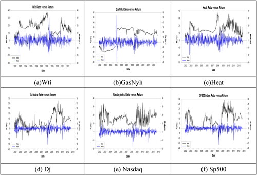
The data in this study included the Wti, GasNyh, Heat, Dj, Sp500, Nasdaq, and UDI.¹² Moreover, the daily close price data of seven assets covered the period from October 23, 2003 to August 5, 2015.¹³ Notably, the study period was divided into the pre-SB and post-SB periods according to the dates of SB obtained by the following procedure. The present study used the univariate GJR-GARCH-M-t model to find the dates of SB for three oil-related assets and the three stock indices via utilizing the maximum likelihood-ratio test of Eizaguirre et al. (2004). Then, for each of six assets, I got a series of likelihood-ratio statistics (LRS) of the alternative hypothesis of one single SB point against the null hypothesis of no SB point. Figure 1 depicted the trends of the series of both return and the above LRS for the six assets, and I found that the maximum values of LRS (i.e., Max. LRS) for the Wti, GasNyh, Heat, Sp500, Nasdaq, and Dj respectively were 38.978 (May 21, 2008), 30.605 (June 11, 2008), 37.807 (July 2, 2008), 29.276 (November 4, 2009), 35.099 (August 4, 2010), and 28.061 (November 10, 2010).¹⁴ The above Max. LRS were all greater than 25.22, indicating that the date occurring the Max. LRS was the date of SB.¹⁵ Hence, for the above six assets, the dates of SB covered the period from May 21, 2008 for the Wti to November 10, 2010 for the Dj. The above SB period seems to overlap with the period of both the GFC happening and QE policy implemented.¹⁶ Moreover, the assets in the oil market occured the SB earlier than the assets in the stock market.

Figure 1. The trend of return and likelihood ration (a) Wti (b) GasNyh (c) Heat (d) Dj (e) Nasdaq (f) Sp500.

Source: Author.

Table 1 reports the basic statistical characteristics of daily return for the seven assets in the US during the overall period and two subperiods.¹⁷ The descriptive statistics at panel A represents the average status of that descriptive statistics for the overall period. Conversely, the descriptive statistics at panel B and panel C can describe the status of that descriptive statistics during the pre-SB and post-SB periods, respectively. Subsequently, I mainly analyse the variation of the values of the mean and standard deviation for the overall period and the two subperiods to inspect whether the return series of six assets actually exists the SB.¹⁸ Regarding each of three oil-related assets, the values of mean return for the pre-SB and post-SB periods were respectively greater and smaller than those for the overall period. As to each of three stock indices, the values of mean return for the pre-SB and post-SB periods were respectively smaller and greater than those for the overall period. Conversely, except for the Wti, the values of standard deviation for the pre-SB and post-SB periods were respectively greater and smaller than those for the overall period. From the above phenomenon, I find that, for most of the assets in the oil and stock markets, the values of mean return or standard deviation for the pre-SB and post-SB periods were significantly different, indicating that the SB really happened at the return series of assets in the oil and stock markets. For example, the values of mean return during the pre-SB period were significantly greater and smaller than the values of mean return during the post-SB period for the oil assets and stock indices, respectively.

Table 1. Descriptive statistics of daily return for the overall, pre-SB and post-SB periods.

	Mean	SD	Max.	Min.	SK	KUR	J-B	$Q^2(24)$	Obs.
Panel A. The overall period
Wti	0.0136	2.3569	16.413	−12.826	−0.0533	4.8501^c	2880.09^c	3156.1^c	2937
GasNyh	0.0218	2.6364	23.505	−17.889	0.1445^c	6.5263^c	5222.61^c	1374.7^c	2937
Heat	0.0183	2.1441	12.212	−11.421	−0.0224	2.3382^c	669.350^c	871.5^c	2937
Dj	0.0200	1.1262	10.325	−8.200	−0.1947^c	11.194^c	15355.0^c	6232.1^c	2937
Nasdaq	0.0331	1.3247	9.106	−9.587	−0.4168^c	6.5337^c	5309.27^c	5497.8^c	2937
Sp500	0.0237	1.2257	10.423	−9.469	−0.4269^c	11.719^c	16896.7^c	6204.3^c	2937
UDI	0.0015	0.4875	2.155	−4.107	−0.2865^c	3.7235^c	1736.84^c	809.6^c	2937
Panel B. The pre-SB period
Wti	0.1302	2.0667	8.408	−12.390	−0.2366^c	1.487^c	115.5^c	56.0^c	1138
GasNyh	0.1167	2.9131	23.505	−17.889	0.3348^c	7.306^c	2583.7^c	587.5^c	1152
Heat	0.1373	2.3060	11.022	−9.042	0.1959^c	0.601^c	25.0^c	136.2^c	1167
Dj	0.0086	1.2657	10.325	−8.200	−0.1094^a	10.738^c	8445.3^c	3857.8^c	1757
Nasdaq	0.0101	1.4869	9.106	−9.587	−0.3693^c	6.075^c	2636.4^c	3388.2^c	1689
Sp500	0.0000	1.4176	10.423	−9.469	−0.3670^c	11.407^c	8182.5^c	3378.0^c	1503
UDI	–	–	–	–	–	–	–	–	–
Panel C. The post-SB period
Wti	-0.060	2.5211	16.413	−12.826	0.040	5.5312^c	2293.7^c	2337.4^c	1799
GasNyh	-0.039	2.4402	17.367	−15.690	−0.099^a	4.8234^c	1733.3^c	1189.7^c	1785
Heat	-0.060	2.0271	12.212	−11.421	−0.268^c	4.0149^c	1210.0^c	729.6^c	1770
Dj	0.0368	0.8784	4.153	−5.706	−0.472^c	4.4146^c	1002.1^c	980.9^c	1180
Nasdaq	0.0643	1.0663	5.159	−7.148	−0.444^c	4.0049^c	875.1^c	893.8^c	1248
Sp500	0.0485	0.9850	4.631	−6.895	−0.458^c	4.5617^c	1293.6^c	1025.2^c	1434
UDI	–	–	–	–	–	–	–	–	–

Notes: 1. The superscripts a, b and c at a specific descriptive statistics denote the descriptive statistics is significant at the 10%, 5% and 1% levels, respectively. 2. SK and KUR denote the skewness and excess kurtosis, respectively. 3. J-B statistics are based on Jarque and Bera (1987) and are asymptotically chi-squared-distributed with 2 degrees of freedom. 4. $Q^2(24)$ statistics are asymptotically chi-squared-distributed with 24 degrees of freedom. 5. Obs. denotes the number of observation. 6. The dates of structural breaks for the Wti, GasNyh, Heat, Sp500, Nasdaq, and Dj are 2008/5/21, 2008/6/11, 2008/7/2, 2009/11/4, 2010/8/4, and 2010/11/10, respectively. 7. The overall period is from Oct. 22, 2003 to Aug. 5, 2015. 8. The bold (resp. italic) font in column Mean or SD denotes the larger (resp. smaller) value of mean or standard deviation, when the values of Mean or SD for the overall period are compared with those for the pre-SB or post-SB period.

Source: Author.

4. Empirical results

In this section, the results of B-GJR-GARCH-SB model listed in Tables 2 and 3 are used to perform the status variation analysis of each financial feature for two subperiods and further explore the following two questions.¹⁹ First, whether the status of three pairwise markets’ interaction indicators (respectively, two single market indicators) in the three types of paired market (respectively, the three markets) was different before and after the SB. Second, how the SB affected the status of three pairwise markets’ interaction indicators for three types of paired market and the status of two single market indicators in each of three markets. Table 2 (respectively, Table 3) lists the empirical results of the B-GJR-GARCH-SB model for nine oil-stock paired market data (respectively, three oil-FX paired market data and three stock-FX paired market data).²⁰ However, it isn’t easy to give the conclusions for the above analysis. Hence, via the results of B-GJR-GARCH-SB model, I summarize the findings into five tables at the following subsections to perform the status variation analysis of five financial features during pre- and post-SB periods.

Table 2. Empirical results of B-GJR-GARCH-SB model for the Oil-stock paired market data.

	Wti- Dj	Wti- Nasdaq	Wti- Sp500	GasNyh- Dj	GasNyh- Nasdaq	GasNyh- Sp500	Heat- Dj	Heat- Nasdaq	Heat- Sp500
Panel A. Return spillover
${\varphi }_{12}^B$	0.1134 (0.061)^a	0.1182 (0.048)^b	0.1486 (0.058)^b	0.1716 (0.079)^b	0.1777 (0.062)^c	0.1872 (0.074)^b	0.1031 (0.063)	0.1357 (0.050)^c	0.1193 (0.060)^b
${\varphi }_{12}^A$	−0.0314 (0.052)	−0.0137 (0.040)	0.0021 (0.041)	−0.0046 (0.057)	0.0150 (0.044)	−0.0101 (0.045)	−0.0012 (0.041)	0.0028 (0.032)	0.0112 (0.034)
${\varphi }_{21}^B$	−0.0064 (0.009)	−0.0116 (0.012)	−0.0044 (0.009)	−0.0050 (0.006)	−0.0037 (0.008)	−0.0010 (0.006)	−0.0092 (0.008)	−0.0186 (0.010)^a	−0.0062 (0.008)
${\varphi }_{21}^A$	0.0128 (0.010)	0.0173 (0.013)	0.0126 (0.010)	0.0127 (0.010)	0.0209 (0.012)^a	0.0163 (0.009)^a	0.0009 (0.012)	0.0026 (0.015)	0.0019 (0.011)
Panel B. Risk premium
${\tau }_1^B$	0.1343 (0.048)^c	0.1382 (0.040)^c	0.1465 (0.053)^c	−0.0099 (0.053)	0.0082 (0.055)	−0.0254 (0.072)	0.0871 (0.048)^a	0.0928 (0.043)^b	0.0913 (0.046)^b
${\tau }_1^A$	0.0826 (0.064)	0.0764 (0.048)	0.0979 (0.065)	−0.1300 (0.078)^a	−0.1122 (0.081)	−0.1347 (0.109)	0.0619 (0.082)	0.0620 (0.068)	0.0881 (0.067)
${\tau }_2^B$	0.0410 (0.022)^a	0.0852 (0.057)	0.0927 (0.026)^c	0.0300 (0.025)	0.0695 (0.055)	0.0832 (0.028)^c	0.0274 (0.019)	0.0633 (0.054)	0.0723 (0.022)^c
${\tau }_2^A$	0.0127 (0.018)	0.0693 (0.039)^a	0.0558 (0.023)^b	0.0304 (0.025)	0.0698 (0.046)	0.0569 (0.029)^a	0.0308 (0.020)	0.0674 (0.045)	0.0629 (0.025)^b
Panel C. Volatility spillover
${\theta }_{12}^B$	0.0649 (0.022)^c	0.0385 (0.015)^b	0.0488 (0.019)^b	0.1225 (0.056)^b	0.0861 (0.039)^b	0.1039 (0.057)^a	0.0200 (0.015)	0.0161 (0.008)^a	0.0155 (0.012)
${\theta }_{12}^A$	−0.0047 (0.012)	−0.0060 (0.008)	−0.0011 (0.009)	−0.0095 (0.015)	−0.0064 (0.011)	0.0011 (0.012)	−0.0046 (0.004)	−0.0035 (0.003)	−0.0017 (0.003)
${\theta }_{21}^B$	0.0016 (0.000)^b	0.0013 (0.001)	0.0002 (0.000)	0.0002 (0.000)	−0.0001 (0.000)	−0.0000 (0.000)	0.0001 (0.000)	0.0000 (0.000)	−0.0003 (0.000)
${\theta }_{21}^A$	0.0014 (0.000)	0.0003 (0.001)	0.0003 (0.000)	0.0004 (0.000)	−0.0012 (0.001)	0.0000 (0.000)	0.0006 (0.001)	0.0000 (0.001)	0.0003 (0.001)
Panel D. Correlation
${\omega }_{12}^B$	−0.0052 (0.003)^a	−0.0046 (0.003)	−0.0013 (0.002)	−0.0058 (0.003)	−0.0053 (0.004)	−0.0013 (0.003)	−0.0056 (0.003)^a	−0.0048 (0.003)	−0.0015 (0.003)
${\omega }_{12}^A$	0.0084 (0.002)^c	0.0113 (0.003)^c	0.0110 (0.003)^c	0.0093 (0.003)^b	0.0089 (0.003)^c	0.0098 (0.003)^c	0.0057 (0.002)^c	0.0068 (0.002)^b	0.0075 (0.002)^c
Panel E. Leverage effect
${\mathrm{\zeta }}_1^B$	0.0474 (0.009)^c	0.0411 (0.010)^c	0.0511 (0.010)^c	0.0097 (0.014)	−0.0003 (0.014)	0.0160 (0.015)	0.0210 (0.010)^b	0.0183 (0.009)^a	0.0213 (0.009)^b
${\mathrm{\zeta }}_1^A$	0.0436 (0.008)^c	0.0430 (0.009)^c	0.0421 (0.008)^c	−0.0016 (0.013)	−0.0079 (0.012)	−0.0158 (0.011)	0.0036 (0.008)	0.0072 (0.007)	0.0010 (0.007)
${\mathrm{\zeta }}_2^B$	0.1758 (0.017)^c	0.1386 (0.018)^c	0.1535 (0.014)^c	0.1841 (0.018)^c	0.1437 (0.020)^c	0.1714 (0.018)^c	0.1648 (0.017)^c	0.1314 (0.019)^c	0.1488 (0.014)^c
${\mathrm{\zeta }}_2^A$	0.1756 (0.019)^c	0.1346 (0.018)^c	0.1554 (0.015)^c	0.1862 (0.020)^c	0.1366 (0.019)^c	0.1766 (0.019)^c	0.1606 (0.019)^c	0.1186 (0.018)^c	0.1443 (0.015)^c
Panel F. The others information
$\mathrm{\nu }$	8.8100 (0.687)^c	9.4889 (0.778)^c	8.3085 (0.648)^c	8.9611 (0.781)^c	9.2629 (0.847)^c	8.4186 (0.674)^c	10.1589 (0.954)^c	10.4301 (1.016)^c	9.4691 (0.841)^c
$Q_1^2(24)$	25.555	25.988	25.512	74.986^c	72.908^c	65.101^c	78.295^c	82.578^c	79.687^c
$Q_2^2(24)$	31.170	32.881	32.638	30.759	33.022	31.068	31.535	31.715	30.497
Panel G. The settings for the pre- and post-SB periods
Pre-SB	2003/10/22- 2008/5/21	2003/10/22- 2008/5/21	2003/10/22- 2008/5/21	2003/10/22- 2008/6/11	2003/10/22- 2008/6/11	2003/10/22- 2008/6/11	2003/10/22- 2008/7/02	2003/10/22- 2008/7/02	2003/10/22- 2008/7/02
Post-SB	2010/11/10- 2015/08/05	2010/08/04- 2015/08/05	2009/11/04- 2015/08/05	2010/11/10- 2015/08/05	2010/08/04- 2015/08/05	2009/11/04- 2015/08/05	2010/11/10- 2015/08/05	2010/08/04- 2015/08/05	2009/11/04- 2015/08/05

Note: 1. The superscripts a, b and c at a specific parameter denote the parameter is significant at the 10%, 5% and 1% levels, respectively. 2. Numbers in parentheses at the row of parameters are the standard errors. 3. $Q_i^2\left(24\right)$ for $\mathrm{i}=1,2\mathrm{ }$ statistics are asymptotically chi-squared-distributed with 24 degrees of freedom. 4. The date period at the row ‘Pre-SB’ (respectively, ‘Post-SB’) denotes the starting date and ending date for the pre-SB (respectively, post-SB) period.

Source: Author.

Table 3. Empirical results of B-GJR-GARCH-SB model for the Oil-FX and Stock-FX types of paired market data.

	Wti- UDI	GasNyh- UDI	Heat- UDI	Dj- UDI	Nasdaq- UDI	Sp500- UDI
Panel A. Return spillover
${\varphi }_{12}^B$	−0.0508 (0.122)	0.1036 (0.155)	0.0486 (0.135)	−0.0555 (0.038)	−0.0570 (0.052)	−0.0518 (0.045)
${\varphi }_{12}^A$	−0.0086 (0.088)	0.0576 (0.100)	−0.1426 (0.079)^a	0.0024 (0.044)	−0.0173 (0.057)	−0.0047 (0.041)
${\varphi }_{21}^B$	−0.0207 (0.005)^c	−0.0125 (0.004)^c	−0.0165 (0.005)^c	−0.0731 (0.009)^c	−0.0627 (0.008)^c	−0.0823 (0.009)^c
${\varphi }_{21}^A$	−0.0096 (0.004)^b	−0.0056 (0.004)	−0.0073 (0.005)	−0.0249 (0.011)^b	−0.0188 (0.010)^a	−0.0233 (0.010)^b
Panel B. Risk premium
${\tau }_1^B$	0.1156 (0.054)^b	0.0532 (0.055)	0.0896 (0.047)^a	0.0291 (0.022)	0.0473 (0.039)	0.0601 (0.020)^c
${\tau }_1^A$	0.0152 (0.055)	−0.0383 (0.066)	0.0025 (0.054)	0.0222 (0.022)	0.0287 (0.041)	0.0252 (0.022)
${\tau }_2^B$	0.0157 (0.013)	0.0142 (0.011)	0.0144 (0.011)	0.0154 (0.010)	0.0119 (0.013)	0.0086 (0.011)
${\tau }_2^A$	−0.0069 (0.011)	−0.0091 (0.009)	−0.0087 (0.009)	−0.0046 (0.008)	−0.0061 (0.011)	−0.0111 (0.010)
Panel C. Volatility spillover
${\theta }_{12}^B$	0.6403 (0.223)^c	1.8544 (0.531)^c	0.5122 (0.174)^c	0.0436 (0.014)^c	0.1050 (0.050)^b	0.0391 (0.018)^b
${\theta }_{12}^A$	0.2667 (0.151)^a	0.5996 (0.263)^b	0.0959 (0.079)	0.0467 (0.017)^c	0.1285 (0.048)^c	0.0690 (0.016)^c
${\theta }_{21}^B$	0.0002 (0.000)^a	0.0000 (0.000)	0.0002 (0.000)	0.0009 (0.000)^b	0.0009 (0.000)^c	0.0008 (0.000)^c
${\theta }_{21}^A$	0.0006 (0.000)^c	0.0005 (0.000)^c	0.0010 (0.000)^c	0.0001 (0.000)	0.0000 (0.000)	0.0002 (0.000)
Panel D. Correlation
${\omega }_{12}^B$	−0.0006 (0.000)	−0.0003 (0.000)	−0.0006 (0.000)	−0.0002 (0.000)	0.0000 (0.000)	−0.0001 (0.000)
${\omega }_{12}^A$	−0.0002 (0.000)	−0.0003 (0.000)	−0.0001 (0.000)	−0.0000 (0.000)	0.0001 (0.000)	−0.0001 (0.000)
Panel E. Leverage effect
${\mathrm{\zeta }}_1^B$	0.0397 (0.013)^c	0.0014 (0.020)	0.0144 (0.012)	0.1753 (0.012)^c	0.1724 (0.023)^c	0.1717 (0.017)^c
${\mathrm{\zeta }}_1^A$	0.0573 (0.012)^c	0.0175 (0.014)	0.0248 (0.009)^c	0.1568 (0.014)^c	0.1416 (0.022)^c	0.1466 (0.016)^c
${\mathrm{\zeta }}_2^B$	0.0070 (0.009)	0.0036 (0.010)	0.0032 (0.010)	−0.0157 (0.007)^b	−0.0207 (0.007)^c	−0.0119 (0.008)
${\mathrm{\zeta }}_2^A$	−0.0079 (0.007)	−0.0180 (0.007)^b	−0.0204 (0.007)^c	−0.0162 (0.007)^b	−0.0123 (0.007)^a	−0.0092 (0.006)
Panel F. The others information
$\mathrm{\nu }$	10.1214 (0.893)^c	11.0052 (1.084)^c	11.1321 (1.117)^c	9.9458 (1.001)^c	11.3468 (1.332)^c	9.7158 (0.938)^c
$Q_1^2(24)$	27.223	50.022^c	63.008^c	26.707	29.900	24.782
$Q_2^2(24)$	39.895^b	34.632^a	36.185^a	38.410^b	39.963^b	38.722^b
Panel G. The settings for the pre- and post-SB periods
Pre-SB	2003/10/22- 2008/5/21	2003/10/22- 2008/6/11	2003/10/22- 2008/7/02	2003/10/22- 2010/11/10	2003/10/22- 2010/8/04	2003/10/22- 2009/11/04
Post-SB	2008/05/21- 2015/08/05	2008/06/11- 2015/08/05	2008/07/02- 2015/08/05	2010/11/10- 2015/08/05	2010/08/04- 2015/08/05	2009/11/04- 2015/08/05

Note: 1. Please see the notes 1–4 in Table 2.

Source: Author.

4.1. How did the structural break affect the return and volatility spillovers between two markets?

This subsection considers whether the status of the return (or volatility) spillover was different before and after the date of the SB and how the SB affected the status of the return (or volatility) spillover. Subsequently, I condensed the results of parameters ${\mathrm{\varphi }}_{12}^{\mathrm{B}},$ ${\mathrm{\varphi }}_{12}^{\mathrm{A}},$ ${\mathrm{\varphi }}_{21}^{\mathrm{B}}$ and ${\mathrm{\varphi }}_{21}^{\mathrm{A}}$ in Tables 2 and 3 into Table 4 regarding the return spillover. Moreover, I condensed the results of parameters ${\mathrm{\theta }}_{12}^{\mathrm{B}},$ ${\mathrm{\theta }}_{12}^{\mathrm{A}},$ ${\mathrm{\theta }}_{21}^{\mathrm{B}},$ and ${\mathrm{\theta }}_{21}^{\mathrm{A}}$ in Tables 2 and 3 into Table 5 regarding the volatility spillover. Then, I take the example of return spillover to illustrate the above process. First, I employ panel A and panel B of Table 4 to summarize the results from the values of parameters ${\mathrm{\varphi }}_{12}^{\mathrm{B}},$ ${\mathrm{\varphi }}_{12}^{\mathrm{A}},$ ${\mathrm{\varphi }}_{21}^{\mathrm{B}}$ and ${\mathrm{\varphi }}_{21}^{\mathrm{A}}$ respectively in panel A of Tables 2 and 3. The significance on parameters ‘${\mathrm{\varphi }}_{12}^{\mathrm{B}}$ and ${\mathrm{\varphi }}_{21}^{\mathrm{B}}$’ and ‘${\mathrm{\varphi }}_{12}^{\mathrm{A}},$ and ${\mathrm{\varphi }}_{21}^{\mathrm{A}}$’ can determine the status of the spillover on the return respectively for the pre-SB and post-SB periods.²¹ Taking the example of Heat-Nasdaq pair of data in Table 2, the value of parameter ${\mathrm{\varphi }}_{12}^{\mathrm{B}}\mathrm{ }$(0.1357) is significantly positive. During the pre-SB period, a positive return spillover from the second asset (Nasdaq) to the first asset (Heat) exists. Conversely, the value of parameter ${\mathrm{\varphi }}_{21}^{\mathrm{B}}$ (-0.0186) is significantly negative. During the pre-SB period, a negative return spillover from the first asset (Heat) to the second asset (Nasdaq) exists. Then, the symbols ‘←(+) and →(−)’ representing the bidirectional return spillovers are recorded in the row ‘Pre-SB’ and column ‘Heat-Nasdaq’ of the panel A in Table 4. Taking another example of ‘Wti-UDI’ pair of data in Table 3, the value of parameter ${\mathrm{\varphi }}_{21}^{\mathrm{B}}$ (−0.0207) is significantly negative. Thus, this result is recorded as ‘→(−)’ in the row ‘Pre-SB’ and column ‘Wti-UDI’ of the panel B in Table 4. However, the value of parameter ${\mathrm{\varphi }}_{21}^{\mathrm{A}}$(−0.0096) is still significantly negative, but it is lower than the value of parameter ${\mathrm{\varphi }}_{21}^{\mathrm{B}}$ (−0.0207) in absolute value. Then, this result is recorded as ‘→(−,↓)’²² in the row ‘Post-SB’ and column ‘Wti-UDI’ in the panel B of Table 4.

Table 4. The summary results of return spillover for 15 pairs of data.

Panel A. The Oil-stock paired market data
	Wti- Dj	Wti- Nasdaq	Wti- Sp500	GasNyh- Dj	GasNyh- Nasdaq	GasNyh- Sp500
Pre-SB	←(+)	←(+)	←(+)	←(+)	←(+)	←(+)
Post-SB	×	×	×	×	→(+)	→(+)
	Heat- Dj	Heat- Nasdaq	Heat- Sp500
Pre-SB	×	←(+) →(-)	←(+)
Post-SB	×	×	×
Panel B. The Oil-FX and Stock-FX types of paired market data
	Wti- UDI	GasNyh- UDI	Heat- UDI	Dj- UDI	Nasdaq- UDI	Sp500- UDI
Pre-SB	→(-)	→(-)	→(-)	→(-)	→(-)	→(-)
Post-SB	→(-,↓)	×	←(-)	→(-,↓)	→(-,↓)	→(-,↓)
Panel C. The summary of return spillover for three types of paired market data
	Oil-stock		Oil-FX		Stock-FX
Pre-SB	Oil$\stackrel{\leftharpoonup }{(+)}\mathrm{Stock}$ $$		$\mathrm{Oil}\stackrel{\rightharpoonup }{(-)}\mathrm{F}\mathrm{X}$		$\mathrm{Stock}\stackrel{\rightharpoonup }{(-)}\mathrm{F}\mathrm{X}$
Post-SB	×		?		$\mathrm{Stock}\stackrel{\rightharpoonup }{(¯,\downarrow )}\mathrm{F}\mathrm{X}$
Panel D. The messages of significant situations for three types of paired market data
	Total	Oil-stock		Oil-FX		Stock-FX
	(o,×)[ o%,S]	(o,×) [o%,S]		(o,×) [o%,S]		(o,×) [o%,S]
Pre-SB	(14,1)[93.3%,⊕]	(8,1)[88.9%,⊕]		(3,0) [100%,⊕]		(3,0) [100%,⊕]
Post-SB	(7,8) [46.7%,⦶]	(2,7) [22.2%,⊗]		(2,1) [66.7%,⦶]		(3,0) [100%,⊕]
difference	−46.6%	−66.7%		−33.3%		0%

Note: 1. The symbol × represents that the return spillover does not exist. 2. The symbol → denotes that the return spillover from the first asset to the second asset significantly exists because the value of parameter ${\varphi }_{21}^B$ or ${\varphi }_{21}^A$ in Tables 2 and 3 is significant. 3. The symbol ← denotes that the return spillover from the second asset to the first asset significantly exists because the value of parameter ${\varphi }_{12}^B$ or ${\varphi }_{12}^A$ in Tables 2 and 3 is significant. 4. The symbol + (respectively, -) inside the bracket beside the symbol → or ← denotes that the return spillover is significantly positive (respectively, negative). 5. The symbol ↑ (respectively, ↓) inside the bracket beside the symbol → or ← corresponding to row ‘Post-SB’ denotes that, based on having the same direction of return spillover for the pre- and post-SB periods, the return spillover exhibits greater (respectively, smaller) after the structural break. 6. The numbers in columns ‘o’ and ‘×’ underneath a specific paired market data (or ‘Total’) at panel D respectively represent the total numbers of significant and insignificant cases for this specific paired market data (or the entire US market). 7. The numbers or symbols in columns ‘o%’ and ‘S’ underneath a specific paired market data (or ‘Total’) at panel D respectively represent the significant ratio and the significant degree for this specific paired market data (or the entire US market). Moreover, the significant ratio equals to the total numbers of significant cases divided by the sum value of the total numbers of significant and insignificant cases. 8. There are three types of significant degree: ‘⊕’, ‘⦶’, and ‘⊗’. The significant degree is determined by its corresponding value of significant ratio. For example, the symbols ‘⊕’ and ‘⊗’ denote the values of significant ratio are greater than 2/3 and smaller than 1/3, respectively. On the other hand, the symbol ‘⦶’denotes the value of significant ratio is between 1/3 and 2/3. Hence, the symbols ‘⊕’ and ‘⦶’ denote the discussed financial feature significantly and slightly exist, respectively. Conversely, the symbol ‘⊗’ denotes the discussed financial feature does not exist. 9. The number at the row ‘difference’ and the column corresponding to 'a specific paired market data' (or ‘Total’) at panel D denotes the difference of two significant ratios corresponding to the pre- and post-SB periods for this specific paired market data (or the entire US market).

Source: Author.

Table 5. The summary results of volatility spillover effect for 15 pairs of data.

Panel A. The Oil-stock paired market data
	Wti- Dj	Wti- Nasdaq	Wti- Sp500	GasNyh- Dj	GasNyh- Nasdaq	GasNyh- Sp500
Pre-SB	←(+) →(+)	←(+)	←(+)	←(+)	←(+)	←(+)
Post-SB	×	×	×	×	×	×
	Heat- Dj	Heat- Nasdaq	Heat- Sp500
Pre-SB	×	←(+)	×
Post-SB	×	×	×
Panel B. The Oil-FX and Stock-FX types of paired market data
	Wti- UDI	GasNyh- UDI	Heat- UDI	Dj- UDI	Nasdaq- UDI	Sp500- UDI
Pre-SB	←(+) →(0,+)	←(+)	←(+)	←(+) →(0,+)	←(+) →(0,+)	←(+) →(0,+)
Post-SB	←(+,↓) →(0,+,↑)	←(+,↓) →(0,+)	→(+)	←(+,↑)	←(+,↑)	←(+,↑)
Panel C. The summary of volatility spillover for three types of paired market data
	Oil-stock		Oil-FX		Stock-FX
Pre-SB	Oil$\stackrel{\leftharpoonup }{(+)}\mathrm{Stock}$		Oil$\stackrel{\leftharpoonup }{(+)}\mathrm{F}\mathrm{X}$		Stock$\stackrel{\leftharpoonup }{(+)}\mathrm{F}\mathrm{X}$
Post-SB	×		$\mathrm{Oil}\stackrel{\leftharpoonup }{(+,\downarrow )}\mathrm{F}\mathrm{X}$		$\mathrm{Stock}\stackrel{\leftharpoonup }{(+,\uparrow )}\mathrm{F}\mathrm{X}$
Panel D. The messages of significant situations for three types of paired market data
	Total	Oil-stock		Oil-FX		Stock-FX
	(o,×)[ o%,S]	(o,×) [ o%,S]		(o,×) [ o%,S]		(o,×) [ o%,S]
Pre-SB	(13,2) [86.7%,⊕]	(7,2) [77.8%,⊕]		(3,0) [100%,⊕]		(3,0) [100%,⊕]
Post-SB	(6,9) [40%,⦶]	(0,9) [0%,⊗]		(3,0) [100%,⊕]		(3,0) [100%,⊕]
difference	−46.7%	−77.8%		0%		0%

Note: 1. The symbol × represents that the volatility spillover does not exist. 2. The symbol → denotes that the volatility spillover from the first asset to the second asset significantly exists because the value of parameter ${\theta }_{21}^B$ or ${\theta }_{21}^A$ in Tables 2 and 3 is significant. 3. The symbol ← denotes the volatility spillover from the second asset to the first asset significantly exists because the value of parameter ${\theta }_{12}^B\mathrm{ }{\text{or θ}}_{12}^{\mathrm{A}}$ in Tables 2 and 3 is significant. 4. The symbol + (respectively, −) inside the bracket beside the symbol → or ← denotes that the volatility spillover is significantly positive (respectively, negative). 5. The symbol ↑(respectively, ↓) inside the bracket beside the symbol → or ← corresponding to row ‘Post-SB’ denotes that, based on having the same direction of volatility spillover for the pre- and post-SB periods, the volatility spillover exhibits greater (respectively, smaller) after the structural break. 6. The number '0' inside the bracket beside the symbol → or ← denotes that the volatility spillover is very small because the value of the corresponding parameter is smaller than 0.001. 7. As to the others notes, please see the notes 6–9 in Table 4.

Source: Author.

Panels A and B of Table 4 report the results of return spillover for 15 pairs of data during the two subperiods. Then, I condense the results of panels A and B into panels C and D to depict the status variation of the return spillover during two subperiods for three types of paired markets. First, in panel A of Table 4, I find that there exists a positive return spillover from the stock market to the oil market during the pre-SB period because the symbol ‘←(+)’ appears for most of oil-stock paired market data (7/9).²³ Then, I mark the ‘Oil$\stackrel{\leftharpoonup }{(+)}\mathrm{Stock}$’ in the row ‘Pre-SB’ and column ‘Oil-Stock’ of panel C in Table 4. Conversely, there does not exist the return spillover between the oil market and stock market during the post-SB period because the symbol ‘×’ appears for most of oil-stock paired market data (7/9). Then, I mark the ‘×’ in the row ‘Post-SB’ and column ‘Oil-Stock’ of panel C in Table 4. Second, in panel B of Table 4, I find that there exists two negative return spillovers respectively from the oil market and stock market to the FX market during the pre-SB period because the symbol ‘→(−)’ appears for both oil-FX and oil-stock paired market data (3/3). Then, in panel C of Table 4, I mark the ‘$\mathrm{Oil}\stackrel{\leftharpoonup }{(-)}\mathrm{F}\mathrm{X}$’ and ‘$\mathrm{Stock}\stackrel{\leftharpoonup }{(-)}\mathrm{F}\mathrm{X}$’ in the row ‘Pre-SB’ and columns ‘Oil-FX’ and ‘Stock-FX’, respectively. Moreover, I find that it is uncertain for the return spillover between the oil market and FX market during the post-SB period because there isn’t a consistent result for three oil-FX paired market data. That is, three different symbols ‘→(−,↓)’, ‘×’ and ‘←(-)’ appear at the Wti-UDI, GasNyh-UDI and Heat-UDI pairs of data, respectively. Then, I mark the ‘?’ in the row ‘Post-SB’ and column ‘Oil-FX’ of panel C in Table 4. Additionally, I find that, in panel B of Table 4, the symbol ‘→(−,↓)’ appears at the row ‘Post-SB’ for all three Stock-FX paired market data. Then, I mark the ‘$\mathrm{Stock}\stackrel{\rightharpoonup }{(¯,\downarrow )}\mathrm{F}\mathrm{X}$’ in the row ‘Post-SB’ and column ‘Stock-FX’ of panel C in Table 4. Finally, regarding the results of panels A and B in Table 4, I calculate the messages of significant situations for three types of paired market data and even for the entire three markets of US, and record them in panel D of Table 4. The messages of significant situation include the significant ratio, the degree of significance and the total numbers of significant and insignificant cases for two subperiods, and the difference of significant ratios between two subperiods. Taking the example of oil-stock paired market data during the pre-SB period, only Heat-Dj pair of data isn’t significant. The total numbers of significant and insignificant cases for the oil-stock paired market data are 8 and 1, respectively. Its corresponding significant ratio is 88.9% (= 8/9). This is greater than 2/3, so the degree of significance is record as ‘⊕’.²⁴ Then, in the row ‘Pre-SB’ in panel D, I record ‘(8, 1)’ and ‘[88.9%,⊕]’, respectively in the columns ‘(o,×)’ and ‘[o%,S]’, which are under ‘Oil-stock’. At the same inference process, during the post-SB period, the total numbers of significant and insignificant cases for the oil-stock paired market data are 2 and 7, respectively. Its significant ratio is 22.2% (=2/9). Hence, the difference of the significant ratios between two subperiods is −66.7% (=22.2% − 88.9%). Then, this number is recorded in the row ‘difference’ and column ‘Oil-stock’ in panel D. To sum up, panels C and D of Table 4 report the summary status of return spillover and its corresponding messages of significant situations for three types of paired market during the two subperiods.

The following can be concluded from the results listed in panels C and D of Table 4. First, during the pre-SB and post-SB periods, the status of return spillover was significantly different for the oil-stock and oil-FX paired markets, and the entire US market because its corresponding values of the difference of significant ratios were −66.7%, −33.3%, and −46.6%, respectively. Conversely, the status of return spillover was the same for the stock-FX paired market because the difference in significant ratios was 0%. Therefore, Hypothesis 1 was rejected only for the stock-FX paired market (0%). In particular, after the SB, the impact of the return spillover significantly decreased in the US market (−46.6%), especially for the oil-stock paired market (−66.7%). Second, during the pre-SB period, the stock market had a positive impact on the oil market as shown by the symbol ‘Oil$\stackrel{\leftharpoonup }{(+)}\mathrm{Stock}$’. This result is contradictory with the findings from Cevik et al. (2020) which stated that the oil market had an impact on the stock market.²⁵ Moreover, the oil market had a negative impact on the FX market as shown by the symbol ‘$\mathrm{Oil}\stackrel{\leftharpoonup }{(-)}\mathrm{F}\mathrm{X}$’. This result is line with the finding of Amano and Norden (1998).²⁶ Therefore, the stock market affected the FX market. The symbol ‘$\mathrm{Stock}\stackrel{\leftharpoonup }{(-)}\mathrm{F}\mathrm{X}$’ confirmed the above inference and further indicated that the stock market had a negative impact on the FX market. This result is consistent with the findings of Yang and Doong (2004), Kumar (2013) and Erdoğan et al. (2020).²⁷ Hence, among three markets, the stock market possessed the most influential role, followed by the oil market, whereas the FX market had the least influential role. Because the stock market affected both the oil and FX markets whereas the FX market was affected by both the stock and oil markets. However, after the SB, only the phenomenon of ‘the stock market had a negative impact on the FX market’ still existed but its intensity became lower. Thus, during two subperiods, the stock market dominated on the return spillover within three markets of US. To sum up, the status of the return spillover in the US market was significantly different before and after the SB, especially for the oil-stock paired market. Moreover, after the SB, the impact of the return spillover significantly decreased in the US market attributing to the significantly weakening of the phenomenon of ′the stock market having a positive impact on the oil market′ at the pre-SB period.²⁸ Additionally, regarding the return spillover, the stock market dominated within three markets of US during the two subperiods.

Subsequently, I use the summary results of the volatility spillover listed in Table 5 to discuss whether the status of volatility spillover was different before and after the date of SB and how the SB affected the status of the volatility spillover.²⁹ Based on the results listed in panels C and D of Table 5, I got the following conclusions. First, during the pre-SB and post-SB periods, the status of volatility spillover was significantly different for the oil-stock paired market and the entire US market because its corresponding values of difference of significant ratios were −77.8% and −46.7%, respectively. Conversely, the status of volatility spillover was the same for both the oil-FX and Stock-FX paired markets related with the FX market because the values of difference in significant ratios were all 0%. Hence, Hypothesis 2 was rejected for both the oil-FX and stock-FX paired markets (0%). In particular, after the SB, the impact of the volatility spillover significantly decreased in the US market (−46.7%), especially for the oil-stock paired market (−77.8%). Second, during the pre-SB period, the FX market had a positive impact on the stock market as shown by the symbol ‘$\mathrm{Stock}\stackrel{\leftharpoonup }{\left(+\right)}\mathrm{F}\mathrm{X}$’. This result is partially consistent with the finding of Su (2015).³⁰ Moreover, the stock market had a positive impact on the oil market as shown by the symbol ‘Oil$\stackrel{\leftharpoonup }{(+)}\mathrm{Stock}$’. This result is consistent with the findings of Jebabli, et al. (2021) and Gomez-Gonzalez, et al. (2021).³¹ Therefore, the FX market affected the oil market. The symbol ‘Oil$\stackrel{\leftharpoonup }{\left(+\right)}\mathrm{F}\mathrm{X}$’ confirmed the above inference and further indicated that the FX market has a positive impact on the oil market. This result is in line with the finding of Hameed, et al. (2021).³² Hence, among three markets, the FX market possessed the most influential role, followed by the stock market, whereas the oil market had the least influential role. The reason was that the FX market affected both the oil and stock markets whereas the oil market was affected by both the stock and FX markets. However, after the SB, the phenomena of ‘the FX market had a positive impact on the oil and stock markets’ still existed but its intensity became lower and higher, respectively. Thus, during two subperiods, the FX market dominated on the volatility spillover within three markets of US. To sum up, the status of the volatility spillover in the US market was significantly different before and after the SB, especially for the oil-stock paired market. Moreover, after the SB, the impact of the volatility spillover significantly decreased in the US market attributing to the completely disappearing of the phenomenon of ′the stock market having a positive impact on the oil market′ at the pre-SB period.³³ Additionally, regarding the volatility spillover, the FX market dominated within three markets of US during the two subperiods.

4.2. How did the structural break affect the correlation between two markets?

This subsection considers whether the status of the correlation was different before and after the date of the SB and how the SB affected the status of the correlation. The present study uses the conditional covariance to measure the correlation as illustrated in section 2. Then, I employ panel A and panel B of Table 6 to summarize the results from the values of parameters ${\omega }_{12}^B$ and ${\omega }_{12}^A$ respectively in panel D of Tables 2 and 3. The significance on parameters ${\omega }_{12}^B$ and ${\omega }_{12}^A$ can determine the states of the correlation respectively for the pre-SB and post-SB periods.³⁴ Taking the example of Wti-Dj pair of data in Table 2, the values of parameters ${\omega }_{12}^B$(-0.0052) and ${\omega }_{12}^A$(0.0084) are significantly negative and positive, respectively. Thus, the negatively and positively correlations exist between two assets, the Wti and Dj, respectively during the pre-SB and post-SB periods. Then, the symbols ‘-’ and ‘+’ are recorded in the column ‘Wti-Dj’ and the rows ‘Pre-SB’ and ‘Post-SB’ of the panel A in Table 6, respectively.

Table 6. The summary results of correlation for 15 pairs of data.

Panel A. The Oil-stock paired market data
	Wti- Dj	Wti- Nasdaq	Wti- Sp500	GasNyh- Dj	GasNyh- Nasdaq	GasNyh- Sp500
Pre-SB	–	×(-)	×(-)	×(-)	×(-)	×(-)
Post-SB	+	+	+	+	+	+
	Heat- Dj	Heat- Nasdaq	Heat- Sp500
Pre-SB	–	×(-)	×(-)
Post-SB	+	+	+
Panel B. The Oil-FX and Stock-FX types of paired market data
	Wti- UDI	GasNyh- UDI	Heat- UDI	Dj- UDI	Nasdaq- UDI	Sp500- UDI
Pre-SB	×(0,-)	×(0,-)	×(0,-)	×(0,-)	×(0,+)	×(0,-)
Post-SB	×(0,-)	×(0,-)	×(0,-)	×(0,-)	×(0,+)	×(0,-)
Panel C. The summary of correlation for three types of paired market data
	Oil-stock		Oil-FX		Stock-FX
Pre-SB	×(-)		×(0,-)		×(0,-)
Post-SB	+		×(0,-)		×(0,-)
Panel D. The messages of significant situations for three types of paired market data
	Total	Oil-stock		Oil-FX		Stock-FX
	(o,×)[ o%,S]	(o,×) [ o%,S]		(o,×) [ o%,S]		(o,×) [ o%,S]
Pre-SB	(2,13)[13.3%,⊗]	(2,7) [22.2%,⊗]		(0,3) [0%,⊗]		(0,3) [0%,⊗]
Post-SB	(9,6) [60%,⦶]	(9,0) [100%,⊕]		(0,3) [0%,⊗]		(0,3) [0%,⊗]
difference	46.7%	77.8%		0%		0%

Note: 1. In this table, I use the conditional covariance to represent the correlation. 2. The symbol + (respectively, −) denotes that the correlation is significantly positive (respectively, negative) because the value of parameter ${\omega }_{12}^B$ or ${\omega }_{12}^A$ in Tables 2 and 3 is significantly positive (respectively, negative). 3. The symbol × represents that the correlation does not exist. 4. The symbol + (respectively, −) inside the bracket beside the symbol × denotes that the value of correlation is positive (respectively, negative) but isn’t significant. 5. The number ‘0’ inside the bracket beside the symbol × denotes that the value of correlation is smaller than 0.001. 6. As to the others notes, please see the notes 6–9 in Table 4.

Source: Author.

Panels A and B of Table 6 show the results of correlation for 15 pairs of data during the two subperiods. Then, with the same inference process described in Section 4.1, I condense the results of panels A and B into panels C and D to depict the status variation of the correlation during two subperiods for three types of paired markets. For example, in panel A of Table 6, I find that there isn’t any correlation between the oil market and stock market during the pre-SB period because the symbol ‘×(-)’ appears for most of oil-stock paired market data (7/9). Then, I record the ‘×(-)’ in the row ‘Pre-SB’ and column ‘Oil-stock’ of panel C in Table 6. Conversely, I find that there exists a positive correlation between the oil market and stock market during the post-SB period because the symbol ‘+’ appears for all oil-stock paired market data. Then, I record the ‘+’ in the row ‘Post-SB’ and column ‘Oil-Stock’ of panel C in Table 6. As to the messages of significant situation of oil-stock paired market data during the pre-SB period, only Wti-Dj and Heat-Dj pairs of data are significant. Thus, the total numbers of significant and insignificant cases for the oil-stock paired market data are 2 and 7, respectively. Its corresponding significant ratio is 22.2% (= 2/9). This is smaller than 2/3, thus the degree of significance is record as ‘⊗’. Then, in row ‘Pre-SB’ of panel D, I record ‘(2, 7)’ and ‘[22.2%,⊗]’, respectively in the columns ‘(o,×)’ and ‘[o%,S]’, which are under ‘Oil-stock’. Hence, panels C and D of Table 6 report the summary status of correlation and its corresponding messages of significant situations for three types of paired market during the two subperiods.

The following can be concluded from the results listed in panels C and D of Table 6. First, during the pre-SB and post-SB periods, the status of correlation was significantly different for the oil-stock paired market and the entire US market because its corresponding values of the difference of significant ratios were 77.8% and 46.7%, respectively. Conversely, the status of correlation was practically the same for the oil-FX and stock-FX paired markets related with the FX market because its corresponding values of the difference in significant ratios were all 0%. Therefore, Hypothesis 3 was rejected for both the oil-FX market (0%) and stock-FX market (0%). In particular, after the SB, the impact of the correlation significantly increased in the US market (46.7%), especially for the oil-stock paired market (77.8%). Second, during the pre-SB period, the correlation did not exist for three types of paired market, especially for the oil-FX and stock-FX paired markets related with the FX market. These results are partially consistent with Chang, et al. (2013), who found that the correlations across the oil and stock markets were very low, and were less significant. However, after the SB, ‘the correlation did not exist for three types of paired market’ was transferred into ‘only a positive correlation between the oil and stock markets existed’ with the significance ratio of 100%. To sum up, the status of the correlation in the US market was significantly different before and after the SB, especially for the oil-stock paired market. Moreover, after the SB, the impact of the correlation significantly increased in the US market attributing to the appearing of the phenomenon of ‘the positive correlation significantly existing for the oil-stock paired market data’ at the post-SB period.³⁵

4.3. How did the structural break affect the risk premium and leverage effect in each market?

This subsection considers whether the status of the risk premium (or leverage effect) was different before and after the date of the SB and how the SB affected the status of the risk premium (or leverage effect). Subsequently, I condensed the results of parameters ${\mathrm{\tau }}_1^{\mathrm{B}},$ ${\mathrm{\tau }}_1^{\mathrm{A}},$ ${\mathrm{\tau }}_2^{\mathrm{B}},$ and ${\mathrm{\tau }}_2^{\mathrm{A}}$ in Tables 2 and 3 into Table 7 regarding the risk premium. Moreover, I condensed the results of parameters ${\mathrm{\zeta }}_1^{\mathrm{B}},$ ${\mathrm{\zeta }}_1^{\mathrm{A}},$ ${\mathrm{\zeta }}_2^{\mathrm{B}}$ and ${\mathrm{\zeta }}_2^{\mathrm{A}}$ in Tables 2 and 3 into Table 8 regarding the leverage effect. Then, I take the example of risk premium to illustrate the above process. First, I use panel A and panel B of Table 7 to summarize the results from the values of parameters ${\mathrm{\tau }}_1^{\mathrm{B}},$ ${\mathrm{\tau }}_1^{\mathrm{A}},$ ${\mathrm{\tau }}_2^{\mathrm{B}},$ and ${\mathrm{\tau }}_2^{\mathrm{A}}$ respectively in panel B of Tables 2 and 3. The significance on parameters ‘${\tau }_1^B$ and ${\tau }_2^B$’ and ‘${\tau }_1^A$ and ${\tau }_2^A$’ can determine the status of the risk premium respectively for the pre-SB and post-SB periods.³⁶ Taking the example of the Wti-Sp500 data pair in Table 2, both the values of parameters ${\tau }_1^B$(0.1465) and ${\tau }_2^B$(0.0927) are significantly positive. During the pre-SB period, the risk premium subsists in the first asset (Wti) and the second asset (Sp500). These represent, respectively, the oil market (OM) and the stock market (SM). Then, in panel A of Table 7, I record the symbol ‘o’ in the row ‘Pre-SB’ and the columns OM and SM underneath the Wti-Sp500 pair of data.

Table 7. The summary results of risk premium for 15 pairs of data.

Panel A. The Oil-stock paired market data
	Wti- Dj		Wti- Nasdaq		Wti- Sp500		GasNyh- Dj		GasNyh- Nasdaq		GasNyh- Sp500
	OM	SM	OM	SM	OM	SM	OM	SM	OM	SM	OM	SM
Pre-SB	o	o	o	×	o	o	×	×	×	×	×	o
Post-SB	×	×	×	o	×	o(↓)	×	×	×	×	×	o(↓)
	Heat- Dj		Heat- Nasdaq		Heat- Sp500
	OM	SM	OM	SM	OM	SM
Pre-SB	o	×	o	×	o	o
Post-SB	×	×	×	×	×	o(↓)
Panel B. The Oil-FX and Stock-FX types of paired market data
	Wti- UDI		GasNyh- UDI		Heat- UDI		Dj- UDI		Nasdaq- UDI		Sp500- UDI
	OM	FX	OM	FX	OM	FX	SM	FX	SM	FX	SM	FX
Pre-SB	o	×	×	×	o	×	×	×	×	×	o	×
Post-SB	×	×	×	×	×	×	×	×	×	×	×	×
Panel C. The messages of significant situations for three markets data
	Total			Oil			Stock			FX
	(o,×)[ o%,S]			(o,×) [ o%,S]			(o,×) [ o%,S]			(o,×) [ o%,S]
Pre-SB	(13,17)[ 43.3%,⦶]			(8,4) [66.7%,⦶]			(5,7) [41.7%,⦶]			(0,6) [0%,⊗]
Post-SB	(4,26) [13.3%,⊗]			(0,12) [0%,⊗]			(4,8) [33.3%,⦶]			(0,6) [0%,⊗]
difference	−30%			−66.7%			−8.4%			0%

Note: 1.SM (respectively, OM) denotes the stock (respectively, oil) market whereas FX denotes the exchange rate market. 2. The symbol × represents that the risk premium does not exist. 3. The symbol o represents that the risk premium significantly exists in a specified market because the value of parameter ${\tau }_1^B,$ ${\tau }_1^A,$ ${\tau }_2^B,$ or ${\tau }_2^A$ in Tables 2-3 is positive significantly. 4. The symbol ↑(respectively, ↓) inside the bracket beside the symbol o corresponding to row ‘Post-SB’ denotes that the risk premium exhibits greater (respectively, smaller) after the structural break. The above comparison is under the condition of risk premium significantly existing at the pre- and post-SB periods simultaneously. 5. The numbers in columns ‘o’ and ‘×’ underneath a specific market data (or ‘Total’) at panel C respectively represent the total numbers of significant and insignificant cases for this specific market data (or the entire US market). 6. The numbers or symbols in columns ‘o%’ and ‘S’ underneath a specific market data (or ‘Total’) at panel C respectively represent the significant ratio and the significant degree for this specific market data (or the entire US market). As to the significant degree, it is defined in the note 8 in Table 4. 7. The number at the row ‘difference’ and the column corresponding to 'a specific market data' (or ‘Total’) at panel C denotes the difference of two significant ratios corresponding to the pre- and post-SB periods for this specific market data (or the entire US market).

Source: Author.

Table 8. The summary results of leverage effect for 15 pairs of data.

Panel A. The Oil-stock paired market data
	Wti- Dj		Wti- Nasdaq		Wti- Sp500		GasNyh- Dj		GasNyh- Nasdaq		GasNyh- Sp500
	OM	SM	OM	SM	OM	SM	OM	SM	OM	SM	OM	SM
Pre-SB	o	o	o	o	o	o	×	o	×	o	×	o
Post-SB	o(↓)	o(↓)	o(↑)	o(↓)	o(↓)	o(↑)	×	o(↑)	×	o(↓)	×	o(↑)
	Heat- Dj		Heat- Nasdaq		Heat- Sp500
	OM	SM	OM	SM	OM	SM
Pre-SB	o	o	o	o	o	o
Post-SB	×	o(↓)	×	o(↓)	×	o(↓)
Panel B. The Oil-FX and Stock-FX types of paired market data
	Wti- UDI		GasNyh- UDI		Heat- UDI		Dj- UDI		Nasdaq- UDI		Sp500- UDI
	OM	FX	OM	FX	OM	FX	SM	FX	SM	FX	SM	FX
Pre-SB	o	×	×	×	×	×	o	×	o	×	o	×
Post-SB	o(↑)	×	×	×	o	×	o(↓)	×	o(↓)	×	o(↓)	×
Panel C. The messages of significant situations for three markets data
	Total			Oil			Stock			FX
	(o,×)[ o%,S]			(o,×) [ o%,S]			(o,×) [ o%,S]			(o,×) [ o%,S]
Pre-SB	(19,11)[ 63.3%,⦶]			(7,5)[ 58.3%,⦶]			(12,0)[ 100%,⊕]			(0,6)[ 0%,⊗]
Post-SB	(17{↓11; ↑5},13)[56.7%,⦶]			(5{↓2; ↑2},7)[ 41.7%,⦶]			(12{↓9; ↑3},0)[ 100%,⊕]			(0,6)[ 0%,⊗]
difference	−6.6%			−16.6%			0%			0%

Note: 1. SM (respectively, OM) denotes the stock (respectively, oil) market whereas FX denotes the exchange rate market. 2. The symbol × represents that the leverage effect does not exist. 3. The symbol o represents that the leverage effect significantly exists in a specified market because the value of parameter ${\zeta }_1^B,$ ${\zeta }_1^A,$ ${\zeta }_2^B,$ or ${\zeta }_2^A$ in Tables 2 and 3 is positive significantly. 4. The symbol ↑(respectively, ↓) inside the bracket beside the symbol o corresponding to row ‘Post-SB’ denotes that the leverage effect exhibits greater (respectively, smaller) after the structural break. The above comparison is under the condition of leverage effect significantly existing at the pre- and post-SB periods simultaneously. 5. As to the others notes, please see the notes 5–7 in Table 7.

Source: Author.

Panels A and B of Table 7 show the results regarding risk premium for 15 pairs of data during the two subperiods. Then, with the same inferential process described in Section 4.1, I condense the results of panels A and B into panel C to depict the status variation of the risk premium during two subperiods for the three markets. For example, in panels A and B of Table 7, I find that the total numbers of significant and insignificant cases for the oil market during the pre-SB period are 8 and 4, respectively. Its corresponding significant ratio is 66.7% (= 8/12). This is equal to 2/3 but not greater than 2/3, so the degree of significance is recorded as ‘⦶.’ Then, in row ‘Pre-SB’ in panel C, I record ‘(8, 4)’ and ‘[66.7%,⦶]’, respectively in the columns ‘(o,×)’ and ‘[o%,S]’, which are under ‘Oil’. This result indicates that there was a small risk premium in the oil market during the pre-SB period. Hence, panel C of Table 7 reports the messages of significant situations of risk premium for the three markets during the two subperiods.

The following can be concluded from the results listed in panel C of Table 7. First, during the pre-SB and post-SB periods, the status of risk premium was, respectively, significantly and slightly different for the oil market and the entire US market because its corresponding values of the difference of significant ratios were −66.7% and −30%, respectively. Conversely, the status of risk premium was nearly the same for both the stock and FX markets because the corresponding values of the difference in significant ratios were −8.4% and 0%, respectively. Therefore, Hypothesis 4 was rejected for both the stock market (-8.4%) and the FX market (0%). In particular, after the SB, the impact of the risk premium slightly decreased in the US market (-30%) and significantly decreased in the oil market (-66.7%). Second, during the pre-SB period, the risk premium existed somewhat in the oil market (66.7%,⦶) and stock market (41.7%,⦶). Conversely, the risk premium did not exist in the FX market (0%,⊗). However, after the SB, the limited risk premium in the oil market (66.7%,⦶) disappeared (0%,⊗). To sum up, the status of the risk premium in the US market was slightly different before and after the SB; that is, after the SB, the impact of the risk premium slightly decreased in the US market because it disappeared in the US′s oil market.³⁷

Subsequently, I used the summary results of the leverage effect listed in Table 8 to discuss whether the status of the leverage effect was different before and after the SB and how the SB affected the status of the leverage effect.³⁸ Based on the results listed in panel C of Table 8, I arrived at the following conclusions. First, during the pre-SB and post-SB periods, the status of the leverage effect was practically the same for the oil, stock, FX, and the entire US markets because the differences in significant ratios were −16.6%, 0%, 0%, and −6.6%, respectively. Hence, Hypothesis 5 was rejected for all markets. In particular, the impact of the leverage effect did not change substantially in the US market after the SB. Second, during the pre-SB period, the leverage effect slightly and significantly existed in the oil market (58.3%,⦶) and stock market (100%,⊕), respectively. Conversely, the leverage effect did not impact the FX market (0%,⊗). These results are partially consistent with the findings of Su (2015), who stated that the leverage effect was significant in the stock market but less so in the FX market. However, after the SB, the above phenomena nearly didn’t change. In sum, the leverage effect in each of the three markets and for the US market as a whole was practically the same before and after the SB. Additionally, for two subperiods, the leverage effect significantly and completely subsisted in the stock market and the opposite in the FX market. Finally, regarding the results relating to the FX market in Tables 4–8, the values of the difference in significant ratios were 0% in most cases. Hence, the SB did not occur in the FX market.

5. Conclusion

The present study employed the empirical results from the B-GJR-GARCH-SB model to perform status variation analysis about five financial features during the pre- and post-SB periods. The conclusions were as follows. First, the GFC and QE caused a SB at the oil market and the stock market but not in the FX market. Second, before and after the SB, the status of the three types of pairwise markets’ interaction indicators was significantly different, especially for the oil-stock paired market data. After the SB, the impact of return and volatility spillovers significantly decreased, whereas the impact of correlation significantly increased for the three types of paired market data. Moreover, during the two subperiods, the stock market and FX market were dominant in three markets for the return and volatility spillovers, respectively. Third, except for the risk premium in the oil market, the impact of two single market indicators barely changed after the SB. This was especially so in the FX market. Finally, the significant ratios of five financial features in the FX market were almost the same during the pre-SB and post-SB periods. Hence, the SB did not occur in the FX market.

The findings of the present study have huge implications for investors and fund managers. The stock and FX markets were predominant regarding return and volatility spillover, respectively. Investors could use stock market returns to predict the returns in the FX and oil markets and the volatility of the FX market to forecast the volatility of the oil and stock markets. As to the findings of the five financial features of the FX market not being altered even if a crisis occurs, the fund managers should select the US dollar to reduce risk. While the present study has provided a comprehensive analysis of five features in three US markets for the period including the GFC and QE periods, the results still need a robust check for another crisis. Such a crisis is the present one. Hence, I will be examining the difference between the GFC and the COVID-19 pandemic regarding spillover issues in the US (Aslam et al., 2021). Moreover, optimal weights and hedge ratios have been examined in the literature but they are not discussed herein, so this is another area that I will be investigating.

Disclosure statement

No potential conflict of interest was reported by the author(s).

Notes

1 In the US, the Federal Reserve started to buy $600 billion of mortgage-backed securities (MBS) in late November 2008 (i.e., the first round of QE, QE1). Subsequently, the Federal Reserve announced the second round of QE (QE2) and the third round of QE (QE3) in November 2010 and September 2012, respectively. Moreover, the stock market and exchange rate market belong to financial market. In addition, the oil is a type of energy and it is the major production of factor of businesses.

2 The five financial features include the return and volatility spillovers and the correlation, between two markets (or the three types of pairwise markets’ interaction indicators). The other financial features are both the risk premium and leverage effect in each market (or the two single market indicators).

3 The risk premium is the expected additional return when the risk is carried. Conversely, the leverage effect is the extra increase of volatility caused by the bad news.

4 Diebold–Yilmaz (2012) spillover index’s approach can calculate total spillovers, directional spillovers, and net spillovers based on forecast error variance decompositions from vector auto-regressions (VARs). This approach can determine which asset can affect all other markets (a net transmitter of shock) or can be affected by all other markets (a net recipient of shock). However, this approach can’t determine the spillover is a positive or negative spillover and whether the spillover is significant or not. In addition, it can’t find the risk premium, leverage effect in a market, and the correlation between two markets because the VAR model is used in this approach.

5 Hong′s (2001) causality-in-mean and causality-in-variance tests are used to respectively examine the return spillover and volatility spillover for a pair of assets via using the ${\mathrm{Q}}_1$ and ${\mathrm{Q}}_2$ statistics. The two statistics are calculated based on the standardized residuals of two univariate models. Hence, this approach can determine whether the return (or volatility) spillover is significant or not via the test statistic ${\mathrm{Q}}_1$ (or ${\mathrm{Q}}_2$). However, this approach can’t determine the spillover is a positive or negative spillover. Moreover, it can’t determine the correlation between two markets because the univariate GARCH models are used in this approach.

6 The wavelet coherence approach can be used to approximately measure the correlation between two assets on the time and frequency domain via observing the variation of color in wavelet coherence figure. Via observing the direction of arrow, this approach can determine two assets having positive relationship or negative correlation on the time and frequency domain. Hence, this approach can’t determine the spillover effect.

7 To explore the questions in this study easily, I assume that the SB doesn’t happen in the UDI at the study period. Please see note 11 for more detailed reasons. Hence, this study finds the dates of SB only for the six assets in the oil and stock markets. Moreover, the univariate GJR-GARCH-M-t model is a mixed model of the following two models. One is the GJR-GARCH model of Glosten, et al. (1993), which can capture the leverage effect. The other is the GARCH-in-mean (GARCH-M) model developed by Engle, et al. (1987), which can seize the risk premium. Additionally, the specification of the univariate GJR-GARCH-M-t model is omitted here due to the limited space.

8 The BEKK type of model is named after Baba, Engle, Kraft, and Kroner (1990). Additionally, Su (2014) adopted the suggestion of Moschini and Myers (2002) to simplify the BEKK model and then he proposed a positive definite type of bivariate BEKK-GARCH model in diagonal representation to let the parameters estimate be parsimony. Hence, this diagonal bivariate variance–covariance specification owns two properties: first, the positive definite in the covariance matrix and second, the parsimony in the parameter estimation and thus the easiness in the parameter explanation. Please refer to Su (2014) for more details.

9 As shown by the equation ${\mathrm{\rho }}_{12}={\mathrm{\omega }}_{12}/\left(\sqrt{{\mathrm{h}}_{11}}.\sqrt{{\mathrm{h}}_{22}}\right)$ where $\sqrt{{\mathrm{h}}_{\mathrm{ii}}}>0,\mathrm{ }\mathrm{i}=1,2,$ the correlation between two assets (${\mathrm{\rho }}_{12}$) equals to the covariance between two assets (${\mathrm{\omega }}_{12}$) divided by the product of two values of standard deviation for two assets ($\sqrt{{\mathrm{h}}_{11}}\text{ and }\sqrt{{\mathrm{h}}_{22}}$). Hence, this study uses the conditional covariance to measure the condition correlation because the correlation is proportion to the covariance.

10 Since the three oil assets and three stock indices have the different dates of SB during the study period, there is an additional time-dummy variable, ${\mathrm{d}}_{\mathrm{t}}^{\mathrm{D}},$ to express the transition period for the oil-stock paired market data. However, this dummy variable doesn’t exist for the oil-FX and stock-FX paired market data because the UDI doesn’t occur the SB during the study period.

11 Regarding the bivariate Student’s t log-likelihood function, please refer to Braione and Scholtes (2016).

12 The Wti, GasNyh, and Heat denote the West Texas Intermediate crude oil, gasoline at the New York Harbor, and heating oil in the oil market of US, respectively. On the contrary, the Dj, Sp500, and Nasdaq represent the Dow Jones Industrial Average, Standard & Poor’s 500, and Nasdaq Composite Index in the stock market of US, respectively. In addition, the UDI is the US dollar index in the exchange rate market of US.

13 Why does the study period cover from October 23, 2003 to August 5, 2015? First, I assume that the SB doesn’t happen in the UDI at the study period because the standard deviation of UDI is very small as compared with the assets in the oil and stock markets in this study. Moreover, the date of SB for UDI, which is obtained by utilizing the maximum likelihood-ratio test of Eizaguirre et al. (2004), is located before October 23, 2003. Second, the starting date of study period is about five years before the starting date of the structure break period whereas the ending date of study period is about five years after the ending date of the structure break period. The structure break period is from May 21, 2008, the date of SB for Wti, to November 10, 2010, the date of SB for Dj. In addition, all data are download from the Stlouisfed research website, http://research.stlouisfed.org.

14 The date inside the bracket beside the Max. LRS denotes a date that occurs the Max. LRS or the date of SB.

15 The maximum likelihood-ratio test of Eizaguirre et al. (2004) can find multiple SB points for a specific time series of financial return. However, the significance of the second SB point is very weak because the value of sup LR test for the second SB point is smaller than that of sup LR test for the first SB point. At the same inference process, the value of sup LR test for the third SB point is smaller than that of sup LR test for the second SB point (see, Eizaguirre et al., 2004). Thus, this study only considers the case of one SB point. That is, I assume that all the parameters in the univariate GJR-GARCH-M-t model will change at only one SB point. Hence, q representing the total number of parameters being changed during the process of finding the SB point, is equal to 8. Regarding q= 8, the critical values of sup LR test for $l$ = 0, 1 and 2 at the 95% level are 25.22, 27.18 and 28.21, respectively where $l$ denotes the total number of SB points. As to the other cases, please see Table II of Bai and Perron (1998) for more details.

16 Within the structure break period, the global financial crisis began in 2007 because of a crisis in the subprime mortgage market of the US, then the collapse of the investment bank Lehman Brothers on September 2008 produced a full-blown international banking crisis, and finally the US government implemented a series of QE policy (i.e., the QE1, QE2, and QE3). The QE1, QE2 and QE3 were announced on November 2008, November 2010 and September 2012, respectively.

17 As reported by the coefficient of skewness, excess kurtosis, and J-B statistics at panels A, B and C in Table 1, irrespectively of overall period or two subperiods, I find that all return series aren’t normally distributed. Due to the limited space, the above analysis are omitted here.

18 Notably, the mean and standard deviation of daily return are very important because they are two factors the investors must concern in the real investment process.

19 This study first uses three types of model fitting ability tests to confirm the accuracy of the dates of SB found at the section 3 and further confirm the accuracy of the subperiods′ settings of the B-GJR-GARCH-SB model for 15 pairs of return data. From the empirical results of three types of model fitting ability tests, I find that the dates of SB found by the maximum likelihood-ratio test of Eizaguirre et al. (2004) are credible and the settings of the pre-SB and post-SB periods are very suitable for the B-GJR-GARCH-SB model. Additionally, due to the limited space, the empirical results of three types of model fitting ability tests are omitted here and are available upon request. Moreover, the three types of model fitting ability tests include the likelihood ratio test (LR), the mean absolute error (MAE) and the parameters equality test. The 15 pairs of returns data are composed of two assets respectively selected from two different markets within three major markets of the US, the oil, stock and FX markets. Hence, 15 pairs of returns data can be divided as the nine oil-stock paired market data, three oil-FX paired market data and three Stock-FX paired market data, the three types of paired market data. The nine oil-stock paired market data includes the Wti-Dj, Wti-Nasdaq, Wti-Sp500, GasNyh-Dj, GasNyh-Nasdaq, GasNyh-Sp500, Heat-Dj, Heat-Nasdaq, and Heat-Sp500. On the contrary, three oil-FX paired market data contains the Wti-UDI, GasNyh-UDI, and Heat- UDI whereas three Stock-FX paired market data includes the Dj-UDI, Nasdaq-UDI, and Sp500-UDI. As to the assets in three markets of US, please see section 3 and section 4 for more details.

20 As reported in section 3, the dates of SB for the six assets in the oil and stock markets are all different and the oil market occurs the SB earlier than the stock market. Moreover, the SB doesn’t exist in the UDI. Hence, the study period for the oil-stock paired market data is divided into three subperiods according to the dates of SB for the oil and stock assets. Taking an example of the Wti-Dj pair of return data, the ending date of pre-SB period is May 21, 2008, the date of SB for Wti. On the contrary, the starting date of post-SB period is November 10, 2010, the date of SB for Dj. Additionally, the transition period is between May 21, 2008 and November 10, 2010. On the other hand, the study period for the Oil-FX (respectively, Stock-FX) paired market data is divided into two subperiods according to the date of SB for the oil (respectively, stock) asset. Taking an example of the Wti-UDI pair of return data, I use the date of SB for the Wti, May 21, 2008, to divide the study period into the pre-SB and post-SB periods. As to the others pairs of return data, the settings of two subperiods are defined at Panel G of Tables 2-3.

21 Regarding 15 pairs of return data, there are three cases according to the definition of the significance on parameters ${\mathrm{\varphi }}_{12}^{\mathrm{B}},$ ${\mathrm{\varphi }}_{12}^{\mathrm{A}},$ ${\mathrm{\varphi }}_{21}^{\mathrm{B}},$ and ${\mathrm{\varphi }}_{21}^{\mathrm{A}}$ in section 2. First, if both the values of parameters ${\mathrm{\varphi }}_{12}^{\mathrm{B}}$ and ${\mathrm{\varphi }}_{21}^{\mathrm{B}}\mathrm{ }$(respectively, ${\mathrm{\varphi }}_{12}^{\mathrm{A}}$ and ${\mathrm{\varphi }}_{21}^{\mathrm{A}}$) in Table 2 or Table 3 aren’t significant then during the pre-SB (respectively, post-SB) period the return spillover between the first and second assets doesn’t exist, thus, in panel A or panel B of Table 4, the symbol ‘×’ is recorded at the row ‘Pre-SB’ (respectively, ‘Post-SB’) and the column corresponding the explored pair of data. Second, if the value of parameter ${\mathrm{\varphi }}_{12\mathrm{ }}^{\mathrm{B}}$(respectively, ${\mathrm{\varphi }}_{12}^{\mathrm{A}}$) in Table 2 or Table 3 is significantly positive then, during the pre-SB (respectively, post-SB) period, there exists a positive return spillover from the second asset to the first asset, hence, in panel A or panel B of Table 4, the symbol ‘←(+)’ is recorded at the row ‘Pre-SB’ (respectively, ‘Post-SB’) and the column corresponding the explored pair of data. If the value of the above parameter is significantly negative, then the symbol is changes as ‘←(-)’. Third, if the value of parameter ${\mathrm{\varphi }}_{21}^{\mathrm{B}}\mathrm{ }$(respectively, ${\mathrm{\varphi }}_{21}^{\mathrm{A}}$) in Table 2 or Table 3 is significantly positive then during the pre-SB (respectively, post-SB) period there exists a positive return spillover from the first asset to the second asset, thus, in panel A or panel B of Table 4, the symbol ‘→(+)’ is recorded at the row ‘Pre-SB’ (respectively, ‘Post-SB’) and the column corresponding the explored pair of data. If the values of the above parameters are significantly negative, then the symbol is changes as ‘→(-)’.

22 Notably, when the return or volatility spillover for the periods of pre-SB and post-SB have the same sign and the same direction, this study will compare the value of spillover for the post-SB with that for pre-SB period. If the value of spillover for the post-SB period is smaller (respectively, greater) than that for the pre-SB period, then the symbol ′↓′ (respectively, ′↑′) is added in the bracket at the row ′Post-SB′ such as ‘→(-,↓)’

23 The fraction number inside a bracket denotes, within the studied paired market data, the proportion of a specific symbol appearing.

24 The significant ratio is defined as the ratio of the total number of significant cases divided by the sum value of the total numbers of significant and insignificant cases. For example, the significant ratio of return spillover for Pre-SB period is equal to 88.9% (= 8/9) for oil-stock paired market data. Notably, the denominator, 9, denotes the sum value of the total numbers of significant and insignificant cases (i.e., the sum of 8 and 1). Conversely, the numerator, 8, represents the total number of significant cases. In addition, there are three types of significant degree: ‘⊕’, ‘⦶’, and ‘⊗’, that are defined at the note 8 of Table 4.

25 Cevik, et al. (2020) used Hong’s (2001) causality-in-mean test to examine the return spillover between the oil market (WTI) and stock market (Borsa Istanbul 100 index). They found that there only exists a one-way (unidirectional) return spillover effect from the Brent oil to Borsa Istanbul 100 index.

26 Amano and Norden (1998) used VAR model with linear Granger causality test to inspect the return spillover between the oil market (WTI) and FX market (the US effective exchange rate). They found that causality runs only from oil prices to exchange rates and not vice versa.

27 Yang and Doong (2004), and Erdogan, et al. (2020) used the bivariate vector autoregressive (VAR) model with the Granger causality test to inspect the return spillover between the stock market and FX market. They found that there only exists a one-way (unidirectional) return and volatility spillovers effect from the stock market to exchange rate market. Conversely, Kumar (2013) used the Spillover measure of Diebold and Yilmaz (2012) to examine the returns spillover between the stock market and FX market in India, Brazil and South Africa. He found that the stock markets play a relatively more important role than foreign exchange markets in the return spillover.

28 Because the significant ratio of return spillover for the Oil-stock paired market data is 88.9% for the pre-SB period whereas it is reduced into 22.2% for the post-SB period.

29 The situations of significance on parameters ${\theta }_{12}^B,$ ${\theta }_{12}^A,$ ${\theta }_{21}^B,$ and ${\theta }_{21}^A$ are defined same with those on parameters ${\varphi }_{12}^B,$ ${\varphi }_{12}^A,$ ${\varphi }_{21}^B,$ and ${\varphi }_{21}^A$ in section 4.1 because both return spillover and volatility spillover belong to a directional type of financial feature.

30 Su (2015) used two univariate AR(1)-EGARCH(1,1)-X models to examine the volatility spillover between the stock market and FX market, and he found that a negative volatility spillover from the FX market to stock market significantly subsists. Conversely, a positive volatility spillover from the FX market to stock market significantly subsists in this study.

31 Jebabli, et al. (2021) and Gomez-Gonzalez, et al. (2021) utilized the Diebold and Yilmaz (2012) approach to measure total, directional, and net volatility spillovers between the oil market and the stock market. They found that the net spillover for oil market is negative and the oil market is net volatility receptor. This indicates that there exists a volatility spillover from the stock market to oil market.

32 Hameed, et al. (2021) used Diebold & Yilmaz (2012) methodology to examine the volatility spillover between the oil market (WTI) and FX market in 5 major oil importer (Pakistan, India, China, Japan, and Germany) and 5 major oil exporters (UAE, Canada, Iraq, Russia, and Saudi Arabia). They found that the net spillover is negative for oil, indicating that there exists a one-way (unidirectional) volatility effect which is from the exchange rate to oil price.

33 Because the significant ratio of volatility spillover for the oil-stock paired market data is 77.8% for the pre-SB period whereas it is reduced into 0% for the post-SB period.

34 Regarding 15 pairs of data, there are two cases for the significance on parameters ${\omega }_{12}^B$ and ${\omega }_{12}^A.$ First, if the value of parameter ${\omega }_{12}^B$ (respectively, ${\omega }_{12}^A$) in Table 2 or Table 3 is negative and insignificant then the correlation between two assets doesn’t exist at the pre-SB (respectively, post-SB) period, thus the symbol ‘×(-)’ is recorded at the row ‘Pre-SB’ (respectively, ‘Post-SB’) and the column corresponding the explored pair of data in panel A or panel B of Table 6. Notably, if the value of parameter ${\omega }_{12}^B$ or ${\omega }_{12}^A$ is smaller than 0.001 in absolute value, then the number ‘0’ is added in the above bracket such as ‘×(0,-)’.

Second, if the value of parameter ${\omega }_{12}^B$ (respectively, ${\omega }_{12}^A$) in Table 2 or Table 3 is significantly positive then a positively correlation between two assets exists during the pre-SB (respectively, post-SB) period, thus the symbol ‘+’ is recorded at the row ‘Pre-SB’ (respectively, ‘Post-SB’) and the column corresponding the explored pair of data in panel A or panel B of Table 6. If the value of the above parameter is significantly negative, then the above symbol is changed as ‘-’.

35 Because the significant ratio of correlation for the oil-stock paired market data is 22.2% for the pre-SB period whereas it is increased into 100% for the post-SB period.

36 If parameter$\mathrm{ }{\mathrm{\tau }}_{\mathrm{i}}^{\mathrm{k}}$ where $\mathrm{i}=1,2\text{ and k}=\text{B or A}$ is significantly positive then a risk premium exists in the i^th asset for the pre-SB or post-SB period. Hence, for 15 pairs of data, there are two cases for the significance on parameters ${\mathrm{\tau }}_1^{\mathrm{B}},$ ${\mathrm{\tau }}_1^{\mathrm{A}},$ ${\mathrm{\tau }}_2^{\mathrm{B}},$ and ${\mathrm{\tau }}_2^{\mathrm{A}}.$ First, if the value of parameter ${\mathrm{\tau }}_{\mathrm{i}}^{\mathrm{B}}$ (respectively, ${\mathrm{\tau }}_{\mathrm{i}}^{\mathrm{A}}$) in Table 2 or Table 3 is significantly positive then the risk premium exists in the i^th asset during the pre-SB (respectively, post-SB) period, thus, in panel A or panel B of Table 7, the symbol ‘o’ is recorded at the column the i^th asset’s corresponding market that is underneath the explored pair of data and at the row ‘Pre-SB’ (respectively, ‘Post-SB’). Second, if the value of parameter ${\mathrm{\tau }}_{\mathrm{i}}^{\mathrm{B}}$ (respectively, ${\mathrm{\tau }}_{\mathrm{i}}^{\mathrm{A}}$) in Table 2 or Table 3 isn’t significantly positive then the risk premium doesn’t exist in the i^th asset during the pre-SB (respectively, post-SB) period, thus, in panel A or panel B of Table 7, the symbol ‘×’is recorded at the column the i^th asset’s corresponding market that is underneath the explored pair of data and at the row ‘Pre-SB’ (respectively, ‘Post-SB’). Notably, when the risk premium for the periods of pre-SB and post-SB are significantly positive, this study will compare the value of risk premium for the post-SB with that for pre-SB period. If the value of risk premium for the post-SB period is smaller (respectively, greater) than that for the pre-SB period, then the symbol ′↓′ (respectively, ′↑′) is added in the bracket at the row ′Post-SB′ such as ‘o(↓)’

37 Because the significant ratio of risk premium in the oil market was 66.7% during the pre-SB period whereas it reduced to 0% during the post-SB period.

38 If parameter ${\zeta }_i^k$ where $\mathrm{i}=1,\mathrm{ }2\text{ and k}=\text{B or A}$ is significantly positive then the leverage effect exists in the i^th asset for the pre-SB or post-SB period. Hence, for 15 pairs of data, there are two cases for the significance situation on parameters ${\zeta }_1^B,$ ${\zeta }_1^A,$ ${\zeta }_2^B$ and ${\zeta }_2^A$ just like parameters ${\tau }_1^B,$ ${\tau }_1^A,$ ${\tau }_2^B,$ and ${\tau }_2^A.$ Thus, the situations of significance on parameters ′${\zeta }_1^B,$ ${\zeta }_1^A,$ ${\zeta }_2^B$ and ${\zeta }_2^A$′ have the similar definition with those of significance on parameters ′${\tau }_1^B,$ ${\tau }_1^A,$ ${\tau }_2^B,$ and ${\tau }_2^A$′. Please see the first paragraph of section 4.3 for more details.

References

- Amano, R. A., & Norden, S. V. (1998). Oil prices and the rise and fall of the US real exchange rate. Journal of International Money and Finance, 17(2), 299–316. https://doi.org/10.1016/S0261-5606(98)00004-7
- Aslam, F., Ferreira, P., Mughal, K. S., & Bashir, B. (2021). Intraday volatility spillovers among European financial markets during COVID-19. International Journal of Financial Studies, 9(5). https://doi.org/10.3390/ijfs9010005
- Baba, Y., Engle, R. F., Kraft, D. K., & Kroner, K. (1990). Multivariate simultaneous generalized ARCH. Unpublished Manuscript.
- Bai, J., & Perron, P. (1998). Estimating and testing linear models with multiple structural changes. Econometrica, 66(1), 47–78. https://doi.org/10.2307/2998540
- Braione, M., & Scholtes, N. K. (2016). Forecasting value-at-risk under different distributional assumptions. Econometrics, 4(4), 3–27. https://doi.org/10.3390/econometrics4010003
- Cevik, N. K., Cevik, E. I., & Dibooglu, S. (2020). Oil prices, stock market returns and volatility spillovers: Evidence from Turkey. Journal of Policy Modeling, 42(3), 597–614. https://doi.org/10.1016/j.jpolmod.2020.01.006
- Chang, C. L., McAleer, M., & Tansuchat, R. (2013). Conditional correlations and volatility spillovers between crude oil and stock index returns. The North American Journal of Economics and Finance, 25, 116–138. https://doi.org/10.1016/j.najef.2012.06.002
- Diebold, F. X., & Yilmaz, K. (2012). Better to give than to receive: Predictive directional measurement of volatility spillovers. International Journal of Forecasting, 28(1), 57–66. https://doi.org/10.1016/j.ijforecast.2011.02.006
- Do, A., Powell, R., Yong, J., & Singh, A. (2020). Time-varying asymmetric volatility spillover between global markets and China’s A, B and H-shares using EGARCH and DCCEGARCH models. The North American Journal of Economics and Finance, 54, 101096. https://doi.org/10.1016/j.najef.2019.101096
- Eizaguirre, J. C., Biscarri, J. G., & Hidalgo, F. P. D. G. (2004). Structural changes in volatility and stock market development: Evidence for Spain. Journal of Banking & Finance, 28(7), 1745–1773. https://doi.org/10.1016/j.jbankfin.2003.06.004
- Engle, R. F., Lilien, D. M., & Robins, R. P. (1987). Estimating time varying risk premia in the term structure: The Arch-M model. Econometrica, 55(2), 391–407. https://doi.org/10.2307/1913242
- Erdoğan, S., Gedikli, A., & Çevik, E. İ. (2020). Volatility spillover effects between Islamic stock markets and exchange rates: Evidence from three emerging countries. Borsa Istanbul Review, 20(4), 322–333. https://doi.org/10.1016/j.bir.2020.04.003
- Glosten, L. R., Jagannathan, R., & Runkle, D. E. (1993). On the relation between the expected value and the volatility of the nominal excess return on stocks. The Journal of Finance, 48(5), 1779–1801. https://doi.org/10.1111/j.1540-6261.1993.tb05128.x
- Gomez-Gonzalez, J. E., Hirs-Garzon, J., & Sanín-Restrepo, S. (2021). Dynamic relations between oil and stock markets: Volatility spillovers, networks and causality. International Economics, 165, 37–50. https://doi.org/10.1016/j.inteco.2020.11.004
- Green, S. P. (2004). Equity Politics and Market Institutions: The Development of Stock Market Policy and Regulation in China, 1984–2003. Available at SSRN: http://ssrn.com/abstract=509342
- Gulzar, S., Kayani, G. M., Xiaofeng, H., Ayub, U., & Rafique, A. (2019). Financial cointegration and spillover effect of global financial crisis: A study of emerging Asian financial markets. Economic Research-Ekonomska Istraživanja, 32(1), 187–218. https://doi.org/10.1080/1331677X.2018.1550001
- Hameed, Z., Shafi, K., & Nadeem, A. (2021). Volatility spillover effect between oil prices and foreign exchange markets. Energy Strategy Reviews, 38, 100712. https://doi.org/10.1016/j.esr.2021.100712
- Hong, Y. (2001). A test for volatility spillover with application to exchange rates. Journal of Econometrics, 103(1-2), 183–224. https://doi.org/10.1016/S0304-4076(01)00043-4
- Jarque, C. M., & Bera, A. K. (1987). A test for normality of observations and regression residuals. International Statistical Review / Revue Internationale de Statistique, 55(2), 163–172. https://doi.org/10.2307/1403192
- Jebabli, I., Kouaissah, N., & Arouri, M. (2021). (July 2021). volatility spillovers between stock and energy markets during crises: A comparative assessment between the 2008 global financial crisis and the covid-19 pandemic crisis. Finance Research Letters, 102363. https://doi.org/10.1016/j.frl.2021.102363
- Kitamura, Y. (2010). Testing for intraday interdependence and volatility spillover among the euro, the pound and the Swiss franc markets. Research in International Business and Finance, 24(2), 158–171. https://doi.org/10.1016/j.ribaf.2009.11.002
- Kumar, M. (2013). Returns and volatility spillover between stock prices and exchange rates: Empirical evidence from IBSA countries. International Journal of Emerging Markets, 8(2), 108–128. https://doi.org/10.1108/17468801311306984
- Moschini, G. C., & Myers, R. J. (2002). Testing for constant hedge ratios in commodity markets: a multivariate GARCH approach. Journal of Empirical Finance, 9(5), 589–603. https://doi.org/10.1016/S0927-5398(02)00012-9
- Özer, M., Kamenković, S., & Grubišić, Z. (2020). Frequency domain causality analysis of intra- and inter-regional return and volatility spillovers of South-East European (SEE) stock markets. Economic Research-Ekonomska Istraživanja, 33(1), 1–25. https://doi.org/10.1080/1331677X.2019.1699138
- Su, J. B. (2014). The interrelation of stock markets in China, Taiwan and Hong Kong and their constructional portfolio’s value-at-risk estimate. The Journal of Risk Model Validation, 8(4), 69–127. https://doi.org/10.21314/JRMV.2014.130
- Su, J. B. (2015). Value-at-risk estimates of the stock indices in developed and emerging markets including the spillover effects of currency market. Economic Modelling, 46, 204–224. https://doi.org/10.1016/j.econmod.2014.12.022
- Su, J. B. (2016). How the quantitative easing affect the spillover effects between the metal market and United States dollar index? Journal of Reviews on Global Economics, 5, 254–272. https://doi.org/10.6000/1929-7092.2016.05.22
- Su, J. B., & Hung, K. (2017). The assessment of the United States quantitative easing policy: Evidence from global stock markets. International Journal of Finance & Economics, 22(4), 319–340. https://doi.org/10.1002/ijfe.1590
- Yang, S. Y., & Doong, S. C. (2004). Price and volatility spillovers between stock prices and exchange rates: Empirical evidence from the G-7 countries. International Journal of Business and Economics, 3(2), 139–153.