Studying the cyclicality of the economy and prediction of new high risk of economic crises: a case study on the European countries from 1995 to 2018

Abstract

From ancient time the economies had periods of expansion followed by recession, each crisis was determined by various internal or external factors. With globalization, economic interconnection and the liberalization of resource exchange between states, high risk of economic crises have sprung up. The main purpose of the article is to determine a data model, using specific data analysis techniques, and based on it to study the economic cyclicality in Europe and the prediction of a possible economic crisis. The study was conducted on a number of 37 indicators selected from 11 categories, a set of 29 countries in Europe and over a period of 24 years (1995 − 2018) using the K-Means algorithm. Grouping the data for each country in three classes and describing each class by taking into account the variables with the highest discriminative power, leads to the main conclusion that in the next several years, an economic crisis in Europe has a high probability to be a reality.

Keywords:

• k-means
• classification
• cyclicality
• crisis
• macroeconomics
• data analysis

JEL Codes:

• C38
• C82
• E27
• H12

1. Introduction

According to the theory of economic cyclicality after a period of recession follows one of expansion and vice versa, these crises having a greater or lesser duration in time, depending on the adopted policies. Thus, following a history, certain future situations can be predicted with a fairly high accuracy. The aim of this study is to highlight the economic cycles in each country in Europe, studying indicators, measured at the macroeconomic level, over a period of 24 years (1995–2018).

Thus, a new economic crisis at European level can be outlined a crisis that will be reflected to a greater or lesser extent on the component countries. If the approach is from a cybernetic point of view and taking into account that Europe’s economy is a complex cybernetic system, made up of several cybernetic systems, an observation can be that the evolution of the economies of the component countries directly influences the economy of the entire European economic system. The economic policies adopted at the level of the whole of Europe will materialize in the economic policies adopted at the level of each component state. Other observation is that each economic subsystem tends to adapt to the environment in which it operates and will evolve due to interactions with other subsystems. On the reverse angle, the economic policies adopted by each country will determine the evolution of the entire European cybernetic system, seen as a whole.

Through the main objectives which were taken into account for the study are:

• Objective 1. The indicators chose in analysis reflect the real situation in the economy and they are reliable.

• Objective 2. A possible crisis at European level can be predicted if the economies of the component countries are taken into account;

• Objective 3. Due to the policies adopted in a uniformly manner at the European level, the economic cycles have approximately the same duration and affects most of the European countries.

The paper is structured in the following sections: Section 2 presents the literature review, Section 3 underlines the methodology used and the main source of data and indicators considered to be relevant for the study, Section 4 details the main results and discussions, while Section 5 presents the conclusions.

2. Literature review

Using data analysis methods for grouping the objects that are represented by time, like years or days, it is not something new. In a review from 2015 (Aghabozorgi et al., 2015), the authors analyse many articles that use clustering methods applied on time series. In all the articles studied by the authors the main goal was to identify a data model and based on it to be able to extract that hidden information. In fact, the main purpose of using data analysis techniques, whether it is clustering, factor analysis, principal component analysis or other related field techniques, is to reveal certain elements that are less visible at first sight. On the other hand, the review shows that the difficulties widely identified for this approach are the sensitivity to noise or high dimensionality of data.

Regarding the studies that use data analysis methods applied on macroeconomic indicators, in 2017 (Liao, 2017) another research uses 11 macro indicators with quarterly data and methods like k-means, Markov models and Artificial Neural Networks to forecast the inflation rate and real GDP growth rate. The results of this research show that these types of methodologies have an overall performance comparable and even higher than ‘a lot of standard time series forecasting model’ (Liao, 2017). Another research (Augustyński & Laskoś-Grabowski, 2018) describes how unsupervised learning techniques can be used to cluster macroeconomic time series. Authors tested multiple clustering methods, as well as different approaches in order to ‘verify usefulness of the time series clustering method for macroeconomics research’ (Augustyński & Laskoś-Grabowski, 2018) and concluded that CDM (compression-based dissimilarity measure) is the measure that provides the best results. In another study (Vo et al., 2016), the supervised and unsupervised learning techniques like Support Vector Machines and K-Means are combined in order to analyse and predict the trend using financial time series data. On the other side, machine learning techniques were used for predicting sovereign debt and currency crisis (Alaminos et al., 2021) and the results show high prediction accuracies (over 85%) while cluster analysis is used to group and analyse European Union countries using capital market indicators (Danko & Suchý, 2021), starting from the hypothesis that ‘the developed capital market provides support for economic growth’ (Danko & Suchý, 2021).

High risk of economic crises have been intensively studied by researchers over time, the problem being approached either discreetly by analysing a single crisis in a region in a single year, or continuously over a period of time analysing the possibility of cyclicality of these. In the last years, (Iuga & Mihalciuc, 2020) it was use Empirical Regression Model and quarterly data to analyse the impact of several indicators like consumption, debt, investment and others on economic growth for several European countries. The data used in the application consider the economic crisis of 2009, but discuss also the year 2020 and the situation of the pandemic. The conclusions of the research show that the selected indicators have a significant influence on economic growth, and economic growth that is unsustainable can lead to catastrophic effects and with a long-term focus on macroeconomic stability (Iuga & Mihalciuc, 2020). In 2020, a study (Michie, 2020) presents different perspectives and approaches on the high risk of economic crises and talks about the need to create a new era with different properties to avoid future inter-national financial crises and recessions (Michie, 2020), while in 2018 a study addresses the topic of in terms of austerity (Clift, 2020), the IMF and the policy of economic view to analyse and overcome the high risk of economic crises well (Clift, 2020). An analysis of ‘the effects of global risks on financial crises’ (Dinçer et al., 2018) using methods like the hesitant fuzzy DEMATEL, the hesitant fuzzy VIKOR, and the hesitant fuzzy TOPSIS show that the European debt crisis from 2010 had a significant impact for macroeconomic indicators in most affected countries.

Regarding the analysis of economic growth and sustainable development in European countries, taking into consideration studying multiple years and relevant indicators, there are many studies here, with different conclusions. In a recent analysis of economic growth in European Union countries (Soava et al., 2020), econometrical techniques were used to validate a relationship between the ‘growth rate of real GDP per capita’ and the selected endogenous variables (Granger test) and the results show that all variables were affected by the financial crisis in 2008 (Soava et al., 2020). Another research (Ntanos et al., 2018) identifies a relationship between economic growth and variables from energy consumption, labour force and fixed capital formation areas. Cluster analysis was used as methodology to group the European countries in two classes by taking into account the GDP and energy produced from renewable energy sources (Ntanos et al., 2018). The analysis of the impact of economic freedom in economic growth for 43 European countries and 20 years (Brkić et al., 2020) shows a positive impact (for linear model) and that the crisis from 2008–2009 had a ‘negative impact on the growth of European economies’ (Brkić et al., 2020).

3. Methodologies and data

The problem we are researching in this article is the study of economic cyclicality and the prediction of future high risk of economic crises in Europe. By studying the evolution of European economies in the period 1995–2018, we can obtain a model that can anticipate the risk of a future crisis.

The main stages of the methodology applied in this paper are:

• Stage 1. Data collection and initial data processing

In the analysis a number of 37 macroeconomic indicators were chosen which were grouped into 11 categories, such as: investments, prices, consumption, export, import, trade, growth and money, savings and income, labour, debt and, of course, taxes. All categories and indicators are the most relevant variables that are sensitive to macroeconomic changes.

The data source is The World Bank (n.d.) website (https://data.worldbank.org/indicator), the indicators in the analysis were chosen for a set of 29 European countries, their values being measured over a period of 24 years, from 1995 to 2018. But not all 37 indicators had available data for all 29 countries and from these indicators, only variables with available data were selected for the analysis of each country. The indicators that were taken into consideration further in the analyses, grouped by category are as followed:

• Consumption category: General government final consumption expenditure (% of GDP), Households and NPISHs final consumption expenditure (% of GDP), Final consumption expenditure (% of GDP);

• Debt category: Claims on central government and others. (% GDP);

• Export category: Exports of goods and services (annual % growth), Exports of goods and services (% of GDP), Food exports (% of merchandise exports), Fuel exports (% of merchandise exports), Manufactures exports (% of merchandise exports);

• Growth and money category: GDP growth (annual %), GDP per capita growth (annual %), Broad money (% of GDP), Broad money to total reserves ratio, Broad money growth (annual %);

• Import category: Imports of goods and services (% of GDP), Fuel imports (% of merchandise imports), Manufactures imports (% of merchandise imports), Communications, computer and others (% of service imports);

• Investments category: Foreign direct investment, net outflows (% of GDP), Foreign direct investment, net inflows (% of GDP), Stocks traded, total value (% of GDP), Stocks traded, turnover ratio of domestic shares (%), Domestic credit to private sector by banks (% of GDP);

• Labour category: Labour force, total, Unemployment, youth total (% of total labour force ages 15–24), Unemployment, total (% of total labour force),

• Prices category: Inflation, consumer prices (annual %), Interest payments (% of revenue);

• Savings and income: Gross domestic savings (% of GDP), Gross savings (% of GDP), Revenue, excluding grants (% of GDP);

• Taxes category: Taxes on goods and services (% of revenue), Tax revenue (% of GDP), Taxes on income, profits and capital gains (% of revenue); and Trade category: Trade (% of GDP), Merchandise trade (% of GDP), Trade in services (% of GDP).

• Step 2. Applying the k-means algorithm on data sets.

The K-means algorithm is one of the most efficient methods of grouping observations into classes, based on a set of variables. According to this algorithm, grouping objects into classes assumes that the variability between classes should be as large as possible, while the variability between individuals or elements of the same class should be minimal. To ensure that the criterion for pattern recognition is satisfied, a distance between observations is computed. The most used distance is the Euclidean distance, calculated as in equation (1)(1) $$d_E\left(a,b\right)=\sqrt{\sum _{i=1}^{37}{\left(a_i-b_i\right)}^2}$$(1) : (1) $$d_E\left(a,b\right)=\sqrt{\sum _{i=1}^{37}{\left(a_i-b_i\right)}^2}$$(1) Where $d_E\left(a,b\right)$ is the Euclidean distance between observation a and observation b, and 37 represents the maximum of considered indicators, in case all of them are available. After initiating (usually random) the centroids for K classes (the number of classes is known) considered, the distances between all observations and classes centroids are computing. The observations are assigned to the ‘most similar’ class, where the distance between the centroid and the observation is at a minimum. Then, for each class, a new centroid is computed: (2) $$m_i=\frac{1}{n_i}\sum _{x_i\in C_i}{x}_i$$(2) Where $m_i$ is the centroid computed for class i, with $i\in \left\{1,2,3\right\},$ as 3 classes were considered for analysis, $n_i$ is the number of observations in class i, while $C_i$ represents the class i. The centroid $m_i$ is a vector with 37 values (in case of all indicators are available for the analysed country). Then, the algorithm steps are represented by a ‘loop’ of computing the distances between observations and centroids and reassigning the observations considering the minimum distance. This loop ends when the same allocation of observations starts to repeat, or, in different words, the centroids are stationary: (3) $$\Vert m_i^{\left(t\right)}-m_i^{(t-1)}\Vert \le \epsilon ;\mathrm{ }\forall i$$(3) Where $m_i^{(t)}$ is the centroid of class i at step t, and $m_i^{(t-1)}$ is the same centroid from class i, computed at the previously step.

• Stage 3. Individual analysis of the results found for each country. For each European country the years that have similar evolution of the studied indicators were grouped and the periods with economic turbulence were identified.

• Stage 4. Studying Economic cyclicality from the Europe. By integrating all the individual analyses from stage 3, a conclusion can be drawn regarding the global economic cyclicality, thus the periods with risk of economic recession can be identified.

4. Results and discussions

The set of years allows their grouping into three major classes. The number of classes is chosen to be three for comparability, and this is suggested in some cases by the solution presented in Ward’s dendrogram. Several dendrograms computed for Ward clustering method (using R software) are presented in Figure 1.

Figure 1. Ward cluster dendrograms for several European countries: (a) Bulgaria; (b) Spain; (c) France; (d) Romania; (e) Sweden; (f) Portugal.

Source: Outputs obtained in R software.

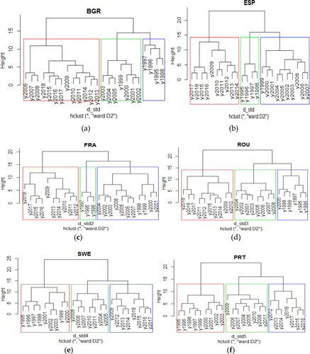
Using the clusters means vectors, centroids, obtained after applying k-means algorithm (that solution may differ from the clusters obtained by the Ward method) it can be identified and described each group. In order to have a better accuracy of the result and to minimize as much as possible the percentage of error in data collection, in the analysis we used standardized data, not raw data. For every country it is expected to be a class with low average values, one with high average values for indicators and another with values of indicators between the two classes. According to the signification of each category, one class represents a higher risk for recession, another a low risk and the last one represents the uncertainty about the recession risk or a moderate risk, in some cases. Also, in describing of each class, only the variables with the highest discriminative power are considered. The description for each country, considering the methodology presented above is as follows (Table 1 being the summary of the analysis):

Table 1. The synthesis of the main results using k-means algorithm for each country.

	Group name			Group structure
Country code	1	2	3	1	2	3
AUT	low	high	moderate	2004–2008, 2011	2009–2010, 2012–2018	1995–2003
BGR	low	moderate	high	2006–2018	1998–2005	1995–1997
BLR	high	moderate	low	1995–1996	2007–2018	1997–2006
CHE	high	low	moderate	1995–1999, 2001–2003	2000, 2010, 2004–2008	2009, 2011–2018
CZE	high	low	moderate	2001–2013	2014–2018	1995–2000
DEU	moderate	high	low	2006–2008, 2010–2012	1995–2005, 2009	2013–2018
DNK	low	high	moderate	1995–1999	2008–2015	2000–2007, 2016–2018
ESP	low	moderate	high	1995–1998	1999–2008	2009–2018
EST	low	high	moderate	2000–2005	1995–1999	2006–2018
FIN	moderate	high	low	2000, 2005–2008	2009–2018	1995–1999, 2001–2004
FRA	low	high	moderate	1995–1999	2009–2017	2000–2008, 2018
GBR	high	moderate	low	2008–2018	1999–2007	1995–1998
GRC	moderate	low	high	2000–2009	1995–1999	2010–2018
HUN	moderate	high	low	1999–2008	2009–2018	1995–1998
IRL	high	low	moderate	2008–2014	2015–2018	1995–2007
ISL	low	moderate	high	1995–2005	2006–2008, 2015–2018	2009–2014
ITA	moderate	low	high	1995–1999	2000–2008	2009–2018
LVA	high	moderate	low	1995–1999	2010–2018	2000–2009
NLD	moderate	high	low	2000–2010	2011–2018	1995–1999
NOR	high	low	moderate	2002–2004, 2009–2018	2000–2001, 2005–2008	1995–1999
POL	moderate	low	high	2000–2005	2006–2018	1995–1999
PRT	moderate	low	high	2013–2018	1995–2003	2004–2012
ROU	high	low	moderate	1995–2000	2001–2008	2009–2018
RUS	moderate	low	high	2007–2017	1999–2006, 2018	1995–1998
SVK	moderate	low	high	1995–2001	2002–2008, 2010–2012	2009, 2013–2018
SVN	low	moderate	high	2005–2008, 2017–2018	1995–2004	2009–2016
SWE	moderate	high	low	2005–2008	2009–2018	1995–2004
TUR	moderate	low	high	1995–2000	2001–2007	2008–2018
UKR	low	high	moderate	1999–2008	2009–2018	1995–1998

Source: Authors’ processing based on the output from R software.

In Austria, the first class, composed by period 2004–2008 and 2011 is characterized by high investments, moderate consumption, high growth and savings, moderate un-employment and high trade and moderate import and export. The second period of time, between 2012 and 2018 and 2009–2010, the economic indicators have decreased significantly, especially the investments, GDP growth, the unemployment rate was higher than in the first analysed class, so that the last economic crisis still show the effects. The third class presents the beginning of the analysed period from 1995 to 2003, when in Austria, the taxes and the interest payments were high, while the other indicators are low, in average.

In Bulgaria, from 2006 to 2018 it was a period characterized by high trade indicators, low general (both young and total) unemployment rate, and low inflation. Analysing the economic crisis, Bulgaria has a more pronounced ‘capacity for economic resilience’ (Oprea et al., 2020) than other Eastern Europe countries. Eight years before, between 1998 and 2005, the inflation was higher as well as the final consumption expenditure and unemployment, while savings were at the lowest point, in average. The beginning of the analysed period (1995–1997), in Bulgaria the inflation was at the highest level, while the trade, import, export and consumption expenditures were at the lowest point.

From 1995 to 1996, in Belarus the trade, import, export, savings were low, comparing with the next years, while the inflation, consumption and unemployment were high. The next several years, between 1997 and 2006 the GDP growth was higher, in average than the previously period, as well as trade, imports, exports. Between 2007 and 2018, the inflation and unemployment rates were at the lowest level comparing with the past years, but the growth was lower than the years before the crisis, as well as trade and consumption.

In Switzerland, between 1995–1999 and 2001–2003, the trade, imports, exports, GDP growth were low, while the consumption was high. The years before the economic crisis: 2000, 2004–2008 and in 2010, the inflation and GDP growth were high, while the trade was moderate. In the final analysed period, in 2009 and 2011–2018, the consumption and growth were low in average, while the unemployment rates, young and total, were high.

The analysis for Czech Republic reveals that between 2001 and 2013, the inflation, exports, imports, trade and savings had moderate values in average, while the unemployment was high. After 2014, the inflation and consumption were low, high investments and trade and low unemployment. Between 1995 and 2000, the inflation was at the highest level in average, as well as the final consumption, while the investments and trade were low.

In Germany, the periods 2006–2008 and 2010–2012 are characterized by high inflation, taxes on goods and services and GDP per capita growth. Before this period, between 1995 and 2005 and in 2009, the inflation was moderate in average, but the trade, exports, imports and GDP per capita growth were at the lowest level, while the unemployment was high. The last analysed period, between 2013 and 2018, the inflation was low, but the taxes and trade were high.

In Denmark, between 1995 and 1999, the taxes were relatively high, but the trade, imports and exports and savings were low. Between 2008 and 2015, the crisis increased (in average) the domestic credit to private sector by banks, trade, imports and exports. In this period the unemployment was very high, in average, especially for young people. In the years before the economic crisis and recently in 2000–2007 and 2016–2018, in Denmark, the consumption expenditures and unemployment reduced in average, but the savings increased.

Low import, export, trade, investments, but having a high GDP growth were characteristics for Spain between 1995 and 1998. The period for the next 10 years (1999–2008) can be described as low consumption and unemployment indicators and high investments, prices and savings. The last analysed decade (2009–2018) for Spain show, in average, high consumption, export, import, trade and unemployment, but low prices, savings and GDP growth.

For Estonia, between 1995 and 1999, the consumption and prices indicators were at the highest level, while the export, import and trade were moderate. The period 2006–2018 can be described as having (in average) the highest export, import and trade indicators and the lowest consumption and prices, while between 2000 and 2005, in Estonia the indicators regarding trade were at the lowest level, in average.

In Finland, between 2009 and 2018 the consumption and import were high, while the investments, GDP growth, export and savings and income were at the lowest level in average. The periods 1995–1999 and 2001–2004 are described as low import, but high unemployment indicators as well as the highest GDP growth. In 2000 and between 2005 and 2008 in Finland there was the lowest consumption level and the highest savings, trade and export averages for indicators.

Between 1995 and 1999 in France there was (in average) the highest GDP growth period with low import, trade, moderate savings and high unemployment. The period 2009–2017 is characterized by high consumption, import and trade and the lowest GDP growth, investments and savings. Between 2000 and 2008, and in 2018, the level of prices was the highest (in average), but the unemployment was the lowest.

In United Kingdom, the years between 1995 and 1998 can be described as a period with low consumption, export, import, and trade, but high GDP growth, savings and manufacture trade. Between 2008 and 2018, in UK were (in average) the lowest GDP growth, savings and the highest import, export, prices, trade and unemployment for young people. Between 1999 and 2007, the trade was at the highest level in average, while the unemployment was low.

The first analysed years (1995–1999) for Greece may be described as having the highest prices, export and GDP growth indicators and the lowest trade, import and unemployment in average. Between 2010 and 2018 is the second class described by the lowest GDP growth and prices and the highest consumption, trade, import and unemployment and after the crisis started, ‘Greece was severely affected as all of its regions more than doubled their rate of unemployment’ (Grekousis, 2018). The period between 2000 and 2009 is characterized by the lowest household consumption expenditures and unemployment and high GDP growth.

Between 1995 and 1998, in Hungary it was a period with high prices and low trade. Between 2009 and 2018 the consumption, prices were very low, while the import, trade and savings were very high in average. The last group of years, between 1999 and 2008, in Hungary was a moderate inflation, low savings, while the consumption was at the highest level. A recent study confirms that Hungary ‘had to overcome some truly deep fallback stages during the double-dip recession following the 2008 global crisis’ (Soreg & Bermudez-Gonzalez, 2021).

In Ireland, in period 1995–2007 the export, import, trade, investments and unemployment were at the lowest level, while prices and merchandise trade were high. Between 2008 and 2014, the GDP growth was very low (in average), while the unemployment and consumption were high. The last analysed years are characterized by a very low consumption, prices, very high GDP growth, export, investments and trade.

The situation in Island is similar to the pattern identified for other countries: 11 years (1995–2005) are characterized by high consumption and relatively high GDP growth and low export, import and trade. In 2006–2008 and between 2015 and 2018 the consumption was moderate as well as the import and export, while savings were high in average and the unemployment was low, while between 2009 and 2014, the GDP growth and gross savings were at the lowest level, and export, import, trade and unemployment were at the highest level in Island.

In Italy, the years between 1995 and 1999 the consumption, investments and external relations like: export, import and trade were at the lowest level in average, while the prices, unemployment and savings were high. Between 2000 and 2008, the investments were high, while the other indicators are between the first analysed years and the most recent period from analysis. Between 2009 and 2018, the consumption, export, import, unemployment, especially for young people and trade were high, while the prices, savings and investments were very low in average, comparing with other classes.

On the other side, in Latvia, the years between 1995 and 1999 are described by high consumption, prices and unemployment and low external relations as: import, export and trade, while in the following period from 2000 to 2009, the situation differs: lower consumption and unemployment indicators and high manufactures imports. A recent study regarding the economic crisis in Latvia shows that ‘the crisis was defined as an unfortunate event that hit the country hard from the outside’ (Nyblom et al., 2019). In 2010–2018 the situation changed and the import, export, trade, savings were high, while the inflation and consumption were low in average.

In Netherlands, the first years (1995–1999) are described as having high households’ consumption and GDP growth and low import, export, trade and moderate unemployment. Between 2011 and 2018, the export, import, savings, unemployment and trade were at the highest level, while the GDP growth and GDP per capita growth were at the lowest level. Between 2000 and 2010, in Netherlands, the taxes were high in average, while the unemployment was low.

Between 1995 and 1999, in Norway the consumption, export of goods and services, expressed by annual percent, GDP growth and unemployment were very high, while the export and savings were low. The periods 2002–2004 and 2009–2018 may be described by relatively low investments and low GDP growth and trade. Between 2000–2001 and 2005–2008, in Norway the consumption and unemployment were low, while the investments, savings and taxes were, in average, at the highest level.

The first five analysed years (1995–1999) for Poland may be described as having low export, import, investments and trade and high prices, gross savings and GDP growth. The next years, between 2000 and 2005 are defined, in average, by high consumption and unemployment and low savings. In the following period, between 2006 and 2018, in Po-land the consumption, prices and unemployment indicators are at the lowest level (in average), while the export, import, trade indicators are at the highest level.

On the other side, in Portugal, the first years (1995–2003) can be described as a period with low consumption, export, import, trade and unemployment indicators and high GDP growth, savings and inflation indicators. The following years (2004–2012) are the opposite of the first analysed years, with high consumption and the lowest savings and GDP growth indicators. Between 2013 and 2018 in Portugal, the export, import, trade, unemployment are high, while the prices are at the lowest level (in average).

In Romania, between 2001 and 2008, the export was low, while the GDP growth and investments were high. The last analysed years (2009–2018) show low consumption and prices and high export, import, savings and trade, in average. The first years (1995–2000) are defined in Romania by high consumption and inflation and low GDP growth, import, investments, unemployment, savings and trade indicators (in average).

The situation in Russia is not very different from the pattern for other European countries: the last years (between 2007 and 2017), the export, import, unemployment, prices and trade were low. Between 1999 and 2006 and in 2018, the consumption was low and the export, GDP growth, trade and savings were high in average. The first analysed years (1995–1998) are described by a very low GDP growth, investments and savings indicators and high consumption, prices and unemployment variables.

In Slovakia, between 1995 and 2001, the consumption, unemployment and prices were high, while the export, import, trade and investments were low. Between 2008 and 2010, the GDP growth and gross domestic savings indicators were high in average. Be-tween 2013 and 2018, in Slovakia, the final consumption expenditure, unemployment and GDP growth were low, while the export, import and trade indicators were high in average.

The situation in Slovenia is not very different: the first decade (1995–2004) is characterized by low import, export and trade and high prices, while between 2009 and 2016, the consumption, export, import and trade were relatively high in average, while the prices, investments and GDP growth were at the lowest level. The periods 2005–2008 and 2017–2018 are defined by a very low consumption and unemployment indicators and high GDP growth and savings. An analysis of debt and deficit growth rate shows that ‘in 2000–2012, Slovenia had a low general government debt before it began to grow above the recommended 60% of GDP’ (Paczoski et al., 2019).

In Sweden, the first decade (1995–2004) shows low export, import, trade, unemployment and savings indicators in average, and high investments and revenues indicators. Period 2005–2008, is described as having low consumption and high average values for investments, trade and savings, while in 2009 and 2018 the consumption, export, import and unemployment variables were relatively high, while the investments are low.

The period 2008–2018 in Turkey is characterized by having in average a low consumption and inflation and high import, investments, savings, unemployment and trade. Between 2001 and 2007, in Turkey the unemployment was relatively high in average, while between 1995 and 2000, the consumption and prices were at the highest level, while import, investments, unemployment, savings and trade were low.

In Ukraine, the first years from the analysed period (1995–1998) show low GDP growth, import and the domestic credit to private sector by banks, and trade and very high prices. Between 2009 and 2018, the consumption, import and trade in services were high, while the inflation and savings indicators were low. Between 1999 and 2008, the consumption was low, while the export, GDP growth, trade and savings variables were high in average.

The individual study of each country reveals a pattern regarding the analysis of each of the three classes and show two major periods of discontinuance: one period between 1998 and 2000 and another between 2008 and 2010. Each period corresponds to a significant period of crisis: the year 1997, the Asian crisis that affected the European countries, and the 1998 corresponds to the Russian financial crisis, ‘that was initially started by the Asian crisis that led to a decrease of raw materials prices’ (Pribac, 2011) and in 2008–2009 the most recent financial crisis that affected all European countries, some were affected more while other were affected less. These variations in time are visible for each country when the class of recession risk changes. It can be observed that there are many changes from moderate risk of recession to high risk of recession in 2008–2010 (as Figure 2 shows).

Figure 2. Classes’ evolution for European countries.

Source: Authors’ processing based on the output from R software.

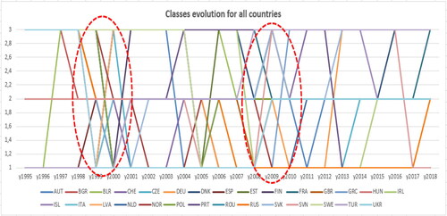
In Figure 2 from above it is shown, for each country, how varies the class for recession risk in the analysed period of time. Two major areas that represent disturbances regarding the change of the classification class and also, that represent changes in macroeconomic indicators are: between 1998 and 2000 and between 2008 and 2010, even thou each country has its own rhythm of economic growth and its own cyclicality of economic cycles. Figure 2 shows that in the last seven years from the analysed period, since 2012 to 2018, only few countries changed the class of recession risk, comparing with the period between the two major class changing periods, 2001–2007. Taking into consideration the value, in average, for growth and money indicators, as well as all other indicators with significant discriminative power, each class correspond to a level of recession risk: low recession risk, moderate risk or high recession risk. The main results regarding the signification of each group of years specifically for each country and the years that represents each class may be found in Table 1. The synthesis of the main results using k-means algorithm for each country

Another way to visualize the discontinuances in time regarding the risk of recession representing the class of recession risk as coloured maps, each colour is in according to the associated class of each country.

Figure 3 shows the evolution of class and the comparison of major discontinuances in time regarding the evolution of the recession risk. The name of recession risk class is established using the class centres, measured as an average value, as mentioned above. Each class in each country has its own particularities. The first two images (a and b) show the comparison between 1998 and 2000 and the impact of Asian and Russian crises which are visible in the evolution of recession risk: some countries were less affected by these crises and other changed the risk from low to moderate, having a higher impact. The next two figures (c and d) show the impact of the economic crisis that started in 2009: the comparison between 2008 and 2010 maps shows that the impact of this crisis was very strong. It can be observed that the map is almost entire coloured in dark blue colour which is representing the class with high recession risk. The last two maps (e and f) show the beginning of the analysed period, year 1995, and the final studied year, 2018.

Figure 3. Recession risk in time: (a) 1998; (b) 2000; (c) 2008; (d) 2010; (e) 1995; (f) 2018.

Source: Outputs obtained in R software.

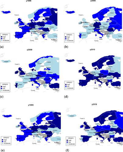
Taking into account the maps presented in Figure 3 and the centroids analysis it can be concluded that each country has its own evolution rhythm of economic cycles. But, in case of an economic crisis, like the one which started in 2008, that affects the entire economies, the effects are visible in most European countries, and only few of them resist to high recession risk. Some of the European countries needed long time to recover from the last crisis started in 2008, like Greece or Spain that had a negative GDP per capita growth since 2008 to 2013.

Thus, globally, two major periods have been identified in the economies of European countries in which there have been changes in the recession risk class (Figure 2). The observed distance between the beginnings of these periods is 9–10 years, which means that the next period where major changes will be observed will be 2019–2020. Moreover, from the graphical analysis of the evolutions of the recession risk classes, it is observed that the situation at the end of the analysis period, in 2018, is one in which many states have an increased risk of recession. This fact is also supported by the macroeconomic situation by the worsening of the main indicators compared to previous years.

5. Conclusions

Over time, humanity has gone through several high risk of economic crises, crises that began as a result of more or less predictable events. The main concern has always been to try to prevent hazard and to have predictability so that, through the measures adopted in time, to limit as much as possible the effects of periods of economic recession. Thus, special algorithms in the field of econometrics, data analysis and even artificial intelligence were used to find hidden information, difficult to detect at first sight. From the analysis made in this scientific paper, two economically critical situations are identified at the level of the European continent: in 1998–1999 and in 2008–2009. Each of these periods had a different starting point: the financial crisis of 1998 and the economic crisis in 2009. Due to the close economic and financial relations between states, globally, a crisis that initially begins and manifests itself outside the European space has undoubted effects on European countries. The limitations of this study mainly refer to the fact that by analysing the components of a large system it is possible to predict the behaviour of the whole system. Each economic subsystem has its own economic policy and each reacts differently to a crisis. Therefore, there are other methods for more accurately predicting the next crisis with effects at European level, such as econometric approaches, like regression, time series or applying the Markov chains, which provide a different perspective on this issue and could represent further research. A possible extension for this research represents the study of the hazard that appeared in 2020 with the sanitary crisis, a situation that could have the effect of accelerating a potential economic crisis in Europe. Several studies already recommend measures to reduce the impact of an economic crisis, like: ‘the redesign of economic policies at European level’ (Soava et al., 2020), ‘substantial reforms in European pension and unemployment insurance systems’ (Briceño & Perote, 2020), or identify different effects of pandemic in economy, like ‘banking sector liquidity increased, the profitability and solvency decreased’ (Teresienė et al., 2021) or suggest that ‘countries need to take measures to mitigate the economic effects’ for the economic crisis caused by Covid-19 (Oravský et al., 2020).

Disclosure statement

No potential conflict of interest was reported by the authors.

References

- Aghabozorgi, S., Shirkhorshidi, A. S., & Wah, T. Y. (2015). Time-series clustering – A decade review. Information Systems, 53, 16–38. https://doi.org/10.1016/j.is.2015.04.007
- Alaminos, D., Peláez, J. I., Salas, M. B., & Fernández-Gámez, M. A. (2021). Sovereign debt and currency crises prediction models using machine learning techniques. Symmetry, 13(4), 652. https://doi.org/10.3390/sym13040652
- Augustyński, I., & Laskoś-Grabowski, P. (2018). Clustering macroeconomic time series, econometrics. Econometrics, 22(2), 74–88. https://doi.org/10.15611/eada.2018.2.06
- Briceño, H. R., & Perote, J. (2020). Determinants of the public debt in the eurozone and its sustainability amid the Covid-19 pandemic. Sustainability, 12(16), 6456. https://doi.org/10.3390/su12166456
- Brkić, I., Gradojević, N., & Ignjatijević, S. (2020). The impact of economic freedom on economic growth? New European dynamic panel evidence. Journal of Risk and Financial Management, 13(2), 26. https://doi.org/10.3390/jrfm13020026
- Clift, B. (2020). The IMF, the Eurozone and global financial crises, and the politics of economic ideas. Comparative European Politics, 18(1), 99–108. https://doi.org/10.1057/s41295-018-0146-x
- Danko, J., & Suchý, E. (2021). The financial integration in the european capital market using a clustering approach on financial data. Economies, 9(2), 89. https://doi.org/10.3390/economies9020089
- Dinçer, H., Yüksel, S., & Şenel, S. (2018). Analyzing the global risks for the financial crisis after the great depression using comparative hybrid hesitant fuzzy decision-making models: Policy recommendations for sustainable economic growth. Sustainability, 10(9), 3126. https://doi.org/10.3390/su10093126
- Grekousis, G. (2018). Further widening or bridging the gap? A cross-regional study of unemployment across the EU amid economic crisis. Sustainability, 10(6), 1702. https://doi.org/10.3390/su10061702
- Iuga, I. C., & Mihalciuc, A. (2020). Major crises of the XXIst century and impact on economic growth. Sustainability, 12(22), 9373. https://doi.org/10.3390/su12229373
- Liao, Y. (2017). Machine learning in macro-economic series forecasting. International Journal of Economics and Finance, 9(12), 71–76. https://doi.org/10.5539/ijef.v9n12p71
- Michie, J. (2020). Analysing economic crises, and creating a new era of sustainable development. International Review of Applied Economics, 34(1), 1–3. https://doi.org/10.1080/02692171.2020.1672985
- Ntanos, S., Skordoulis, M., Kyriakopoulos, G., Arabatzis, G., Chalikias, M., Galatsidas, S., Batzios, A., & Katsarou, A. (2018). Renewable energy and economic growth: Evidence from European countries. Sustainability, 10(8), 2626. https://doi.org/10.3390/su10082626
- Nyblom, Å., Isaksson, K., Sanctuary, M., Fransolet, A., & Stigson, P. (2019). Governance and degrowth. lessons from the 2008 Financial crisis in Latvia and Iceland. Sustainability, 11(6), 1734. https://doi.org/10.3390/su11061734
- Oprea, F., Onofrei, M., Lupu, D., Vintila, G., & Paraschiv, G. (2020). The determinants of economic resilience. The case of Eastern European regions. Sustainability, 12(10), 4228. https://doi.org/10.3390/su12104228
- Oravský, R., Tóth, P., & Bánociová, A. (2020). The ability of selected European countries to face the impending economic crisis caused by COVID-19 in the context of the global economic crisis of 2008. Journal of Risk and Financial Management, 13(8), 179. https://doi.org/10.3390/jrfm13080179
- Paczoski, A., Abebe, S. T., & Cirella, G. T. (2019). Debt and deficit growth rate reporting for post-communist European Union member states. Social Sciences, 8(6), 173. https://doi.org/10.3390/socsci8060173
- Pribac, L. I. (2011). Scurt istoric al crizelor economice mondiale din secolul XX pana in present. Investitiile - Solutia anticriza pentru Romania [Brief history of world economic crises from the twentieth century to the present. Investments - Anti-crisis solution for Romania]. Studia Universitatis Vasile Goldis Arad, 2011, Seria Stiinte Economice, 21.
- Soava, G., Mehedintu, A., Sterpu, M., & Raduteanu, M. (2020). Impact of employed labor force, investment, and remittances on economic growth in EU countries. Sustainability, 12(23), 10141. https://doi.org/10.3390/su122310141
- Soreg, K., & Bermudez-Gonzalez, G. (2021). Measuring the socioeconomic development of selected balkan countries and hungary: A comparative analysis for sustainable growth. Sustainability, 13(2), 736. https://doi.org/10.3390/su13020736
- Teresienė, D., Keliuotytė-Staniulėnienė, G., & Kanapickienė, R. (2021). Sustainable economic growth support through credit transmission channel and financial stability: In the context of the COVID-19 pandemic. Sustainability, 13(5), 2692. https://doi.org/10.3390/su13052692
- The World Bank. ( n.d.). https://data.worldbank.org/indicator
- Vo, V., Luo, J., & Vo, B. (2016). Time series trend analysis based on k-means and support vector machine. Comput. Informatics, 35, 111–127.