Dynamic characteristics of China's inflation: a two-country DSGE model based on a multi-level vertical industrial structure

Abstract

We establish a two-country DSGE model with a vertical production chain to study the inflation dynamics in China. By introducing multiple layers of price stickiness and shadow economy production to the vertical industrial chain, our model helps to explain dynamic characteristics of inflation. In our model, shocks can not only affect inflations by passing down the production chain through cost channels, but also in the reverse way due to the intermediate demand effect and the investment costs effects. After calibrating and estimating the parameters, the simulation results show that more than 90% of inflation fluctuations in China can be attributed to domestic shocks, among which the domestic monetary shock and final sector technology shock are the most influencing factors in explaining China’s inflation dynamics.

Keywords:

• Inflation
• vertical industry chain
• multi-layer price stickiness
• DSGE modelling

JEL Classifications:

• C61
• E31
• F41

1. Introduction

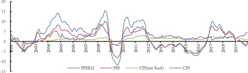
The acceleration of market reform and globalization has a huge impact on China’s economic performance, especially on inflation. Using the Primary Price Index of Raw Material (PPIRM), Producer Price Index (PPI) and non-food Consumer Price Index to measure China's inflation, Figure 1 shows that China’s inflation has shown obvious cyclicality: all inflation indicators change simultaneously. Moreover, inflation volatility differs in magnitude: PPIRM has the largest fluctuation, PPI has moderate volatility, and CPI shows stronger smoothness than PPIRM and PPI.

Figure 1. China’s inflation index since 2001.

Data source: Wind database.

In order to characterize the characteristics of China's inflation, we try to construct a two-country DSGE model with three-layer production chain, the upper, middle and lower productions, to study the dynamic characteristics and transmission mechanism of China's inflation. In the model, the upper, middle and lower industries correspond to the production of ‘primary goods’, ‘industrial goods’ and ‘final (consumer) goods’ production.¹ Moreover, we introduce Calvo (1983) price adjustments into each layer of the vertical industrial chain; therefore, the setting of multi-layer price stickiness produces stronger inflation smoothness. Besides, by incorporating the shadow economy, the interaction of shadow economy with production chain in the model provides a better explanation to the real economy.

We use quarterly data of China and the United States to calibrate and estimate the parameters, and compare the impact of technology shock, investment shock, consumption and monetary policy shocks. Our conclusion shows that the introduction of vertical industrial chain and multi-layer price stickiness reduces the impact of upper-layer production shock, while technology and investment shocks from lower-layer not only produce the most obvious impact on CPI, more importantly, these shocks will be transmitted to the upper layer production, influencing PPI and PPIRM. The impulse response and counterfactual simulations also confirm that our model’s results are much closer to China’s reality than the standard NK models.

This article mainly contributes to the literature by introducing of vertical the industrial chain in the model, which exhibits more complicated inflation transmission mechanisms. Specifically, because the price stickiness in the model is imposed on each layer, shocks from the upper layer of the industrial chain are more smoothed out. More importantly, inflation in our model can be passed not only from the top layer of the production chain to bottom through cost channels, but also from the bottom layer to top through both intermediate products demand effect and the investment price effect. In our model, the former is a relatively weak channel. For example, a positive technology shock from the industrial goods sector leads to a decline in PPI, which is its direct effect. However, the decline in PPI will bring about more consumption of industrial intermediate products in the final production, which partly offsets the decline in PPI. Compared with the demand mechanism, the price effect of investment goods is more obvious, since all sectors use final products as investment. Therefore, the shocks from final goods production will directly affect the cost of all sectors.

Another contribution of this article is that, in each layer of the production chain, we introduce shadow economy production, which has lower costs than the formal economy. Since the middle and upper layers of the industrial chain are more controlled by state-owned enterprises in China, our model sets a larger proportion of the informal economy at the lower layer of the industrial chain. Under this setting, our model highlights interactions of shadow economy and industrial production chain in explaining inflation smoothness.

The remainder of this article is structured as follows. Section 2 reviews the relevant literature. Section 3 provides an overview of the model, a two-country DSGE model with vertical industrial chains of upper, middle and lower productions. Section 4 reports the parameter calibration and prior distribution, as well as the Bayesian estimation results. Based on that, Section 5 decomposes the influencing factors of China’s inflation and compares the contribution of technological shock, monetary shock, preference and investment shocks from domestic and abroad. In Section 6, we present the IRFs, and by constructing counterfactual simulations without multilevel industry and no shadow economy production, we verify the role of vertical industrial chain and shadow economy in smoothing China's inflation. Finally, Section 7 concludes.

2. Literature review

Research on the dynamic characteristics of inflation has always been the core of macroeconomics. In the 1990s, Gali and Gertler (1999), Clarida et al. (1999) analyse the Phillips in the framework of New Keynesian economics, but it is still difficult to explain the persistence of the actual inflation due to the model’s completely forward-looking characteristics. In order to reconcile the theoretical and the empirical results, Christiano et al. (2005) propose a more general inflation dynamic model, that is, the hybrid new Keynesian Phillips Curve (HNKPC). Although the HNKPC model responds to the challenge of the inflation persistence relatively well, Rudd et al. (2005) and Rudd and Whelan (2006) find that its improvement is mainly due to the introduction of lagging inflation, which is sharply criticized for it is arbitrarily introduced into the model.

To give a firm explanation to inflation dynamics, the analysis of inflation and monetary policy from the perspective of industrial structure has attracted more and more academic attention. Horvath (2000), Kim and Kim (2006) use the industrial input-output table to construct a model with production structure, and their results show that integrating the input-output structure makes the model fit the inflation fluctuation well, without resorting to large total shocks. Huang and Liu (2007) and Wong and Eng (2010) use the industrial structure model to analyse the transmission of inflation shocks, in their models, multi-layer price staggered adjustment strengthens price stickiness. Carvalho et al. (2021) compare the impact of aggregate and sectoral shocks on inflations and verifies that under the input-output structure, inflation responds more slowly to aggregate shocks, but more quickly to sectoral shocks. Moro (2012) and Pinto (2021) make cross-country studies on industrial structure and economic volatility. In their studies, the intensification of the industrial structure and the increase in the proportion of service sector leads to the stability of economic fluctuations. Bouakez, (2022) finds that the shock from the upper-layer industry will be gradually weakened through the cost channel, while the lower-layer impact has a stronger effect on prices and output.

On the topic of inflation dynamics in China, though the most studies are mostly based on empirical analysis (Chow & Wang, 2010; Funke et al., 2015), some recent literatures start to analyse in more theoretical ways. Some studies use DSGE models and dynamic econometrics to estimate the New Keynesian Phillips Curve (Li et al., 2015; He et al., 2017). However, this type of literature often requires the exogenous assumptions of the backward pricing, and ignores the influence of production structure.

Our research is based on the model of Huang and Liu (2007),Wong and Eng (2010) and Bouakez et al. (2022). Compared with literatures such as Huang and Liu (2007) and Wong and Eng (2010), our model includes not only technical shock, but also investment shock, monetary and preference shocks. More importantly, in our model shocks can not only pass along the industrial chain from top layer to bottom, there is also a reverse transmission mechanism including both the investment price effect and intermediate products demand effect. Therefore, by introducing vertical industrial structure, this article enriches the dynamic mechanisms of inflation.

Second, we consider the existence of informal economies in China. The literature of shadow economy also helps to understand the inflation dynamics, especially for developing countries. Solis-Garcia and Xie (2018) use a two-sector general equilibrium model to discuss the output volatility of shadow economy. Colombo et al. (2016) investigate the response of shadow economy to economic crisis, and concludes that the informal sector is a powerful buffer, which absorbs a large proportion of the fall in official output. By incorporating the informal economy, our model produces further smoothness of inflation.

Finally, compared to the existing literature, our open economy setting is more realistic. Bouakez et al. (2022) provide an explicit solution to the multi-layer industrial structure model, but their model does not introduce an open economy. The studies of Huang and Liu (2007) and Wong and Eng (2010) all stay on the assumption that the economies of the two countries are completely symmetrical and the production along industrial chains are completely the same. Besides, they use parameter calibration methods for numerical simulation analysis, which makes it difficult to draw conclusions that reflect the characteristics of the two countries. In contrast, we combine calibration and estimation methods and use actual data from China and the United States to determine the parameters. Therefore, our model is more in line with the actual situation of China and the United States in terms of economic scale and industrial structure.

3. The model

We introduce the vertical input-output structure of production into the two-country model. It is assumed that the world is composed of two countries, where country $H$ is domestic (such as China) and country $F$ is foreign (such as the United States).² Due to the vertical production structure, in each country, the production problems are conducted by primary, industrial, and final goods entrepreneurs.

3.1. Households

Representative households in country $H$ obtain utility through consumption $C_t,$ actual currency holdings $m_t,$ where $m_t=M_t/P_{3,t},$ and leisure. The domestic representative family’s utility function is given by (1) $$U=\sum _{t=0}^{\infty }{\beta }_{}^t{\varsigma }_t\left[\frac{{\left(C_t\right)}^{1-\sigma }}{1-\sigma }+\frac{{\left(M_t/P_{3,t}\right)}^{1-\psi }}{1-\psi }-\frac{{\left(L_t\right)}^{1+\upsilon }}{1+\upsilon }\right]$$(1) subject to the budget constraints (2) $$\begin{array}{c}{P}_{3,t}{C}_t+P_{I,t}{I}_t+M_t+\sum _{v_{t+1}}Q\left(v_{t+1}|v_t\right)B_{H,t+1}\left(v_{t+1}\right)\\ +S_t\sum _{v_{t+1}}{Q}^F\left(v_{t+1}|v_t\right)B_{F,t+1}^{}\left(v_{t+1}\right)\\ =W_t{L}_t+M_{t-1}+B_{H,t}+B_{F,t}^{}+T_t+P_{3,t}{\Theta }_t+R_{K,t}{K}_t\end{array}$$(2) where $\beta$ is the time discount factor and $L_t$ denotes labour. $M_t$ measures the amount of money held by consumers and $P_{3,t}$ denotes the overall domestic consumer price level. ${\varsigma }_t$ represents the exogenous consumer preference shock. $B_{H,t+1}(v_{t+1})$ and $B_{F,t+1}^{}(v_{t+1}),$ respectively, denote that in state $v_{t+1},$ the family can get $B_{H,t+1}$ units of local currency income and $B_{F,t+1}^{}$ units of foreign currency income. $Q$ and $Q^F$ represent the corresponding bond prices. $I_t$ is the actual investment, $T_t$ is the one-time transfer payment from the government, $P_{I,t}$ is the price of the investment product, $W_t$ is the nominal wage, $S_t$ represents the nominal exchange rate, $R_{K,t}{K}_t$ is the investment income, and $P_{3,t}{\Theta }_t$ is the profit from the enterprise.

It is worth noting that the consumption of representative domestic households $C_t$ is composed of domestic products $C_{3H,t}$ and imported products $C_{3F,t}:$ (3) $$C_t={\left[{\left(1-a_H\right)}^{1/\epsilon }{\left(C_{3H,t}\right)}^{1-1/\epsilon }+a_H^{1/\epsilon }{\left(C_{3F,t}\right)}^{1-1/\epsilon }\right]}^{\epsilon /\left(\epsilon -1\right)}$$(3) where $a_H$ is the foreign consumer goods preference coefficient and $\epsilon$ is the consumption substitution elasticity of the two products.Similarly, actual investment $I_t$ consists of domestic investment goods $I_{H,t}$ and imported investment goods $I_{F,t},$ that is (4) $$I_t={\left[{\left(1-a_I\right)}^{1/{\epsilon }_I}{\left(I_{H,t}\right)}^{1-1/{\epsilon }_I}+a_I^{1/{\epsilon }_I}{\left(I_{F,t}\right)}^{1-1/{\epsilon }_I}\right]}^{{\epsilon }_I/\left({\epsilon }_I-1\right)}$$(4) where $a_I$ is the preference coefficient of foreign investment products and ${\epsilon }_I$ is the substitution elasticity of the two investment products. Given the investment level $I_t,$ the household’s capital accumulation equation is given by (5) $$K_{t+1}=\left(1-\delta \right)K_t+{\xi }_t\left[1-\Gamma \left(I_t/I_{t-1}\right)\right]I_t$$(5) where $\Gamma (I_t/I_{t-1})I_t$ is the investment adjustment cost, assuming that $\Gamma (1)={\Gamma }^{\prime }(1)=0$ at steady state and ${\Gamma }^{″}(1)>0.$ ${\xi }_t$ represents investment shock.

3.2. Primary product production and primary product price index

We assume that the primary product producers in country $H$ are monopolistic competitive enterprises distributed in the continuum$\left[0,1\right],$ among which, the proportion of the shadow economy is ${\varpi }_{1H},$ and the proportion of 1-${\varpi }_{1H}$ is the formal economy. It is further assumed that both the formal and shadow economies are operated by enterprises, who use capital and labour factors in production. As far as the formal economy is concerned, the production function of representative manufacturer is given by (6) $$Y_{1,t}=A_{1,t}{K}_{1,t}^{{\alpha }_1}{L}_{1,t}^{1-{\alpha }_1}$$(6) where $A_{1,t}$ represents the technical level of primary goods production. $K_{1,t}^{}$ and $L_{1,t}^{}$ represent the amount of capital and labour input in the production of primary goods. For the shadow economy, we assume its technology shows decreasing return to scale, and its production function is $$Y_{1,t}=A_{1,t}{K}_{1,t}^{\tau {\alpha }_1}{L}_{1,t}^{\tau (1-{\alpha }_1)}$$ where $\tau$ is a parameter less than 1.

We adopt the sticky pricing method of Calvo (1983), that is, enterprises choose optimal price ${\tilde{P}}_{1H,t}$ with probability $1-{\theta }_1$ per period, or otherwise prices remain unchanged. Then, we obtain the inflation dynamics of primary products: (7) $$\begin{array}{c}{\pi }_{1H,t}={\varpi }_{1H}{\pi }_{1H\_1,t}+\left(1-{\varpi }_{1H}\right){\pi }_{1H2,t}\\ =\beta E_t{\pi }_{1H,t+1}+\frac{\left(1-\theta \right)\left(1-\beta \theta \right)}{\theta }\left\{\right[1+{\varpi }_{1H}(\tau -1)]\\ [\left(1-{\alpha }_1\right){\widehat{w}}_t+{\alpha }_1{\widehat{r}}_{K,t}]-{\widehat{A}}_{1,t}+{\widehat{P}}_{3,t}-{\widehat{P}}_{1H,t}\}.\end{array}$$(7)

In the above equation, since $\tau$ is a parameter less than 1, the larger of the shadow economy’s fraction ${\varpi }_{1H},$ the more it will offset the changes in marginal cost, making primary product inflation show more smoothness.

Furthermore, we assume that the primary products $Y_{1H,t}$ and $Y_{1F,t}$ from home and abroad are used for industrial production as primary intermediate inputs $Z_{1,t},$ which takes the form (8) $$Z_{1,t}={\left[{\left(1-{\kappa }_1\right)}^{1/{\phi }_1}{\left(Y_{1H,t}\right)}^{1-1/{\phi }_1}+{\kappa }_1^{1/{\phi }_1}{\left(Y_{1F,t}\right)}^{1-1/{\phi }_1}\right]}^{{\phi }_1/\left({\phi }_1-1\right)}$$(8) where ${\kappa }_1$ is a parameter reflecting the degree of participating in the international production chain. If ${\kappa }_1=0,$ the model degenerates into the basic two-country DSGE, in which each country uses only domestic factors for production. Given the prices of primary goods in both countries {$P_{1H,t}^{},$$P_{1F,t}^{}$}, we can easily find the price index of the production of primary goods in country $H$ is (9) $$P_{1,t}={\left[\left(1-{\kappa }_1\right)P_{1H,t}^{1-{\phi }_1}+{\kappa }_1{P}_{1F,t}^{1-{\phi }_1}\right]}^{1/\left(1-{\phi }_1\right)}$$(9)

3.3. Industrial production and industrial price index

For the middle production layer, we assume that the industrial product manufacturing enterprises in country $H$ are monopolistic competitive enterprises distributed in the continuum$\left[0,1\right],$ and the proportion of the shadow economy is ${\varpi }_{2H}.$ As for the formal economy, it uses primary composite products $Z_{1,t}$ as well as domestic labour and capital factors in production. Its production function is given by (10) $$Y_{2,t}=A_{2,t}{Z}_{1,t}^{{\chi }_1}{\left(K_{2,t}^{{\alpha }_2}{L}_{2,t}^{1-{\alpha }_2}\right)}^{1-{\chi }_1}$$(10) where $A_{2,t}$ represents the technology level in industrial production. Similarly, we set the industrial production function of shadow economy as $$Y_{2,t}=A_{2,t}{Z}_{1,t}^{{\chi }_1}{\left(K_{2,t}^{\tau {\alpha }_2}{L}_{2,t}^{\tau (1-{\alpha }_2)}\right)}^{1-{\chi }_1}$$ where $\tau$ is a parameter less than 1. In price setting, we also assume that the enterprise chooses the optimal price ${\tilde{P}}_{2H,t}$ with probability $1-{\theta }_2$ in each period, and otherwise the price remains unchanged. Based on the Phillips curve of two types of enterprises, the dynamic inflation equation of industrial products can be obtained to satisfy (11) $$\begin{array}{c}{\pi }_{2H,t}=\beta E_t{\pi }_{2H,t+1}+\frac{\left(1-{\theta }_2\right)\left(1-\beta {\theta }_2\right)}{{\theta }_2}\\ \left([1+{\varpi }_{2H}(\tau -1)][\left(1-{\alpha }_2\right){\widehat{w}}_t+{\alpha }_2{\widehat{r}}_{K,t}]-{\widehat{A}}_{2,t}+{\widehat{P}}_{3,t}-{\widehat{P}}_{2H,t}\right)\end{array}$$(11)

In the above equation, a larger ${\varpi }_{2H},$ which means higher share of the shadow economy, produces more smoothness of the industrial products’ inflation.

Similarly, we assume {$Y_{2H,t}^{},$$Y_{2F,t}^{}$} are used for the production of final products as industrial intermediate inputs $Z_{2,t},$ which takes the form of (12) $$Z_{2,t}={\left[{\left(1-{\kappa }_2\right)}^{1/{\phi }_2}{Y}_{2H,t}^{1-1/{\phi }_2}+{\kappa }_2^{1/{\phi }_2}{Y}_{2F,t}^{1-1/{\phi }_2}\right]}^{{\phi }_2/\left({\phi }_2-1\right)}$$(12) where ${\kappa }_2$ is the share of foreign industrial products. Given the industrial products prices of the two countries {$P_{2H,t}^{},$$P_{2F,t}^{}$}, we can easily calculate the industrial product price index of country $H.$ (13) $$P_{2,t}={\left[\left(1-{\kappa }_2\right)P_{2H,t}^{1-{\phi }_2}+{\kappa }_2{P}_{2F,t}^{1-{\phi }_2}\right]}^{1/\left(1-{\phi }_2\right)}$$(13)

3.4. Final goods production and consumer price index

As the settings of the previous part, we assume that the proportion of the shadow economy in the production of industrial products is ${\varpi }_{3H},$ and the ratio 1-${\varpi }_{3H}$ is the share of formal economy. As for the latter, its production function is (14) $$Y_{3,t}=A_{3,t}{Z}_{2,t}^{{\chi }_2}{\left(K_{3,t}^{{\alpha }_3}{L}_{3,t}^{1-{\alpha }_3}\right)}^{1-{\chi }_2}$$(14) where $Z_{2,t}$ is the industrial composite used in final goods production, $A_{3,t}$ represents its technology level.

Entrepreneurs from both economies choose the optimal price ${\tilde{P}}_{3H,t}$ with probability $1-{\theta }_3$ every period, and otherwise the price remains unchanged. Therefore, the dynamic price equation of final products can be obtained as (15) $${\pi }_{3H,t}=\beta E_t{\pi }_{3H,t+1}+\frac{\left(1-{\theta }_3\right)\left(1-\beta {\theta }_3\right)}{{\theta }_3}\left([1+{\varpi }_{3H}(\tau -1)][\left(1-{\alpha }_3\right){\widehat{w}}_t+{\alpha }_3{\widehat{r}}_{K,t}]-{\widehat{A}}_{3,t}+{\widehat{P}}_{3,t}-{\widehat{P}}_{3H,t}\right)$$(15)

Given the price of consumer goods $P_{3H,t}$ in country $H$ and the import price of consumer goods $P_{3F,t}$ in country $F,$ we can get the consumer price index in country $H.$ (16) $$P_{3,t}={\left[\left(1-a_H\right){\left(P_{3H,t}\right)}^{1-\epsilon }+a_H{\left(P_{3F,t}\right)}^{1-\epsilon }\right]}^{1/\left(1-\epsilon \right)}$$(16)

3.5. International trade

The international trade in our model not only reflects the trade of three intermediate goods in the production chain, but also reflects the trade of final goods used for consumption and investment. Net exports of primary products $n{x}_{1,t}$ and net exports of industrial products $n{x}_{2,t}$ are $$n{x}_{1,t}=\left(P_{1H,t}^{}{Y}_{1H,t}^F-P_{1F,t}{Y}_{1F,t}\right)/P_{3,t},n{x}_{2,t}=\left(P_{2H,t}^{}{Y}_{2H,t}^F-P_{2F,t}{Y}_{2F,t}\right)/P_{3,t}$$

The final product export is composed of net exports of consumer goods $n{x}_{3,t}$ and investment goods $n{x}_{4,t},$ which are, respectively, given by $$n{x}_{3,t}=\left(P_{3H,t}^{}{C}_{3H,t}^F-P_{3F,t}^{}{C}_{3F,t}\right)/P_{3,t},n{x}_{4,t}=\left(P_{3H,t}^{}{I}_{H,t}^F-P_{3F,t}^{}{I}_{F,t}\right)/P_{3,t}$$

The total net export of country $H$ is $n{x}_t=n{x}_{1,t}+n{x}_{2,t}+n{x}_{3,t}+n{x}_{4,t}.$

3.6. Monetary policy and shocks

We assume the domestic monetary policy to follow Taylor rules with the following form (17) $${\widehat{R}}_t={\rho }_R^{}{\widehat{R}}_{t-1}^{}+{\rho }_Y{\widehat{Y}}_t+{\rho }_{\pi }{\widehat{\pi }}_{3,t}+{\xi }_{\text{mpe},t}^{}$$(17) where ${\widehat{R}}_t$ represents the domestic interest rate level, ${\widehat{Y}}_t$ represents the domestic output gap, ${\widehat{\pi }}_{3,t}$ is the domestic inflation gap measured by the consumer price index, ${\rho }_R^{}$ is a parameter measuring the lag effect of domestic monetary policy, ${\rho }_Y$ and${\rho }_{\pi }$ are parameters reflecting how the domestic monetary policy depends on the output gap and inflation gap. ${\xi }_{\text{mpe},t}^{}$ represents domestic monetary policy shock. Similarly, the monetary policy of country $F$ is (18) $${\widehat{R}}_t^F={\rho }_R^F{\widehat{R}}_{t-1}^F+{\rho }_Y^F{\widehat{Y}}_{3,t}^F+{\rho }_{\pi }^F{\widehat{\pi }}_{3,t}^F+{\xi }_{\mathit{mpe},t}^F$$(18)

In addition, there are three types of exogenous shocks in our model: technology shocks {$A_{1,t},$$A_{2,t},$$A_{3,t},$$A_{1,t}^F,$$A_{2,t}^F,$$A_{3,t}^F$}, consumption shocks {${\varsigma }_t,$${\varsigma }_t^F$}, investment shocks {${\xi }_t,$${\xi }_t^F$}. We assume that all exogenous shocks satisfy the process of AR (1):${\vartheta }_t={\rho }_{\vartheta }{\vartheta }_{t-1}+{\epsilon }_t^{\vartheta }.$

4. Parameter calibration and estimation

4.1. Parameter calibration

We use parameter calibration and Bayesian estimation to set parameter values. We calibrate parameters according to China’s macroeconomic data from 1995 to 2019 (see Table 1). The specific settings are as follows.

Table 1. Parameter calibration.

${\beta }^H$	${\beta }^F$	${\sigma }^H$	${\sigma }^F$	$\upsilon$	$\delta$	${\alpha }_1$	${\alpha }_2$	${\alpha }_3$	${\mu }_1$	${\mu }_2$	${\mu }_3$	${\chi }_1$
0.99	0.997	1.5	2	1	0.025	1/3	1/3	1/3	1.1	1.1	1.1	0.67
${\chi }_2$	$a_H$	$a_I$	$a_F$	$a_I^F$	${\kappa }_1$	${\kappa }_1^F$	${\kappa }_2$	${\kappa }_2^F$	$\epsilon$	${\epsilon }_I$	${\phi }_1$	${\phi }_2$
0.67	0.1	0.1	0.12	0.12	0.45	0.3	0.45	0.3	2	2	1	1

Source: Authors.

Country $H$ represents China and country $F$ represents the United States. As for China, we set $\beta =0.99$ so that the annual risk-free interest rate is 4%, generally, in line with China's one-year deposit interest rate. For the United States, taking into account the long-term low interest rates, set ${\beta }^F=0.997,$ so that the annualized risk-free interest rate is 1%. Referring to Devereux et al. (2006), we set the reciprocal of the risk aversion coefficient in the United States ${\sigma }^F=2,$ while China is lower ${\sigma }^H=1.5,$ which means that the household sector in China has a stronger degree of risk aversion, we calibrate the reciprocal of labour elasticity $\upsilon =1,$ and the capital depreciation rate $\delta$ be 0.25, which corresponds to an annual depreciation rate of 10%.

The substitution elasticities of consumer goods and capital goods in both countries {$\epsilon ,$${\epsilon }_I$} are set to 2. Suppose the capital intensity of each industry is ${\alpha }_1={\alpha }_2={\alpha }_3=1/3,$ and the mark-up rate of each industry is 10%. According to the input-output flow table published by the China Statistical Yearbook, the ratio of intermediate inputs to total inputs in 2000, 2002, 2005, and 2007 was about 64.1%, 61.1%, 65.9%, and 67.5%, with an average of about 65%. Although the ratio of intermediate inputs is slightly increasing after 2007, its average ratio increases slightly from 2012 to 2019. According to that, we calibrate the proportion of intermediate goods {${\chi }_1,$${\chi }_2$} as 0.67. In addition, we calibrate the substitution elasticity parameters of domestic intermediate products and imported intermediate products {${\phi }_1,$${\phi }_2$} as 1.

Considering the differences between the economies of China and the United States, we calibrate {${\kappa }_1,$${\kappa }_2$} as 0.45, and the corresponding parameter in country $F$ {${\kappa }_1^F,$${\kappa }_2^F$} as 0.3. Considering American household imports are also more inclined to consume foreign final products, we calibrate the preference coefficients for foreign consumer goods and investment products{$a_H,$$a_I$}as 0.08, and {$a_F,$$a_I^F$} in country $F$ as 0.12.

4.2. Parameter estimation

The remaining parameters are estimated by the Bayesian method using the quarterly data from 1995 to 2019 of China and the United States. We set the prior distribution mainly according to existing studies (Huang & Liu, 2001; Li et al., 2015; He et al., 2017). The parameters to be estimated in Table 2 can be divided into three groups: technology parameters (such as price stickiness parameter $\theta$), policy parameters (such as monetary policy parameter ${\rho }_R$) and exogenous shock parameters (such as investment shock parameter ${\rho }_{\xi }^{}$).

Table 2. Prior distribution.

Parameter	Distribution	Mean	S.D.	Parameter	Distribution	Mean	S.D.	Parameter	Distribution	Mean	S.D.
$\theta$	Beta	0.7	0.2	${\rho }_{A2}$	Beta	0.4	0.1	${\sigma }_{A2}$	Inv Gamma	0.03	2d
${\theta }_{}^F$	Beta	0.7	0.2	${\rho }_{A3}$	Beta	0.4	0.1	${\sigma }_{A3}$	Inv Gamma	0.03	2d
$1/{\Gamma }^{″}(1)$	Gamma	2	1.41	${\rho }_{A1}^F$	Beta	0.4	0.1	${\sigma }_{A1}^F$	Inv Gamma	0.03	2d
$1/{\Gamma }^{″}{(1)}^F$	Gamma	2	1.41	${\rho }_{A2}^F$	Beta	0.4	0.1	${\sigma }_{A2}^F$	Inv Gamma	0.03	2d
${\rho }_R$	Beta	0.5	0.1	${\rho }_{A3}^F$	Beta	0.4	0.1	${\sigma }_{A3}^F$	Inv Gamma	0.03	2d
${\rho }_Y$	Gamma	0.5	0.1	${\rho }_{\zeta }$	Beta	0.4	0.1	${\sigma }_{\zeta }$	Inv Gamma	0.03	2d
${\rho }_{\pi }$	Gamma	1.5	0.1	${\rho }_{\zeta }^F$	Beta	0.4	0.1	${\sigma }_{\zeta }^F$	Inv Gamma	0.03	2d
${\rho }_S$	Gamma	0.1	0.05	${\rho }_{\xi }^{}$	Beta	0.4	0.1	${\sigma }_{\xi }^{}$	Inv Gamma	0.03	2d
${\rho }_R^F$	Beta	0.5	0.1	${\rho }_{\xi }^F$	Beta	0.4	0.1	${\sigma }_{\xi }^F$	Inv Gamma	0.03	2d
${\rho }_Y^F$	Gamma	0.5	0.1	${\rho }_{{\zeta }_{\mathit{mpe}}}^{}$	Beta	0.4	0.1	${\sigma }_{{\zeta }_{\mathit{mpe}}}^{}$	Inv Gamma	0.03	2d
${\rho }_{\pi }^F$	Gamma	1.5	0.1	${\rho }_{{\zeta }_{\mathit{mpe}}}^F$	Beta	0.4	0.1	${\sigma }_{{\zeta }_{\mathit{mpe}}}^F$	Inv Gamma	0.03	2d
${\rho }_{A1}$	Beta	0.4	0.1	${\sigma }_{A1}$	Inv Gamma	0.03	2d

Note: Beta, Gamma, and Inv. Gamma represent beta distribution, gamma distribution and inverse gamma distribution, respectively.

Source: Authors.

Specifically, we set the price stickiness parameter to follow the Beta (0.7, 0.2) distribution. The investment adjustment cost parameters of the two countries {$1/{\Gamma }^{″}(1),$$1/{\Gamma }^{″}{(1)}^F$} reflect the flexibility of the investment growth rate for Tobin-Q. Referring to Rabanal (2007), we set it to follow the Gamma (2, 1.41) distribution. Let the interest rate stickiness parameters of the two countries’ monetary policies {${\rho }_R,$${\rho }_R^F$} follow the Beta (0.5, 0.1) distribution. The output gap parameters {${\rho }_Y,$${\rho }_Y^F$} follow the Gamma (0.5, 0.1) distribution, and the inflation parameters {${\rho }_Y,$${\rho }_Y^F$} follow the Gamma (1.5, 0.1) distribution. The autocorrelation coefficients of all exogenous parameters follow the Beta (0.4, 0.1) distribution, and the standard deviation follows the inverse Gamma distribution with a mean of 0.03 and a degree of freedom of two.

4.3. Parameter estimation results

The parameter estimation results are shown in Table 3. The price stickiness of Chinese companies $\theta$ is 0.94, which is slightly lower than the 0.92 of US. The estimated investment adjustment cost parameters of the two countries are 4.6 and 10, which are higher than Smets and Wouters (2003) estimates for Europe (6.771), but are within reasonable interval range. The interest rate stickiness parameters of the monetary policies of China and the United States are 0.5 and 0.49, indicating that the monetary policies of the two countries have certain continuity. The output and inflation gap parameters are estimated to be 0.99 and 1.46; while the output and inflation parameters in US monetary policy are 0.98 and 1.3.

Table 3. Parameter estimation results.

Parameter	Posterior mean	90% confidence interval		Parameter	Posterior mean	90% confidence interval
$\theta$	0.9366	0.9221	0.9529	${\rho }_{A2}$	0.3885	0.2368	0.5494
${\theta }_{}^F$	0.9217	0.9043	0.939	${\rho }_{A3}$	0.1907	0.1125	0.2749
$1/{\Gamma }^{″}(1)$	4.6111	3.2087	5.9109	${\rho }_{A1}^F$	0.3867	0.2209	0.5472
$1/{\Gamma }^{″}{(1)}^F$	10.0751	6.6878	13.0145	${\rho }_{A2}^F$	0.3751	0.223	0.5208
${\rho }_R$	0.5028	0.357	0.6568	${\rho }_{A3}^F$	0.3236	0.2313	0.4211
${\rho }_Y$	0.9852	0.7706	1.2075	${\rho }_{\zeta }$	0.3829	0.2507	0.5218
${\rho }_{\pi }$	1.4563	1.2585	1.6261	${\rho }_{\zeta }^F$	0.7073	0.5962	0.7992
${\rho }_S$	0.0293	0.0079	0.0483	${\rho }_{\xi }^{}$	0.6732	0.602	0.7505
${\rho }_R^F$	0.4918	0.329	0.6455	${\rho }_{\xi }^F$	0.5057	0.3187	0.6712
${\rho }_Y^F$	0.976	0.7956	1.1545	${\rho }_{{\zeta }_{\mathit{mpe}}}^{}$	0.3348	0.22	0.4579
${\rho }_{\pi }^F$	1.3023	1.1591	1.4375	${\rho }_{{\zeta }_{\mathit{mpe}}}^F$	0.6598	0.564	0.7631
${\rho }_{A1}$	0.3858	0.2298	0.5418	${\sigma }_{\zeta }$	0.054	0.0414	0.0686
${\sigma }_{A2}$	0.0479	0.0089	0.0935	${\sigma }_{\zeta }^F$	0.0251	0.0192	0.0302
${\sigma }_{A3}$	1.2529	0.6594	1.9322	${\sigma }_{\xi }^{}$	0.1289	0.1132	0.1458
${\sigma }_{A1}^F$	0.0793	0.0091	0.1457	${\sigma }_{\xi }^F$	0.0115	0.0072	0.0159
${\sigma }_{A2}^F$	0.0226	0.0075	0.0376	${\sigma }_{{\zeta }_{\mathit{mpe}}}^{}$	0.0362	0.0285	0.044
${\sigma }_{A3}^F$	1.2252	0.6536	1.7337	${\sigma }_{{\zeta }_{\mathit{mpe}}}^F$	0.01	0.0078	0.0122
${\sigma }_{A1}$	0.0177	0.0082	0.0279

Source: Authors.

5. The volatility characteristics of the model

In order to specify influencing factors of China’s inflation, Table 4 gives the variance decomposition results of our mode.

Table 4. Variance decomposition (%).

	$A_{1,t}$	$A_{2,t}$	$A_{3,t}$	$A_{1,t}^F$	$A_{2,t}^F$	$A_{3,t}^F$	${\xi }_t$	${\xi }_t^F$	${\varsigma }_t$	${\varsigma }_t^F$	${\varsigma }_{\mathit{mpe},t}$	${\varsigma }_{\mathit{mpe},t}^F$
$Y_{1,t}$	1.01	4.81	39.59	0.62	2.36	33.63	0.74	0.64	2.93	0.91	11.81	0.96
$Y_{2,t}$	0.98	0.86	51.05	0.43	0.95	20.79	0.92	0.70	3.01	2.58	17.51	0.23
$Y_{3,t}$	0.93	0.80	12.36	0.38	0.79	0.67	22.90	0.45	16.68	0.83	43.07	0.15
$C_t$	0.92	0.76	7.74	0.38	0.79	0.85	24.31	0.77	40.03	3.26	18.99	1.21
$I_t$	0.92	0.72	2.89	0.37	0.78	0.66	71.15	0.49	5.48	2.12	13.31	1.12
$K_t$	0.92	0.73	2.31	0.37	0.78	0.67	76.12	0.44	2.58	1.66	12.28	1.15
$L_t$	2.01	3.66	56.02	0.48	1.31	15.52	4.23	0.74	0.54	3.33	10.99	1.18
$$	1.00	1.95	34.61	0.52	1.71	33.23	6.51	0.75	8.08	4.48	5.51	1.66
$q_t$	0.92	0.72	6.27	0.37	0.77	1.67	24.66	4.20	16.35	24.03	18.12	1.93
${\pi }_{1,t}$	5.08	2.07	38.18	0.45	1.06	7.09	11.52	0.75	2.89	3.44	26.27	1.21
${\pi }_{2,t}$	1.36	11.51	36.74	0.54	1.01	3.87	13.58	0.99	1.29	5.56	22.34	1.22
${\pi }_{3,t}$	1.04	1.30	71.87	0.42	0.91	1.75	6.40	0.68	0.80	3.09	10.58	1.17

Note: {$C_t,$$Y_{3,t},$$Y_{1,t},$$Y_{2,t},$$I_t,$$K_t,$$L_t,$$n{x}_t,$$q_t$} represent consumption, GDP, primary product output, industrial product output, investment, capital stock, employment, net export, and real exchange rate. {${\pi }_{1,t},$${\pi }_{2,t},$${\pi }_{3,t}$} represent the inflation measured by the prices of primary goods, industrial goods, and final consumer goods. {$A_{1,t}$∼$A_{3,t}^F$} are the technology shocks of the three industries at home and abroad. {${\xi }_t,$${\xi }_t^F$} are the domestic and foreign investment shocks. {${\varsigma }_t,$${\varsigma }_t^F$} represent the consumption shocks at home and abroad. {${\varsigma }_{\mathit{mpe},t},$${\varsigma }_{\mathit{mpe},t}^F$} indicate the impact of domestic and foreign monetary policies.

Source: Authors.

First, for the primary production sector, domestic technology shocks, consumption shocks, investment shocks and monetary policy shocks explain 45.42%, 0.74%, 2.93% and 11.81% of its output fluctuations. The contribution of domestic shocks to primary production fluctuations is 60.89%, and the total contribution of shocks from the United States is 39.11%, indicating that although primary products more susceptible to foreign shocks, domestic technology shock explains its most fluctuations. It is worth noting that for both the domestic and foreign shocks, the final product technological shock from the bottom of the industrial chain is the most influential one: the contribution of final production technology shocks from China and the United States are 39.59% and 33.63%.

The results from industrial and the final goods production are quite similar. The domestic shocks explain 74.33% of industrial production fluctuations, in which the domestic technology shock contributes most. As for the fluctuation of final productions, the contribution of domestic shocks is 99.56%. But, different from the upper layer productions, the monetary policy shock shows more outstanding importance.

As for the inflation variables, six price indexes in our model are concerned, that is the domestic and foreign primary product price index, industrial product price index, and consumer price index CPI. Similar to the result of output, Table 4 shows that domestic shocks are the main cause of inflation fluctuations, and compared to the upper layer production, they produce a larger impact on final goods productions. Specifically, for the primary and the industrial product price index, domestic shocks account for about 86% and 87% of inflation fluctuations. In contrast, domestic shocks explain 95.81% of CPI changes. In addition, among the domestic shocks, the domestic technology shock has the greatest impact, explaining more than 50% of inflation fluctuations, while monetary policy shock also has obvious impacts on the inflation, especially for the upper layer inflations.

It is worth noting that foreign shocks show non-negligible influence on China’s inflation, and their contribution to primary, industrial and final goods inflations are 14%, 13.18% and 8%, respectively.

6. Transmission mechanism and dynamic characteristics of china's inflation

In order to analyse the dynamic characteristics and transmission mechanism of China's inflation, we use the model's impulse response functions (IRFs)to further study the impact of these exogenous shocks on different price indices. We also conduct counterfactual simulations according to both the vertical industrial chain and the shadow economy to specify their role in influencing China’s inflation.

6.1. Technology shock

Figure 2 depicts the impulse response of 1% level positive technology shocks from primary, industrial and final productions{$A_{1,t},$$A_{2,t},$$A_{3,t}$}to different domestic price indices{${\pi }_{1H,t},$${\pi }_{2H,t},$${\pi }_{3H,t}$} and CPI index ${\pi }_{3,t}.$

Figure 2. Inflation impulse response from technical shock.

Source: Authors.

First, the technology shock from the primary production $A_{1,t}$ has the most obvious impact on its own layer inflation. It makes the primary product price index falling by 0.14%, but its impulse response of inflation{${\pi }_{2H,t},$${\pi }_{3H,t}$} is relatively smoother (approximately 0.02%), which reflects the gradual smoothness of inflation along the industrial chain. Similarly, although technology shock from foreign primary production has a relatively small impact on domestic inflations, it shares the same mechanism in producing inflation smoothness.

Second, technology shock $A_{2,t}$ also has the most obvious impact on its own layer price index. It makes industrial product inflation ${\pi }_{2H,t}$ fall most, with impulse response falling by 0.12% after the shock. In contrast, {${\pi }_{3H,t},$${\pi }_{3,t}$}inflations fall only by 0.03–0.06%.

It is worth noting that technology shock from the middle layer production not only affects the final product inflation by passing down the production chain through cost channels, but also makes influence on primary product inflation through its demand for primary intermediate products. Figure 2 shows that the shock $A_{2,t}$ makes the primary product inflation fall by 0.067%, much larger than its impact on final goods inflation. Industrial production shock from abroad produces similar impact on domestic inflations, but its range is between 0.01 and 0.04%, much lower than the impact of domestic shocks.

Finally, similar to the above results, the technological shock $A_{3,t}$ has the most significant impact on final product index, with ${\pi }_{3H,t}$ falling by 0.6% after the shock. More importantly, comparing with the other two shocks, final production shock $A_{3,t}$ has more prominent impacts on the primary and industrial inflations. Figure 2 shows that the $A_{3,t}$ shock cause the primary and industrial products price indices fall by 0.43% and 0.25%, respectively, much larger than the effects of primary and industrial technology shocks. The reason is, since final goods are used for consumption and investment, its positive shock leads to a drop in the price of investment products, which in turn leads to a drop in the cost of industrial and primary products. Therefore, the technology shock from the final goods sector will make influence on the inflation of primary and industrial inflations {${\pi }_{1H,t},$${\pi }_{2H,t}$}, not only through the demand of intermediate products, but also produces more dominant effects through the channel of investment product costs.

To sum up, due to the existence of price stickiness in each layer of the industrial chain, technology shocks can make influence both through the top-down and bottom-up channels. The top-down channel passes along the production chain. For example, the technology shocks from primary and industrial productions have a significant impact on the inflation of its own layer. However, when the shocks are transmitted to the downstream, their effects on inflations are weakened by the price stickiness of each layer, resulting in the smoothness of inflation.

In contrast, the bottom-up channel consists of intermediates demand effects as well as the investment costs effects, the latter of which is more dominant in magnitude. Therefore, since the shock $A_{2,t}$ from the industrial production only affects upstream inflation through the intermediate product demand, its impact on primary product inflation is relatively small. However, the shock $A_{3,t}$ can not only works through intermediates demand effect, but also affect the primary and industrial products inflations through the investment price effects, which makes a larger impact on both inflations.

6.2. Monetary, investment and consumption shocks

Figure 3 depicts the impact of domestic and foreign monetary policy shocks (${\varsigma }_{\mathit{mpe},t}$ and ${\varsigma }_{\mathit{mpe},t}^F$), investment shocks (${\xi }_t$ and ${\xi }_t^F$), and consumer preference shocks (${\varsigma }_t$ and ${\varsigma }_t^F$) on domestic inflations. The figure shows that among all these shocks, monetary policy shock has the largest influence on inflation, a contractionary monetary policy makes the inflation rate of primary, industrial and final products price indices decrease by 0.4%, 0.23% and 0.25%, respectively. The investment shocks make similar but more moderate result: a positive investment shock causes the three inflations decrease by 0.17%, 0.13% and 0.12%, respectively, much weaker than the results of monetary shock. The consumer preference shock exhibits a relatively ambiguous response, a contractionary shock makes the inflations of industrial and final products inflations decrease by approximately 0.05%, but for the primary product, the consumption shock push the inflation up in two quarters, after that the inflation rate decrease.

Figure 3. Inflation impulse response from monetary, investment and preference shocks.

Source: Authors.

Shocks from abroad produce weaker IRFs. Taking foreign monetary policy shock as an example, Figure 3 shows that 1% increase in foreign interest rates cause the industrial and final products inflations rise by about 0.02%, after that inflations decrease gradually. For the CPI inflation, contractionary foreign monetary policy shock causes CPI inflation rise by 0.018% in the first period and fall to −0.01% in the second quarter.

The ambiguity of foreign monetary policy effects is mainly due to two reasons. On the one hand, the contractionary foreign monetary policy leads to the appreciation of foreign currency. This not only increases the cost of foreign intermediate goods used by domestic enterprises, but also enhances the domestic and foreign demand for domestic products (including all products of three industries), creating domestic inflationary pressures. On the other hand, contractionary foreign monetary policy reduces the demand of foreign households, making a depressing effect on domestic prices and inflations.

6.3. The role of vertical industrial chains and shadow economy

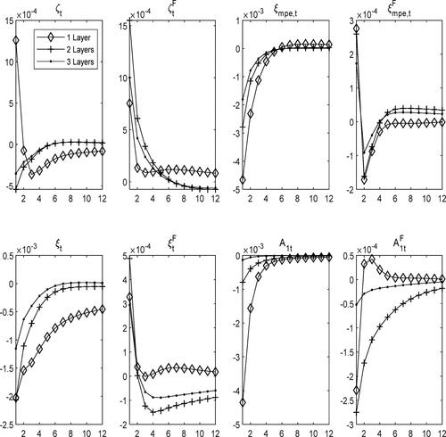
In order to verify the mechanism of multi-layer price stickiness, we make a counterfactual experiment here by considering an economy with 1–3 layer production chain, and compare the IRFs of different cases. In the same way, we compare the benchmark model with the one without shadow economy, in order to confirm its role on inflation smoothness.

Figure 4 compares IRFs with 1–3 production chain in the model settings, in which only one-layer production corresponds to the standard NK model. The figure shows that under the standard NK model, domestic consumption shock, monetary policy shock, investment shock and technology shock produce the largest impact of 0.13%, −0.48%, −0.12%, and −0.43% on CPI inflation, respectively. Under the model setting of two-layer production, domestic consumption shock, monetary policy shock, and technological shock cause CPI inflation change by −0.05%, −0.29%, and −0.09%, all lower than the result of the standard NK model with only one-layer production. As for domestic investment shock, although the highest impact in both cases is −0.2%, the two-layer results produce relatively lower IRF in the subsequent periods than the standard NK model. Finally, for the baseline model with three-layer production, the above four shocks make CPI inflation change by −0.48%, −0.28%, −0.2%, and −0.02% at most, much larger than the results of the above two cases. Moreover, the IRFs in three-layer production benchmark model show more inflation smoothness, which once again verifies the role of multi-layer price stickiness on inflation.

Figure 4. The smoothness effect of industrial structure on CPI inflation.

Source: Authors.

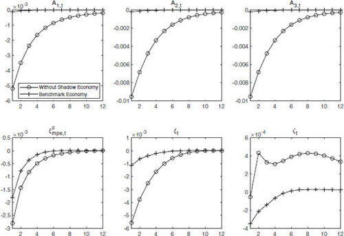
To verify the mechanism of shadow economy, we make another counterfactual simulation in the final product sector, which always has the largest proportions of informal production, and compares the IRFs of domestic shocks between the settings of the benchmark model and an economy in absence of shadow economy. Figure 5 shows that, compared with the benchmark model with shadow economy, in the latter case, the above four shocks cause a higher IRF under the model without shadow economy. This result is quite reasonable, since the shadow economy with a lower marginal cost makes the Philips curve flatter.

Figure 5. The smoothing effect of the shadow economy on inflation.

Source: Authors.

7. Conclusions

In summary, we establish a two-country DSGE model with a three-layer vertical industrial chain to study the dynamic characteristics of China's inflation. By introducing the vertical industrial chain, the multi-layer stickiness results in a smoothness effect of inflation. More importantly, inflation can not only be transmitted from top layer to bottom through cost channels, but also through mechanism of investment price effects and the intermediate products demand effects. In addition, considering that there is a large amount of informal economy in China, we introduce shadow economy in production to give a better explanation to China’s inflation dynamics.

We use quarterly data of China and the United States to calibrate and estimate the parameters. Variance decomposition and impulse response analysis also show that fluctuations in China's output and inflation are mainly caused by domestic shocks. Moreover, since the final goods production affects all types of price indices through its impact on investment prices, its technology shock constitutes the most important influencing factor in explaining all types of inflations.

Our policy implications are reflected in the following three aspects: First, the core conclusions show that with the deepening of the industrialization, the impact of exogenous shocks to macroeconomic variables such as output and inflation becomes smoother. This confirms that since the late 1980s, the world has maintained a low inflation rate for a long time, which helps to form ‘great stability’. At the same time, the conclusion also means that the future economic development of China's industrialization will decrease the volatility of macro economy, and the Chinese economy will become more stable in the future. Second, our conclusion also implies that domestic technology shock and monetary policy shock are the most important factors that cause inflation in China. In view of this, China’s future monetary policy should establish clear monetary policy rules, enhance the transparency of monetary policy implementation, reducing the impact of monetary policy shocks on inflation and output fluctuations. Finally, we cannot underestimate the impact of foreign shocks on China’s inflation, especially in the context of the current uncertain economic recovery in the United States, the impact of demand and monetary policy from the United States will have a non-negligible impact on China ’s inflation and other macroeconomic variables.

Disclosure statement

No potential conflict of interest was reported by the authors.

Notes

1 We adopt three levels instead of fewer or more vertical industrial structures mainly based on the following considerations. First, a single industrial structure cannot analyse the impact of external shocks on different industries, but the use of a two-level industrial structure, such as an upstream enterprise that produces intermediate products and a downstream enterprise that produces final products, is not enough to characterize difference between raw materials, processed industrial products and final consumer products in real world. Second, with an industrial structure of more than four levels, the model is more complex. Due to data limitations, it is difficult to calibrate and estimate a large number of parameters.

2 For symmetry of the model, the decision problem of country F is similar to that of country H, except for lack of shadow economy in each production layer. To save space, we put the content of country F in the appendix.

Appendix A

A.1 Households in country $F$

Similar to the setting of the household sector in country $H,$ households in country $F$ also obtain utility through consumption, currency holding and leisure. The utility function is given by (A.1) $$U^F=\sum _{t=0}^{\infty }{\beta }_{}^t{\varsigma }_t^F\left[\frac{{\left(C_t^F\right)}^{1-\sigma }}{1-\sigma }+\frac{{\left(M_t^F/P_{3,t}^F\right)}^{1-\psi }}{1-\psi }-\frac{{\left(L_t^F\right)}^{1+\upsilon }}{1+\upsilon }\right]$$(A.1)

Subject to the budget constraints (A.2) $$\begin{array}{c}{P}_{3,t}^F{C}_t^F+P_{I,t}^F{I}_t^F+M_t^F+\sum _{v_{t+1}}Q\left(v_{t+1}|v_t\right)B_{H,t+1}^F\left(v_{t+1}\right)/S_t\\ +\sum _{v_{t+1}}{Q}^F\left(v_{t+1}|v_t\right)B_{F,t+1}^F=W_t^F{L}_t^F+M_{t-1}^F+B_{H,t}^F\\ +B_{F,t}^F+T_t^F+P_{3,t}^F{\Theta }_t^F+R_{K,t}^F{K}_t^F\end{array}$$(A.2) where the consumption of households in country $F$ is also a composite of country $H$ and its domestic consumer goods, that is (A.3) $$C_t^F={\left[{\left(1-a_F\right)}^{1/\epsilon }{\left(C_{F,t}^F\right)}^{1-1/\epsilon }+a_F^{1/\epsilon }{\left(C_{H,t}^F\right)}^{1-1/\epsilon }\right]}^{\epsilon /\left(\epsilon -1\right)}$$(A.3)

Symmetrically, actual investment $I_t^F$ is composed of domestic investment products and imported investment products, that is (A.4) $$I_t^F={\left[{\left(1-a_I^F\right)}^{1/{\epsilon }_I}{\left(I_{F,t}^F\right)}^{1-1/{\epsilon }_I}+{\left(a_I^F\right)}^{1/{\epsilon }_I}{\left(I_{H,t}^F\right)}^{1-1/{\epsilon }_I}\right]}^{{\epsilon }_I/\left({\epsilon }_I-1\right)}$$(A.4)

Finally, the capital accumulation equation of the households in country $F$ is given by (A.5) $$K_{t+1}^F=\left(1-\delta \right)K_t^F+{\xi }_t^F\left[1-\Gamma \left(I_t^F/I_{t-1}^F\right)\right]I_t^F$$(A.5)

A.2 Production of primary products in country $F$

We set the production function of the primary product enterprises in country $F$ as (A.6) $$Y_{1,t}^F=A_{1,t}^F{\left(K_{1,t}^F\right)}^{{\alpha }_1}{\left(L_{1,t}^F\right)}^{1-{\alpha }_1}$$(A.6) where $A_{1,t}^F$ represents the technology level of primary goods production in country $F.$ $K_{1,t}^F$ and $L_{1,t}^F$ represent the amount of capital and labour input in primary goods production in country $F.$ We assume that the firm adopts the sticky pricing method of Calvo (1983), that is, the enterprises of country $F$ choose the optimal pricing ${\tilde{P}}_{1F,t}^F$ with probability $1-{\theta }_1^F$ in each period, and otherwise, the price remains unchanged. Since the production of country F only exists in the formal economy, we obtain the price dynamic equation of primary products: (A.7) $$\begin{array}{c}{\pi }_{1F,t}^F=\beta E_t{\pi }_{1F,t}^F+\frac{\left(1-{\theta }_1^F\right)\left(1-\beta {\theta }_1^F\right)}{{\theta }_1^F}\left[{\widehat{MC}}_{1,t}^F{}_{}+{\widehat{P}}_{3,t}^F-{\widehat{P}}_{1F,t}^F\right]\\ =\beta E_t{\pi }_{1F,t}^F+\frac{\left(1-{\theta }_1^F\right)\left(1-\beta {\theta }_1^F\right)}{{\theta }_1^F}\left[\left(1-{\alpha }_1\right){\widehat{w}}_t^F+{\alpha }_1{\widehat{r}}_{K,t}^F-{\widehat{A}}_{1,t}^F+{\widehat{P}}_{3,t}^F-{\widehat{P}}_{1F,t}^F\right]\end{array}$$(A.7)

A.3 Industrial goods production in country $F$

We assume that the production function of the industrial goods in country $F$ is: (A.8) $$Y_{2,t}^F=A_{2,t}^F{\left(Z_{1,t}^F\right)}^{{\chi }_1}{\left[{\left(K_{2,t}^F\right)}^{{\alpha }_2}{\left(L_{2,t}^F\right)}^{1-{\alpha }_2}\right]}^{1-{\chi }_1}$$(A.8) where $Z_{1,t}^F$ is the primary product used in the production of industrial goods in country $F,$ that is, $$Z_{1,t}^F={\left[{\left(1-{\kappa }_1^F\right)}^{1/{\phi }_1}{\left(Y_{1F,t}^F\right)}^{1-1/{\phi }_1}+{\left({\kappa }_1^F\right)}^{1/{\phi }_1}{\left(Y_{1F,t}^F\right)}^{1-1/{\phi }_1}\right]}^{{\phi }_1/\left({\phi }_1-1\right)}$$

$A_{2,t}^F$ represents the technology level of the production of primary products in country $F.$ $K_{2,t}^F$ and $L_{2,t}^F$ represent the amount of capital and labour input in the industrial goods production. Given the raw material purchase price index $P_{1,t}^F,$ wage $w_t,$ and return on capital of industrial products $r_{K,t}^F$ in country $F,$ the actual marginal cost of industrial products $M{C}_{2,t}^F$ in country $F$ is given by (A.9) $$M{C}_{2,t}^F=\frac{{\left[{\left(w_t^F\right)}^{1-{\alpha }_2}{\left(r_{K,t}^F\right)}^{{\alpha }_2}\right]}^{1-{\chi }_1}{\left(P_{1,t}^F/P_{3,t}^F\right)}^{{\chi }_1}}{A_{2,t}^F{\chi }_1^{{\chi }_1}{\left[\left(1-{\chi }_1\right){\alpha }_2^{{\alpha }_2}{\left(1-{\alpha }_2\right)}^{1-{\alpha }_2}\right]}^{1-{\chi }_1}}$$(A.9)

We make further assumption that the enterprises in country $F$ adopt the sticky pricing of Calvo (1983), that is, the enterprises choose the optimal pricing ${\tilde{P}}_{2H,t}^F$ with probability $1-{\theta }_2^F$ in each period, and otherwise the price remains unchanged. The price dynamic equation of industrial products can be obtained by (A.10) $${\pi }_{2F,t}^F=\beta E_t{\pi }_{2F,t+1}^F+\left(1-{\theta }_2^F\right)\left(1-\beta {\theta }_2^F\right)/{\theta }_2^F\left({\widehat{MC}}_{2,t}^F+{\widehat{P}}_{3,t}^F-{\widehat{P}}_{2F,t}^F\right)$$(A.10)

A.4 Final goods production in country $F$

We set the production function of the final goods in country $F$ as follows. (A.11) $$Y_{3,t}^F=A_{3,t}^F{\left(Z_{2,t}^F\right)}^{{\chi }_2}{\left[{\left(K_{3,t}^F\right)}^{{\alpha }_3}{\left(L_{3,t}^F\right)}^{1-{\alpha }_3}\right]}^{1-{\chi }_2}$$(A.11) Where $Z_{2,t}^F$ is the industrial product used in final goods production in country $F,$ that is, $Z_{2,t}^F={\left[{(1-{\kappa }_2^F)}^{1/{\phi }_2}{(Y_{2F,t}^F)}^{1-1/{\phi }_2}+{({\kappa }_2^F)}^{1/{\phi }_2}{(Y_{2F,t}^F)}^{1-1/{\phi }_2}\right]}^{{\phi }_2/({\phi }_2-1)}.$ $A_{3,t}^F$ represents the technology level of the production in country $F.$ $K_{2,t}^F$ and $L_{2,t}^F$ represent the amount of capital and labour input in the production. Given the industrial products purchase price index $P_{2,t}^F,$ wage $w_t{}^F,$ and return on capital of industrial products $r_{K,t}^F$ in country $F,$ the actual marginal cost of final products $M{C}_{3,t}^F$ in country $F$ is given by (A.12) $$M{C}_{3,t}^F=\frac{{\left[{\left(w_t^F\right)}^{1-{\alpha }_3}{\left(r_{K,t}^F\right)}^{{\alpha }_3}\right]}^{1-{\chi }_2}{\left(P_{2,t}^F/P_{3,t}^F\right)}^{{\chi }_2}}{A_{3,t}^F{\chi }_2^{{\chi }_2}{\left[\left(1-{\chi }_2\right){\alpha }_3^{{\alpha }_3}{\left(1-{\alpha }_3\right)}^{1-{\alpha }_3}\right]}^{1-{\chi }_2}}$$(A.12)

Since entrepreneurs adopt the sticky pricing of Calvo (1983), the price dynamic equation of the final product is (A.13) $${\pi }_{3F,t}^F=\beta E_t{\pi }_{3F,t+1}^F+\frac{\left(1-{\theta }_3^F\right)\left(1-\beta {\theta }_3^F\right)}{{\theta }_3^F}\left({\widehat{MC}}_{3,t}^F+{\widehat{P}}_{3,t}^F-{\widehat{P}}_{3F,t}^F\right)$$(A.13)

A.5 Market equilibrium

The equilibrium of our model includes product market equilibrium, labour market equilibrium, capital market equilibrium and bond market equilibrium. The equilibrium condition of the product market is given by (A.14) $$Y_{1,t}=Y_{1H,t}+Y_{1H,t}^F$$(A.14) (A.15) $$Y_{1,t}^F=Y_{1F,t}+Y_{1F,t}^F$$(A.15) (A.16) $$Y_{2,t}=Y_{2H,t}+Y_{2H,t}^F$$(A.16) (A.17) $$Y_{2,t}^F=Y_{2F,t}+Y_{2F,t}^F$$(A.17) (A.18) $$\begin{array}{c}{Y}_{3,t}=C_{3H,t}+C_{3H,t}^F+I_{H,t}+I_{H,t}^F\\ =\left(1-a_H\right){\left(\frac{P_{3H,t}}{P_{3,t}}\right)}^{-\epsilon }{C}_t+a_F{\left(\frac{P_{3H,t}^F}{P_{3,t}^F}\right)}^{-\epsilon }{C}_t^F\\ +\left(1-a_I\right){\left(\frac{P_{3H,t}}{P_{I,t}}\right)}^{-{\epsilon }_I}{I}_t+a_I^F{\left(\frac{P_{3H,t}^F}{P_{I,t}^F}\right)}^{-{\epsilon }_I}{I}_t^F\end{array}$$(A.18) (A.19) $$\begin{array}{c}{Y}_{3,t}^F=C_{3F,t}+C_{3F,t}^F+I_{F,t}+I_{F,t}^F\\ =a_H{\left(\frac{P_{3F,t}}{P_{3,t}}\right)}^{-\epsilon }{C}_t+\left(1-a_F\right){\left(\frac{P_{3F,t}^F}{P_{3,t}^F}\right)}^{-\epsilon }{C}_t^F\\ +a_I^{}{\left(\frac{P_{3F,t}}{P_{I,t}}\right)}^{-{\epsilon }_I}{I}_t+\left(1-a_I^F\right){\left(\frac{P_{3F,t}^F}{P_{I,t}^F}\right)}^{-{\epsilon }_I}{I}_t^F\end{array}$$(A.19)

The conditions for labour market equilibrium are (A.20) $$L_t=L_{1,t}+L_{2,t}+L_{3,t}$$(A.20) (A.21) $$L=L_{1t}^F+L_{2t}^F+L_{3t}^F$$(A.21)

The equilibrium conditions of the capital market are (A.22) $$K_t=K_{1,t}+K_{2,t}+K_{3,t}$$(A.22) (A.23) $$K=K_{1t}^F+K_{2t}^F+K_{3t}^F$$(A.23)

The equilibrium conditions of the bond market are (A.24) $$B_{H,t}+B_{H,t}^F=0$$(A.24) (A.25) $$B_{F,t}+B_{F,t}^F=0$$(A.25)

References

- Bouakez, H., Rachedi, O., & Santoro, E. (2022). The government spending multiplier in a multi-sector economy. American Economic Journal: Macroeconomics (Accepted). https://www.aeaweb.org/articles?id=10.1257/mac.20200213
- Calvo, G. A. (1983). Staggered prices in a utility-maximizing framework. Journal of Monetary Economics, 12(3), 383–398. https://doi.org/10.1016/0304-3932(83)90060-0
- Carvalho, C., Lee, J. W., & Park, W. Y. (2021). Sectoral price facts in a sticky-price model. American Economic Journal: Macroeconomics, 13(1), 216–256. https://doi.org/10.1257/mac.20190205
- Chow, G., & Wang, P. (2010). The empirics of inflation in China. Economics Letters, 109(1), 28–30. https://doi.org/10.1016/j.econlet.2010.07.009
- Christiano, L. J., Eichenbaum, M., & Evans, C. L. (2005). Nominal rigidities and the dynamic effects of a shock to monetary policy. Journal of Political Economy, 113(1), 1: 1–45. https://doi.org/10.1086/426038
- Clarida, R., Gali, J., & Gertler, M. (1999). The science of monetary policy: a new Keynesian perspective. No. w7147. National Bureau of Economic Research.
- Colombo, E., Onnis, L., & Tirelli, P. (2016). Shadow Economies at Times of Banking Crises: Empirics and Theory. Journal of Banking & Finance (vol. 62(C), pp. 180–190). Elsevier.
- Devereux, M. B., Lane, P. R., & Juanyi, X. (2006). Exchange rates and monetary policy in emerging market economies. The Economic Journal, 116(511), 478–506. https://doi.org/10.1111/j.1468-0297.2006.01089.x
- Funke, M., Mehrotra, A., & Yu, H. (2015). Tracking Chinese CPI inflation in real time. Empirical Economics, 48(4), 1619–1641. https://doi.org/10.1007/s00181-014-0837-3
- Gali, J., & Gertler, M. (1999). Inflation dynamics: A structural econometric analysis. Journal of Monetary Economics, 44, 195–222.
- He, Q., Liu, F., & Qian, Z. (2017). Housing prices and business cycle in China: A DSGE analysis. International Review of Economics & Finance (vol. 52(C), pp. 246–256). Elsevier.
- Horvath, M. (2000). Sectoral shocks and aggregate fluctuations. Journal of Monetary Economics, 45(1):69–106.
- Huang, K. X., & Liu, Z. (2001). Production chains and general equilibrium aggregate dynamics. Journal of Monetary Economics, 48(2), 437–462. https://doi.org/10.1016/S0304-3932(01)00078-2
- Huang, K. X., & Liu, Z. (2007). Business cycles with staggered prices and international trade in intermediate inputs. Journal of Monetary Economics, 54(4), 1271–1289. https://doi.org/10.1016/j.jmoneco.2006.05.016
- Kim, K. & Kim Y. (2006). How important is the intermediate input channel in explaining sectoral employment comovement over the business cycle?. Review of Economic Dynamics, 9, 659–682.
- Li, D., Minford, P., & Peng, Z. (2015). A DSGE model of China. Applied Economics, Taylor & Francis Journals, 47(59), 6438–6460.
- Moro, A. (2012). The structural transformation between manufacturing and services and the decline in the U.S. GDP volatility. Review of Economic Dynamics, 15(3), 402–415. https://doi.org/10.1016/j.red.2011.09.005
- Pinto, J. (2021). Production network structure, service share, and aggregate volatility. Review of Economic Dynamics, 39, 146–173.
- Rabanal, P. (2007). Does inflation increase after a monetary policy tightening? Answers based on an estimated DSGE model. Journal of Economic Dynamics and Control, 31(3), 906–937. https://doi.org/10.1016/j.jedc.2006.01.008
- Rudd, J. B., Whelan, K, & Board of Governors of the Federal Reserve System (2005). Modelling inflation dynamics: A critical review of recent research. Finance and Economics Discussion Series, 2005(66), 1–53. https://doi.org/10.17016/FEDS.2005.66
- Rudd, J., & Whelan, K. (2006). Can rational expectations sticky-price models explain inflation dynamics? American Economic Review, 96(1), 303–320. https://doi.org/10.1257/000282806776157560
- Smets, F., & Wouters, R. (2003). An estimated dynamic stochastic general equilibrium model of the Euro area. Journal of the European Economic Association, 1(5), 1123–1175. https://doi.org/10.1162/154247603770383415
- Solis-Garcia, M., & Xie, Y. (2018). Measuring the size of the shadow economy using a dynamic general equilibrium model with trends. Journal of Macroeconomics, 56(C), 258–275. https://doi.org/10.1016/j.jmacro.2018.04.004
- Wong, C. Y., & Eng, Y. K. (2010). Vertically globalized production structure in New Keynesian Phillips curve. The North American Journal of Economics and Finance, 21(2), 198–216. https://doi.org/10.1016/j.najef.2009.03.004
Appendix A
A.1 Households in country